Quantitative Soundscape Analysis to Understand Multidimensional Features - Frontiers
←
→
Page content transcription
If your browser does not render page correctly, please read the page content below
ORIGINAL RESEARCH
                                                                                                                                          published: 05 August 2021
                                                                                                                                    doi: 10.3389/fmars.2021.672336

                                            Quantitative Soundscape Analysis to
                                            Understand Multidimensional
                                            Features
                                            Dylan Charles Wilford 1,2,3* , Jennifer L. Miksis-Olds 2 , S. Bruce Martin 4 ,
                                            Daniel R. Howard 2,5 , Kim Lowell 3 , Anthony P. Lyons 2,3 and Michael James Smith 3
                                            1
                                              School of Marine Science and Ocean Engineering, University of New Hampshire, Durham, NH, United States, 2 Center
                                            for Acoustics Research and Education, Institute for the Study of Earth, Oceans, and Space, University of New Hampshire,
                                            Durham, NH, United States, 3 Center for Coastal and Ocean Mapping, University of New Hampshire, Durham, CA,
                                            United States, 4 JASCO Applied Sciences (Canada) Ltd., Victoria, BC, Canada, 5 Department of Biological Sciences, College
                                            of Life Sciences and Agriculture, University of New Hampshire, Durham, NH, United States

                                            A methodology for the analysis of soundscapes was developed in an attempt to
                                            facilitate efficient and accurate soundscape comparisons across time and space. The
                                            methodology consists of a collection of traditional soundscape metrics, statistical
                                            measures, and acoustic indices that were selected to quantify several salient properties
                                            of marine soundscapes: amplitude, impulsiveness, periodicity, and uniformity. The
                         Edited by:
                                            metrics were calculated over approximately 30 h of semi-continuous passive acoustic
                        Ana Sirovic,
  Texas A&M University at Galveston,        data gathered in seven unique acoustic environments. The resultant metric values
                      United States         were compared to a priori descriptions and cross-examined statistically to determine
                       Reviewed by:         which combination most effectively captured the characteristics of the representative
               Craig Aaron Radford,
          The University of Auckland,       soundscapes. The best measures of amplitude, impulsiveness, periodicity, and
                         New Zealand        uniformity were determined to be SPLrms and SPLpk for amplitude, kurtosis for
                 Megan F. McKenna,
                                            impulsiveness, an autocorrelation based metric for periodicity, and the Dissimilarity index
    Stanford University, United States
                                            for uniformity. The metrics were combined to form the proposed “Soundscape Code,”
               *Correspondence:
              Dylan Charles Wilford         which allows for rapid multidimensional and direct comparisons of salient soundscape
         dcw1017@wildcats.unh.edu           properties across time and space. This initial characterization will aid in directing further
                   Specialty section:
                                            analyses and guiding subsequent assessments to understand soundscape dynamics.
         This article was submitted to
                                            Keywords: soundscape, kurtosis, Dissimilarity Index, ocean sound, metrics, marine acoustics
                   Ocean Observation,
               a section of the journal
          Frontiers in Marine Science
                                            INTRODUCTION
        Received: 25 February 2021
           Accepted: 25 June 2021           Ocean sound conveys a wealth of information due to the highly efficient manner in which
         Published: 05 August 2021
                                            acoustic energy travels through the water. Studying ambient ocean sound provides information
                             Citation:      on vocalizing marine life, ocean dynamics, and human use of the ocean (Hildebrand,
         Wilford DC, Miksis-Olds JL,        2009; Pijanowski et al., 2011; Howe et al., 2019). In recognition of its inherent value,
   Martin SB, Howard DR, Lowell K,
                                            ocean sound has been recently accepted as an Essential Ocean Variable (EOV) by the
      Lyons AP and Smith MJ (2021)
   Quantitative Soundscape Analysis
                                            Global Ocean Observing System (GOOS) Biology and Ecosystem Panel (Ocean Sound EOV,
     to Understand Multidimensional         2018). EOVs are approved based on three considerations: (1) relevance in helping solve
 Features. Front. Mar. Sci. 8:672336.       scientific questions and addressing societal needs, (2) contributions to improving marine
   doi: 10.3389/fmars.2021.672336           resource management, and (3) feasibility for global observation regarding cost effectiveness,

Frontiers in Marine Science | www.frontiersin.org                                 1                                          August 2021 | Volume 8 | Article 672336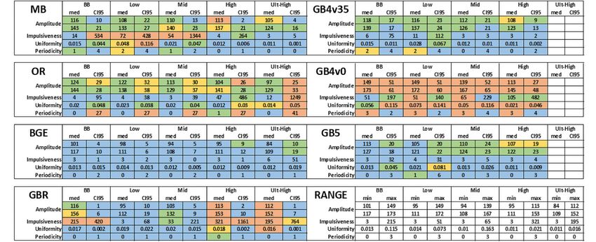
Wilford et al.                                                                                                      Quantitative Soundscape Analysis

technology, and human capabilities1 . In the context of ocean               averaging have yielded differences in final metric results of over
sound, inclusion in the GOOS framework provides a formal                    10 dB in previous works (Merchant et al., 2012; Hawkins et al.,
structure for recording ocean sound. Implementation of the                  2014). Some methodology descriptions are so vague it is nearly
ocean sound EOV will help to guide scientific data collection to            impossible to determine averaging times, integration windows,
ensure consistency and appropriate comparisons in soundscape                and exactly which metric is being calculated (McKenna et al.,
analysis and ocean sound studies.                                           2016). To accurately report important soundscape information,
    A soundscape is an acoustic environment tied to the                     efforts must be made to standardize the way in which researchers
function of a given landscape or marine habitat, and it is                  acquire, process, analyze, and report acoustic metrics.
the sum of all sounds present; ISO 18405 defines soundscape                     Many analysis methods produce graphical outputs, which
as the characterization of the ambient sound in terms of its                are assessed visually but can become cumbersome when
spatial, temporal, frequency attributes, and the types of sources           many comparisons need to be quantitative across time or
contributing to the sound field. Defining and characterizing                space. Graphical information, supplemented with standardized
the soundscape is an important step in the task of assessing,               quantitative analysis of the multidimensional soundscape within
monitoring, and comparing global acoustic environments. By                  an accepted framework would produce thorough, accurate, and
utilizing soundscape analysis and ocean sound, researchers                  easily comparable results for acoustic recordings. A method
can better understand ocean dynamics (Radford et al., 2010;                 that resembles this type of standardized quantitative analysis
McWilliam and Hawkins, 2013; Miksis-Olds et al., 2013;                      was adopted by The World Meteorology Organization (WMO)
Staaterman et al., 2014), biodiversity and ecosystem health (Parks          for comparing and reporting the state of sea ice that
et al., 2014; Staaterman et al., 2014), and the risk of anthropogenic       encompasses multidimensional information: ice coverage, stage
impacts on marine life (Weilgart, 2007; Carroll et al., 2017).              of development, age, thickness and form. The WMO system
    Traditionally, sound is analyzed by measuring the sound                 for reporting sea ice is commonly referred to as the “egg code”
pressure level (Sound Pressure Level; SPL), and other source-               (JCOMM Expert Team on Sea Ice, 2014). This egg code presents
and amplitude-related parameters such as the number of sources              standard ice characteristics in a clear and succinct manner, and
detected, source classification, localization of detectable sources,        the multidimensional nature of the egg code reports a variety
or sound exposure level (SEL) (Martin et al., 2019). Recently,              of relevant ice properties; “one size fits all” measures are rarely
researchers have developed and applied metrics mathematically               adequate in describing dynamic environments (Figure 1). The
summarizing acoustic properties and comparing them with                     idea of a “measure” like the egg code that captures and reports
independent ecological data to understand the types of sources              salient information about an environment is the inspiration
present in a soundscape. For example, the Acoustic Complexity               for the proposed soundscape code. While the egg code reports
Index (ACI) was proposed as a proxy for biodiversity Sueur                  multiple dimensions of the environmental “feature” ice, the
et al. (2008), and (Pieretti et al., 2011) demonstrated the                 proposed soundscape code reports multiple dimensions of the
efficacy of the Entropy Index (H-index) and the Dissimilarity               environmental “feature,” sound pressure.
Index (D-index) at highlighting biodiversity of a terrestrial                   Amplitude, periodicity, impulsiveness, and uniformity
environment. Application of acoustic biodiversity indices in a              are physical soundscape properties that are important to
marine environment have yielded mixed results (Parks et al.,                understanding soundscapes and the distribution of sound energy
2014; Staaterman et al., 2017; Bohnenstiehl et al., 2018; Bolgan            across time, space, and frequency (Table 1). The objective of
et al., 2018). Further investigation into the utility of acoustic           this study was to identify the optimal suite of metrics across
indices in marine applications is needed to assess their efficacy.          the general soundscape properties (amplitude, impulsiveness,
    Even though ocean ambient sound and soundscape research                 periodicity, and uniformity) to create a soundscape code
has been conducted for decades, the ocean community has still               infrastructure for comparing soundscapes. Multiple metrics
not reached a consensus on the optimal way to accurately report             within each soundscape property (Table 2) were selected and
and compare important aspects of ocean sound. Ocean sound                   applied to a diverse set of soundscapes to identify the metric
studies are not trivial endeavors, and the complexity of ocean              that best captured the salient aspects of the acoustic recordings.
sound dynamics, combined with a lack of formal standards,                   Comparing the acoustic properties of soundscapes is not meant
guidelines, and consistent methods, make soundscape analyses                to be an exhaustive assessment, but rather an initial analysis to
and meaningful comparisons difficult. The methodologies                     understand some of the dynamics of acoustic environments and
utilized by researchers are often tailored to a specific study,             guide subsequent analysis for more targeted assessments. The
which focuses on answering the question at hand, but contributes            resulting product forms the proposed soundscape code, which
little to the understanding of soundscape dynamics on a                     provides a framework for comparing soundscape properties
large regional or global scale if the results cannot be easily              across space and time utilizing metrics that capture spectral and
interpreted or compared to data from other areas. Studies often             temporal properties of acoustic environments; characterizing
fail to clearly report metric input parameters critical to the              acoustic environments in terms of spatial, spectral, and temporal
determination of the final metric value; ambiguities in reporting           acoustic properties directly relates to the ISO 18405 definition
can make replicating study methodologies difficult, and can lead            of a soundscape.
to erroneous comparisons. For example, different methods of                     Sound level statistics and measures of the amplitude of
                                                                            acoustic power and energy are used frequently in ocean sound
1
    https://goosocean.org/index                                             studies. The root-mean-square (rms) SPL captures the average

Frontiers in Marine Science | www.frontiersin.org                       2                                     August 2021 | Volume 8 | Article 672336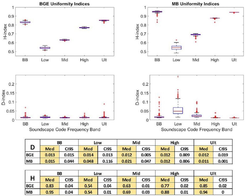
Wilford et al.                                                                                                               Quantitative Soundscape Analysis

  FIGURE 1 | WMO egg code (JCOMM Expert Team on Sea Ice, 2014). Contained in the simple oval are data regarding concentrations, stages of development, and
  form of ice. Code conforms to an international convention.

sound pressure amplitude of the corresponding environment                        Lobel, 1992), and the rhythmic rasping of the California spiny
(SPLrms ). Though susceptible to upward bias from loud,                          lobster (Patek et al., 2009) are examples of real world ocean
intermittent sounds, SPLrms is the most ubiquitous acoustic                      signals that are periodic. The proposed soundscape code focuses
metric (Merchant et al., 2015). SPLrms does not capture all                      on periodicities that (1) impose physical characteristics to a
the important amplitude information of a soundscape such                         soundscape over short time periods, (2) occur on time scales of
as maximum sound pressure levels (SPLpk ), the sound floor                       less than a minute, and (3) can be captured by metrics calculated
(quietest periods in a soundscape), or sound exposure level.                     over a single minute of acoustic data. A metric for capturing
Reporting both the SPLrms and SPLpk provides detail on average                   larger scale periodicity related to diel, season, or annual cycles
sound amplitude as well as information on the range of                           was not explored in this project but could be assessed using a
sound amplitude.                                                                 time series of the individual soundscape code parameters. To
    Impulsive sounds are defined qualitatively as sounds that are                our knowledge no metric designed specifically for quantifying
of short duration, have rapid rise times, and high sound levels                  the content of periodic signals in an acoustic environment exists,
(NIOSH, 1998; NMFS, 2018). A wide variety of sound sources                       so metrics from other fields were repurposed as candidates
produce pulsed acoustic signatures which means that it is possible               to represent the periodicity property in the soundscape code.
for the impulsiveness of a soundscape to be used as an indication                Cepstrum was first proposed as a tool for analyzing periodic
of source presence/absence. Impulsive sounds can potentially                     seismological data (Bogert et al., 1963), where the arrival of
have physiological impacts on fish (Halvorsen et al., 2012a,b;                   various waves and phases could be considered as distorted echoes.
Casper et al., 2013a,b), and marine mammals (Lucke et al., 2009;                 Cepstrum is not widely used in marine soundscape studies, but
Kastelein et al., 2015; Southall et al., 2019), so it is also a valuable         has been used with efficacy in a variety of mechanical analyses,
property to consider from a regulatory perspective as well as a                  and it is considered underutilized by those that use it (Randall,
physical characteristic. Regulations lack quantitative definitions               2017). Time lagged autocorrelation has been used to characterize
regarding the difference between impulsive and non-impulsive                     soundscapes in terms of the dominant source types (Martin et al.,
sounds, but several metrics for quantifying impulsiveness have                   2019), and was repurposed in this study to quantify the content
been suggested including kurtosis, crest factor and Harris impulse               of periodic signals detected in a soundscape.
factor (Erdreich, 1986; Starck and Pekkarinen, 1987; Kastelein                       Soundscape uniformity is the degree to which the signals
et al., 2017). All three were initially considered candidate metrics             change over time in terms of temporal and frequency attributes
to represent impulsiveness in the soundscape code, but Harris                    of the soundscape. It answers the question “to what degree are the
impulse factor was removed from consideration due to constraint                  sounds similar or different?” and describes the dynamic nature of
in the range of the metric and the resulting implications for future             a given soundscape. The inclusion of the uniformity property in
use in comparative analysis.                                                     the soundscape code was motivated by the widespread interest
    The term periodicity is inherently general; periodicity can                  in biodiversity, and the use of passive acoustic monitoring
refer to a pattern that repeats over the course of a year,                       techniques to study biodiversity remotely (Peet, 1974; Pimm and
month, day, hour, or second. Seismic airgun signals (Greene                      Lawton, 1998; Sueur et al., 2014). A suite of quantitative indices
and Richardson, 1988), echolocation clicks (Clarke et al.,                       has been developed and geared toward quantifying different
2019), pulsed fish or whale vocalizations (Watkins et al., 1987;                 properties of acoustic environments: Acoustic Complexity Index

Frontiers in Marine Science | www.frontiersin.org                            3                                         August 2021 | Volume 8 | Article 672336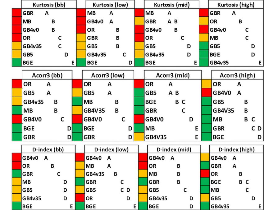
Wilford et al.                                                                                                                    Quantitative Soundscape Analysis

TABLE 1 | Literature selected to emphasize how authors implement a variety of acoustic metrics.

Topic                                                        Metrics                                          Soundscape code              References
                                                                                                              Property

Comparison of reef sound signatures–spatial                  Max/min sound intensity and corresponding        Amplitude                    Bertucci et al., 2015
comparison                                                   frequency (day, dusk, dawn)
                                                             Mean sound intensity (linear mean)

Comparison of reef sound signatures–spatial                  PSD (smoothed)                                   Amplitude                    Radford et al., 2014
comparison                                                   Mean sound intensity (dB mean)

Soundscape of the shallow waters of a Mediterranean          Monthly median root-mean-square level of the     Amplitude                    Buscaino et al., 2016
marine protected area–temporal comparison                    sound pressure (SPLrms) (per octave band/bb)     Uniformity
                                                             Day/night median SPLrms (per octave band/bb)     Impulsiveness
                                                             Day/night median PSD
                                                             Filtered Acoustic Complexity Index (ACI;
                                                             removal of snapping shrimp sounds)

A comparison of inshore marine soundscapes–spatial           ACI                                              Amplitude Uniformity         McWilliam and
comparison                                                   Acoustic Diversity Index (ADI)                                                Hawkins, 2013
                                                             PSD

The not so silent world: measuring arctic, equatorial,       Daily median sound levels                        Amplitude                    Haver et al., 2017
and Antarctic soundscapes in the Atlantic                    Long term spectral averages (LTSA)
ocean–spatial comparison

Evaluating changes in the marine soundscape of an            3–5 month spectrograms                           Amplitude                    Lin et al., 2019
offshore wind farm–temporal comparison                       Median/mean PSD

Soundscapes from a tropical Eastern Pacific reef and         Mean PSD over recording period plotted in        Amplitude Periodicity        Staaterman et al., 2013
Caribbean sea reef–spatial comparison                        100Hz bins and color mapped

Localized coastal habitats have distinct underwater          Sound intensity over 4 freq bands: 100–800 Hz,   Amplitude                    Radford et al., 2010
sound signatures–spatial comparison                          800 Hz–2.5 kHz, 2.5–20 kHz, 20 k–24 kHz
                                                             Proportion of sound intensity (per frequency
                                                             bands outlined previously)
                                                             Dusk/noon PSD

Assessing marine ecosystem acoustic diversity across         H-index                                          Uniformity                   Parks et al., 2014
ocean basins–spatial comparison

Marine soundscape as an additional biodiversity              ACI                                              Amplitude                    Pieretti et al., 2017
monitoring tool: a case study from the Adriatic Sea          PSD                                              Uniformity
                                                                                                              Periodicity

Investigating the utility of ecoacoustic metrics in marine   ACI                                              Impulsiveness                Bohnenstiehl et al.,
soundscapes                                                  H-index                                                                       2018

Basin-Wide contributions to the underwater                   1/3 octave levels                                Impulsiveness                Kyhn et al., 2019
soundscape by multiple seismic surveys with                  Mean instantaneous pressure level
implications for marine mammals in Baffin bay                Sound exposure level (SEL)

Increases in deep ocean ambient noise in the NE              Spectral averages                                Amplitude                    McDonald et al., 2006
pacific–temporal comparison

(ACI), H-index, D-index, and Acoustic Richness (AR). These                             mixed results (Parks et al., 2014; Harris et al., 2016). Harris
indices have been widely used in terrestrial acoustic studies to                       et al. (2016) found that H values exhibited a dependence on
measure biodiversity and species richness (Sueur et al., 2008,                         the size of the fast Fourier transform (FFT) window, and at a
2014; Pieretti et al., 2011, 2017). For the D-index, Sueur et al.                      window length of 512 showed little correlation to typical diversity
(2008) utilized a measure that estimated the compositional                             measures, but correlation increased with spectral resolution.
dissimilarity between two communities. Within this work, the                           Parks et al. (2014) had to remove noise from a seismic survey
D-index is applied to two consecutive acoustic recordings in                           before finding a significant connection between the H index
an effort to capture the acoustic differences and measure the                          and sampled biodiversity. Because H-index was designed to
acoustic uniformity. The Entropy Index (H) has been used                               increase with signal diversity in time and frequency, it was
as a proxy for biodiversity in the marine environment with                             repurposed in this study to represent acoustic uniformity, which

Frontiers in Marine Science | www.frontiersin.org                                  4                                        August 2021 | Volume 8 | Article 672336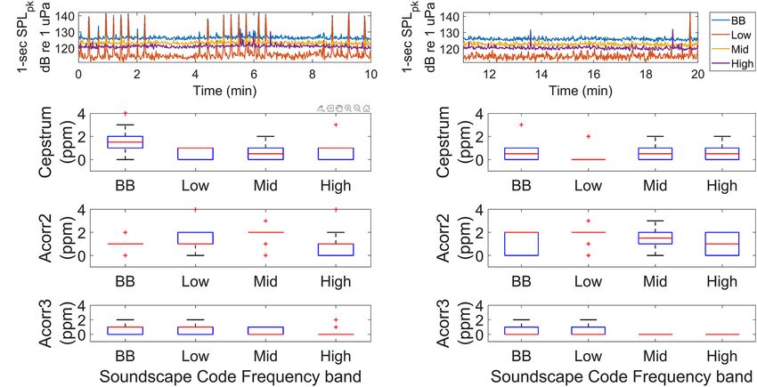
Wilford et al. Quantitative Soundscape Analysis
TABLE 2 | Soundscape properties and corresponding metrics, statistical measures, and indices investigated for inclusion in the soundscape code.
Soundscape Property Description Quantifying Measure
Amplitude Can be conceptualized as the “loudness” of an environment. Describes the effective SPLrms, SPLpk
sound level across time.
Impulsiveness Impulses are characterized as being broadband with rapid rise times, short durations, Kurtosis, Crest Factor
and high peak sound pressures. Impulsiveness of a soundscape would describe the
presence and magnitude of signals that can be characterized as impulsive.
Periodicity Describes the repetitive nature of sounds in the soundscape. The timescale of the Time lagged autocorrelation,
periodic activity is an important factor here; pulsed signals with short Cepstrum
inter-pulse-intervals like seismic surveys, pile driving, and pulsed minke whale
vocalizations are periodic; repeating acoustic events like dawn or evening chorus are
also periodic, but on much larger time scales.
Uniformity Describes the diversity of a system. In an acoustic context: to what degree are all the H-index, D-index
sounds similar or different across time?
shares similarities with the principle of acoustic diversity that the and above (broadband; BB). These frequency bands were
metric was built on. chosen because the dominant frequencies of many signals can
be isolated into a single soundscape code frequency band.
Data from Biogully East (BGE) was low pass filtered with
MATERIALS AND METHODS a passband out to 32 kHz to provide a uniform analysis
in the Ultra-High band across Melville Bay (MB), Great
The datasets used to assess the performance of the candidate Barrier Reef (GBR), Orsted (OR), and BGE. Sample rate
metrics for use in the soundscape code were selected from a restrictions precluded analysis of the Ultra-High band at the
pool of passive acoustic data that had already been analyzed, Grand Banks sites (GB4v0, GB4v35, and GB5). The high band
and in some cases, used in publications (Martin et al., 2017, at GB5 was included, even though the data could only be
2019, 2020; Martin and Barclay, 2019). Soundscape code resolved up to 8 kHz due to the sample rate at this site
datasets were picked based on previous knowledge of activity (16 kHz) (Table 2).
in the soundscape region. Digital passive acoustic data were The metrics assessed for the soundscape code were calculated
converted to pressure data, and then metrics were calculated over one-min time windows. The one-min time window is a
over each pressure time series. The metrics were analyzed standard time length in soundscape analysis and corresponds
to determine the optimal combination for capturing salient with the human auditory experience (Ainslie et al., 2018).
quantitative aspects of a soundscape. Each dataset was collected All FFTs performed in calculating soundscape code metrics
using Autonomous Multi-channel Acoustic Recorders (AMAR, used 1-second time windows. The median and 95% confidence
JASCO Applied Sciences) that sampled at a variety of sample interval of each metric was reported for each site and analyzed.
rates and durations (Table 3). Recorders were deployed Acorr2, acorr3, SPLrms , SPLpk , kurtosis, crest factor, D-index, and
intermittently between 2012 and 2016 at the seven different H-index were calculated using custom code written in MATLAB
locations. While the sites may not all be unique in their (2019); The Mathworks Inc., Natick, MA, United States.
location, the acoustic content of their recordings was unique; Sound pressure level (SPL), reported in logarithmic decibel
GB5 is actually about 70 km from GB4v35 and GB4v0, and (dB) units relative to a reference pressure of 1 µPa, is the
while the latter two share the same site location designation, most common amplitude metric reported in ocean sound studies
the datasets were recorded weeks apart. The seven data sets (Equation 1)
contain a variety of human-generated, natural biologic, and s Z
natural abiotic sounds including sounds from a seismic survey,
!
1 T p2 (t)
impact pile driving, vessel passages, ice calving and icebergs, fin SPLrms = 20log10 dt (1)
T 0 p2ref
(Balaenoptera physalus) and humpback whale (Megaptera
novaeangliae) vocalizations, northern bottlenose whale where Pref is reference pressure, p(t) is the instantaneous pressure
(Hyperoodon ampullatus) and common dolphin (Delphinus at time (t), and T is the analysis window duration (Madsen,
delphis) whistles and echolocation, and shallow-water reef 2005; Thompson et al., 2013; Merchant et al., 2015). The SPLpk
sounds including foraging urchins, snapping shrimp, and fish has added value as an amplitude metric, as it is also a relevant
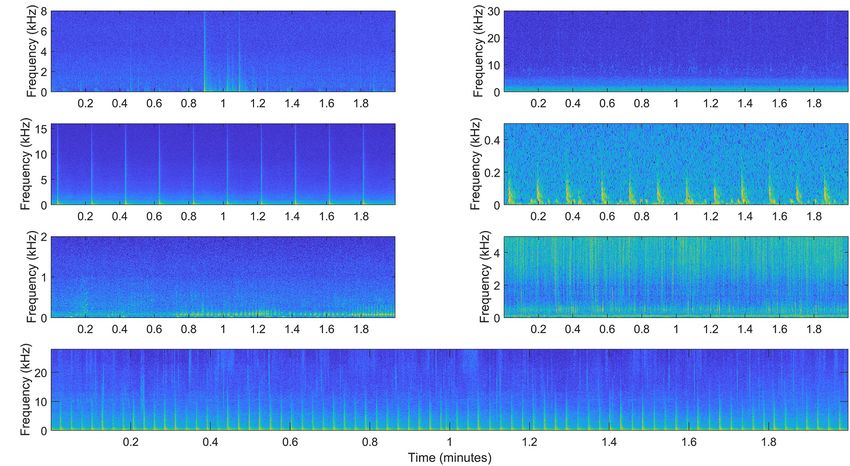
grunts (Figure 2). The biological sounds present in the data measure in determining the risk of physical damage in auditory
sets are representative of the diversity of marine life and sounds systems (Coles et al., 1968) (Equation 2).
produced ocean wide. !
p2max (t)
Data Processing SPLpk = 10log10 (2)
p2ref
Five frequency bands were selected for soundscape code analysis:
(1) 10–100 Hz (Low), (2) 100–1,000 Hz (Mid), (3) 1–10 kHz Because the SPLpk and SPLrms metrics were identified from
(High), (4) 10 kHz and above (Ultra-High), and (5) 10 Hz previously published work as well-established and effective
Frontiers in Marine Science | www.frontiersin.org 5 August 2021 | Volume 8 | Article 672336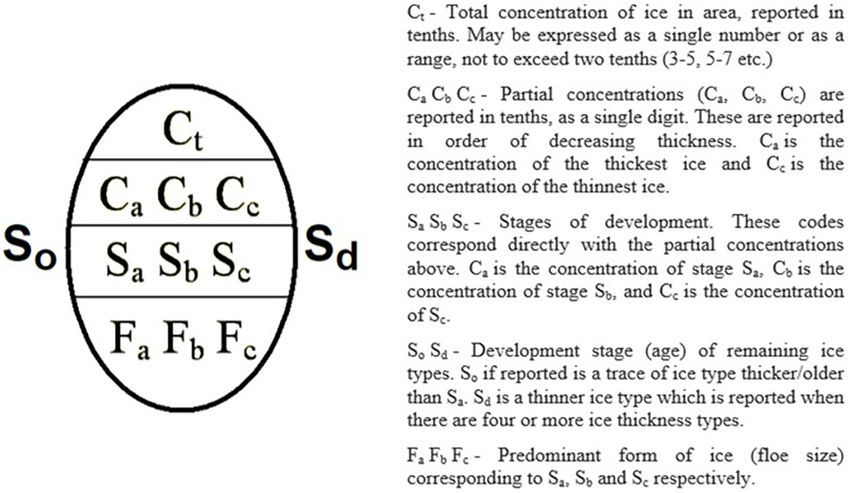
Wilford et al.                                                                                                                             Quantitative Soundscape Analysis

TABLE 3 | Soundscape code dataset descriptions and data collection parameters.

Data set (Site              Location                    Ecosystem            Latitude        Longitude      Depth           Sample                Duration     Duty cycle
abbreviation)                                           Type                 (◦ North)        (◦ East)     (meters)        Rate (kHz)              (min)         (min)

Melville Bay (MB)           Baffin Bay (Greenland)      Arctic                  75.3           −58.6         370                     64             240         continuous
Biogully East (BGE)         Nova Scotian Shelf          Open Ocean              43.8           −58.9        2000                    250             250         continuous
                                                        (deep)
Grand Banks (GB4v0)         Nova Scotian Shelf          Open Ocean              45.4           −48.8         112                     32             204         continuous
Grand Banks (GB4v35)        Nova Scotian Shelf          Open Ocean              45.4           −48.8         112                     32             354         continuous
Grand Banks (GB5)           Nova Scotian Shelf          Open Ocean              44.9           −49.3         119                     16             360         continuous
Great Barrier Reef          Wheeler Reef (Great         Tropical Reef          −18.8           147.5            18                   64             112            7/14
(GBR)                       Barrier Reef)               (shallow)
Orsted (OR)                 Block Island (RI,           Open Ocean              41.2           −71.6            42                   64             270         continuous
                            United States)

All hydrophones individually calibrated with pistonphone calibrator before and after deployment.

  FIGURE 2 | Signals detected at designated soundscape code dataset sites (A) Ice sounds, (B) seismic survey, (C) humpback and fin whale vocalizations, (D)
  impact pile driving, (E) northern bottlenose whale and common dolphin vocalizations in a quiet soundscape, (F) fin whale vocalizations, (G) reef sounds.

measures of the amplitude of sound pressure, they were selected                         a real valued random variable. Kurtosis is defined below for the
for use in the soundscape code without further analysis (Madsen,                        pressure time series p(t) as (Equations 4-6):
2005; Thompson et al., 2013; Merchant et al., 2015).
                                                                                                                                          µ4
   The crest factor is defined as the difference, in dB, between the                                                 Kurtosis =               ;                        (4)
SPLpk and the time averaged sound pressure level. It describes                                                                            µ22
the ratio of the SPLpk relative to the effective pressure level                                                                  t2
                                                                                                                    1
                                                                                                                           Z
(Equation 3):                                                                                            µ2 =                         [ p (t) − p ]2 dt                (5)
                      CF = SPLpk − SPLrms                        (3)                                             t2 − t1       t1

A crest factor of 1 indicates no peak, while large-valued crest                                                     1
                                                                                                                           Z    t2
factors indicate the presence of large peaks. This metric has                                            µ4 =                         [ p (t) − p ]4 dt,               (6)
                                                                                                                 t2 − t1    t1
been used in predicting auditory injury in industrial workers
by utilizing A-weighted sound levels where a crest factor                               where p is the mean pressure. Proposed as an indicator of the
value of 15 dB or greater indicated dangerous impulse noises                            impulsiveness of sounds by Erdreich (1986) for noise exposures
(Starck and Pekkarinen, 1987).                                                          with equal spectral energy, permanent threshold shift (PTS) was
    Kurtosis describes the shape of a probability distribution and                      found to increase with kurtosis up to a value of 40 (Qiu et al.,
is a measure of the “tailedness” of the probability distribution of                     2013); this value of 40 now represents the threshold above which

Frontiers in Marine Science | www.frontiersin.org                                   6                                               August 2021 | Volume 8 | Article 672336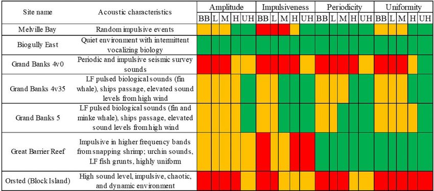
Wilford et al.                                                                                                       Quantitative Soundscape Analysis

signals are considered impulsive. Gaussian-distributed random              and is used to quantify envelope dissimilarity where s(f ) is
noise produces kurtosis values of 3.0. Time series with strong             the mean spectrum. Envelope dissimilarity is estimated between
sinusoidal signals have a kurtosis in the range of 0.0 to 3.0, and         two signals by computing the difference between their PMFs
time series with transients produce kurtosis values above 3.0              (Equations 11 and 12):
(Martin et al., 2020).
                                                                                                         n
    Cepstrum treats the log spectrum of a time series as a                                            1X
waveform, and the spectrum of this log spectrum produces                                       Dt =      | A1 (t) − A2 (t) |                    (11)
                                                                                                      2
                                                                                                        t=1
peaks when the original waveform contains echoes, or periodic
components (Oppenheim and Schafer, 2004). Cepstrum is                                                   n
                                                                                                      1X
calculated by taking the real part of the inverse discrete Fourier                             Df =       |S1 f − S2 f |                        (12)
transform (DFT) of the logarithm of the magnitude of the DFT                                          2
                                                                                                         t=1
of the signal (Equation 7):
                                                                           where A(t) is the PMF of the amplitude envelope and S(f) is PMF
                                                                           of the mean spectrum. D-index (Equation 13) is the product of

            Cepstrum = real IFFT log FFT pts                    (7)
                                                                           the temporal dissimilarity (Dt ) and spectral dissimilarity(Df ):
where pts is the pressure time series. Cepstrum was calculated
over averaged pressure time series using a built-in MATLAB                                             D = Dt × Df                              (13)
function rceps. However, the graphical output of cepstrum needed
                                                                           The D index is a between-group (β) index originally developed
to be further quantified for use in the soundscape code. To do
                                                                           to measure differences between communities. In the context
this, a threshold set at c(n) = 0.1 was chosen, and any peaks
                                                                           of this study, the D index is used to quantify differences in
above this threshold in the cepstrum output were used as proxies
                                                                           the soundscape across time by calculating it over consecutive
for periodicities with the number of peaks-per-minute (ppm)
                                                                           acoustic recordings.
counted and reported in the soundscape code.
                                                                              H-index (Equation 16) is the product of the spectral (Hf ) and
    Inspired by Martin et al. (2019), time lagged autocorrelation
                                                                           temporal (Ht ) entropies (Equations 14 and 15):
used to highlight periodicities in acoustic data was considered
as a periodicity metric candidate within the present study.                          n
                                                                                     X
Using an averaged pressure time series, the peaks above a                  Ht = −           A (t) × log2 (A (t)) × log2 (n)−1 , with Ht ε [0, 1]
selected threshold in autocorrelation plots can be counted and                        t=1
used as proxies for periodicity in a soundscape. Two averaging                                                                                  (14)
windows were assessed within this study to determine the best
fit for the soundscape code: 1.0 s mean square (MS) sound                             n
                                                                                      X
                                                                                            S f × log 2 (S f ) × log 2 (N)−1 , with Hf ε[0, 1]

pressure averages, and 0.1 s MS sound pressure averages. These              Hf = −
nuanced autocorrelation metrics are referred to as “acorr2”                           t=1
(1.0 s average), and “acorr3” (0.1 s average). The threshold for                                                                                (15)
periodicities using autocorrelation, a minimum peak prominence
of ρyy (t, t + τ) = 0.5, was set using the MATLAB function                                             H = Ht × Hf                              (16)
findpeaks, and any autocorrelation coefficient peaks in the 1-             where A(t) is the PMF of the amplitude envelope, and S(f) is
min time window above this threshold were counted (ppm). For               the PMF of the mean spectrum. H is 0 for a single pure tone,
acorr2, 45 (75%) lags were considered. For acorr3, 420 lags (70%)          increases with frequency bands and amplitude modulations, and
were considered.                                                           approaches 1 for random noise.
    The H and D indices are calculated using the amplitude
envelope which is given by the absolute value of the analytic signal
                                                                           Metric Performance Analysis
ζ(t), defined as (Equation 8):
                                                                           A qualitative analysis was done to determine the optimal
                      ζ (t) = p (t) + ipH (t)                 (8)          representative metric for each of the three soundscape properties
               √                                                           in the soundscape code. Visual analysis of spectrograms and
where: i =       −1, and ph (t) is the Hilbert transform of the            waveforms, coupled with knowledge of the sound sources present
real valued signal p(t). Probability mass functions (PMF) give             at each site, helped to form a priori expectations for the candidate
the probability that a discrete, random variable is exactly equal          soundscape metrics (Figure 3). Metric statistics were compared
to some value, and the PMF of the amplitude envelope A(t) and              against a priori expectations, identifying which metrics produced
PMF of the mean spectrum S(f) is given by (Equations 9 and 10):            the strongest agreement across soundscape code properties. The
                                                                           SPLpk and SPLrms metrics have been well studied as quantitative
                                      |ζ (t)|                              metrics of amplitude (Madsen, 2005; Thompson et al., 2013;
                            A (t) = Pn                          (9)
                                     t=1 |ζ (t)|                           Merchant et al., 2015) and further comparison was not deemed
                                                                           necessary. A series of qualitative comparisons (Table 4) were
                                     s(f)                                 used to inform the determination of which metric was optimal
                             S f = P                           (10)        for each property. The qualitative comparisons shown in Table 4
                                     n
                                           t=1      s(f                    do not represent an exhaustive review of the analysis completed

Frontiers in Marine Science | www.frontiersin.org                      7                                       August 2021 | Volume 8 | Article 672336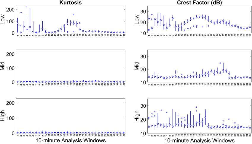
Wilford et al.                                                                                                     Quantitative Soundscape Analysis

using the soundscape code datasets, but rather represent the               rumbling acoustic activity dominated the lower frequencies
comparisons that produced definitive results in the analysis.              of the soundscape, but several instances of more broadband
Because amplitude metrics were already chosen, they are not                ice cracks exist in the dataset (Figure 2A). Impulsive metrics
featured among the list of comparisons.                                    were expected to reflect the presence of impulsive signals in
   The qualitative comparisons and time series analysis of the             mostly BB, Low, or Mid soundscape code bands. Kurtosis
candidate metrics informed most of the decision on which                   reported many values exceeding the impulsive threshold in
combination was optimal for use in the soundscape code.                    the BB, Low, and Mid soundscape code frequency bands
However, to explore how metric values could be used to                     indicating considerable impulsive acoustic activity in the
distinguish or draw comparisons between sites, some statistical            expected frequency bands (Figure 4).
analysis of the metric values and distributions respective                     Based on spectrogram analysis and an analysis of the
to each site and frequency band was desired. Because the                   sound pressure levels at MB, it was understood that while
ANOVA is an analysis specified for normally distributed                    potentially impulsive events occurred frequently throughout
Gaussian data, and distributions of kurtosis, D-index, and acorr3          the recording, a handful of high intensity events dominated
violated this assumption of normality, a non-parametric multiple           the soundscape. It was expected that the impulse metrics
comparisons for all site pairs using the Dunn method for joint             would reflect the sporadic and intermittent nature of the ice
ranking was utilized (Dunn, 1964). Multiple comparisons tests              cracks in boxplots of impulsiveness metric values through
were carried out using JMP ProTM 14.0.0 software and were                  greater variability (Figure 4). Kurtosis performed as expected
repeated for the Broadband, Low, Mid, and High frequency                   by indicating a wide range of kurtosis values that accurately
bands; for each frequency band analyzed, 21 site pairs were                captured the sporadic nature of the ice sounds. While crest
assessed. For each metric, groupings in respective frequency               factor reflected the presence of impulsive signals, it reported very
bands were formed by sites whose metric distributions were                 little distinction between the soundscape code frequency bands,
determined by the multiple comparisons tests to not be                     and the crest factor values varied much less than the kurtosis
significantly different. An assessment of how the candidate                values so that it was not as possible to detect that a handful of
metrics “grouped” the soundscapes highlighted how the different            high amplitude events characterized the impulsive nature of the
metrics would compare or contrast the soundscapes of similar               soundscape at MB.
and different acoustic environments. Connected letters reports                 At GB4v35, where the 20 Hz pulsed vocalizations formed the
were created for the multiple comparisons test results to better           basis for qualitative comparison I2, kurtosis values indicated the
visualize these groupings. Sites sharing common letters in the             presence of impulsive signals the in Low band for minutes 1, 2,
tables (within but not across frequency bands) have metric                 3, 5, 6, 7, 9, 10, 11 which corresponded closely to the minutes
distributions that are not significantly different (according to the       containing pulsed fin whale vocalizations. Mid and High band
Dunn method for joint ranking).                                            kurtosis values maintained values of 3 for the duration of the
                                                                           qualitative comparison I2. Crest factor peaks also aligned with the
                                                                           pulse trains, but unlike kurtosis, crest factor impulse detections
RESULTS                                                                    were identified in all soundscape code frequency bands, and for
                                                                           every minute but the 8th. The crest factor values in the Mid
Results from a series of comparisons that led to the final choice          (100–1000 Hz), High (1–10 kHz), and Ultra-High (>10 kHz)
of metrics are presented on a property-by-property basis. Results          soundscape code bands did not align with content visualized in
from several of the qualitative comparisons outlined in Table 4            the spectrograms or a priori expectations made based on the
are presented to highlight the responses that guided the metric            knowledge that the dominant sound source at this site was fin
selection. Metric comparisons were conducted for impulsiveness,            whales. However, 3–10 dB fluctuations in the 1-second SPLpk
periodicity, and uniformity properties. As stated previously,              in the Ultra-high band were detected, which could indicate the
metrics for amplitude were already identified from previously              presence of an impulsive sound and justify the higher than
published work as well-established and effective measures of               expected crest factor values (see Supplementary Figure 1 related
the amplitude of sound pressure, so they were selected for                 to qualitative comparison I2). Ten-min boxplots were used to
the soundscape code without further analysis (Madsen, 2005;                explore how the metric values changed over time at GB4v35
Thompson et al., 2013; Merchant et al., 2015). Calculated metric           (Figure 5). Crest factor (Figure 5 Right) remained high during
time series were compared to spectrograms, pressure waveforms,             the period of ship noise (box 10–11), so it was difficult to
and a priori expectations to guide final metric selection.                 deduce from the crest factor values that a ship had contributed
                                                                           significantly to the soundscape. In contrast, kurtosis values
Impulsiveness                                                              (Figure 5 Left) dropped quickly after the introduction of vessel
Both kurtosis and crest factor were generally found to accurately          noise to the soundscape (box 10–11), and values only increased
report the presence of impulsive signals. However, kurtosis                after the vessel noise had subsided and the soundscape returned
values more closely aligned with a priori expectations in                  to being dominated by the pulsed signals of the fin whales (boxes
characterizations of the impulsiveness of the soundscape code              14–21). Kurtosis also only showed a slightly elevated response
datasets. The superiority of kurtosis in indicating the presence           to a different fin whale chorus that correspond roughly to boxes
of impulsive signals was suggested in qualitative comparison               22-32 and a different recording period. Crest factor indicated
I1, which featured sound from only one dominant sound                      little difference between the impulsiveness of the two different
source: ice. Spectrograms showed that ice cracks, groans, and              fin whale choruses.

Frontiers in Marine Science | www.frontiersin.org                      8                                     August 2021 | Volume 8 | Article 672336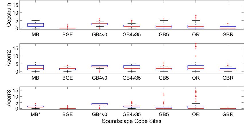
Frontiers in Marine Science | www.frontiersin.org
Wilford et al.
TABLE 4 | Qualitative comparisons of soundscape code property metrics and summary of results.
I.D. Site Data represented Test basis Expectations Summary of Results
Qualitative Melville Bay (MB) Iceberg noise The entirety of the recording was Intermittent levels of impulsiveness in Kurtosis outperformed crest factor by
comparison I1 considered in this test. frequency bands associated with the ice indicating frequency of dominant signals of
(Impulsiveness) noise (Low, Mid, decaying in High) ice sounds more appropriately
Qualitative Grand Banks Fin whale Two consecutive 10-min time windows Metrics should indicate high levels of Kurtosis outperformed crest factor by
comparison I2 Station 4 (GB4v35) were considered. (1) contains two full and impulsiveness in the low band in time indicating frequency of dominant signals of
(Impulsiveness) one partial fin whale pulse train. (2) contains window 1, and reduced level in time fin whale vocalizations more appropriately
no pulse trains. window 2.
Qualitative Grand Banks Seismic survey Two 10-min time windows were Metrics should indicate high levels of Kurtosis outperformed crest factor. Kurtosis
comparison I3 Station 4 (GB4v0) considered: (1) sounds from distant impulsiveness in only the low, mid, and high results indicated frequency of dominant
(Impulsiveness) seismic, (2) sounds from close proximity bands, and report an increase in signals of seismic survey signals and
seismic. impulsiveness value in time window 2. highlighted the difference in strength of
seismic signals more accurately.
Qualitative Grand Banks Fin Whale Identical subsets used in I2 Metrics should report a decrease in Cepstrum and acorr3 outperformed acorr2
comparison P1 Station 4 (GB4v35) periodicity from time window 1 to time and accurately reported decreased
9
(Periodicity) window 2. periodicity of signals contained in second
time window.
Qualitative Grand Banks Seismic Survey Identical subsets used in I3 Metrics should report increase in periodicity All three periodicity metrics performed
comparison P2 Station 4 (GB4v0) from time window 1 to time window 2. similarly and accurately report increased
(Periodicity) periodicity of signals in time window 2.
Qualitative Orsted (OR; Block Pile Driving Two 10 min time window were considered: Metrics should report a decrease in All three periodicity metrics performed
comparison P3 Island) (1) periods of intense and repetitive pile periodicity from time window 1 to time similarly and accurately report decreased
(Periodicity) driving sounds, (2) no pile driving window 2. periodicity of signals in time window 2.
Qualitative Melville Bay and Chaotic ice Two full recordings. Metrics must reflect Metrics should reflect sporadic nature of ice D-index outperformed H-index and
comparison U1 Biogully East sounds/quiet acoustic uniformity within site and between sounds in contrast to mostly consistent accurately contrasted acoustic uniformity at
(Uniformity) environment sites. nature of BGE soundscape MB and BGE.
Qualitative Orsted and Great Chaotic pile driving, Two entire recordings were considered for Metrics should indicate the GBR is more Both metrics performed similarly but the
comparison U2 Barrier Reef ship noise, dolphin U2. Methods utilized in U2 identical to U1. consistent. Indication of presence of range measure of the D-index provided an
August 2021 | Volume 8 | Article 672336
(Uniformity) whistles/reef sounds common dolphin vocalizations at OR, and accurate assessment of the different sites.
fish grunts at GBR are a secondary Difference in responses was nuanced but
Quantitative Soundscape Analysis
expectation. favored D-index.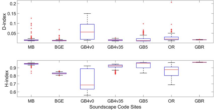
Wilford et al.                                                                                                                         Quantitative Soundscape Analysis

  FIGURE 3 | A priori metric response expectations for each data set. Expectations formed criteria to compare metrics and inform the metric selection.
  Green-Yellow-Red coloration represents relative expected metric response level where green indicates a low property level, yellow indicates a mid-level, and red
  indicates high-level responses. Low-level responses for the uniformity category indicate a uniform acoustic environment, and high-level responses indicate a lack of
  uniformity. Corresponding soundscape code frequency band is indicated by abbreviations for Broadband (BB), Low (L), Mid (M), High (H), Ultra-High (UH).

  FIGURE 4 | Impulsiveness comparison I1 results for (A) kurtosis and (B) crest factor. Wherein the boxplots red horizontal line indicates median value, outer edges of
  boxes represent 25th and 75th percentiles, whiskers mark boundary that contains approximately 99% of data values, and the red points are outliers.

   Qualitative comparison I3 which contained signals from                               Periodicity
a seismic survey (Figure 2B) yielded similar results in                                 Periodicity metrics all reflected aspects of the periodic nature
terms of the performance of the two impulsiveness metrics.                              of each of the soundscapes and differences in metric responses
Ultimately, both metrics adequately reported the nature of the                          were typically nuanced (Figure 6). Acorr3 was found to be more
impulsive seismic survey signals, but kurtosis again aligned                            closely linked to the periodic nature of the soundscapes, and was
more with the salient signals in the proper frequency bands                             more robust to mischaracterizations of the soundscapes that were
(see Supplementary Figure 2 related to qualitative comparison                           observed with acorr2 and cepstrum.
I3). 10-min boxplots of both crest factor and kurtosis values                              In comparison P1, subsets of the GB4v35 dataset contained
adequately reflected the nature of the impulsive signals in                             unequal numbers of fin whale pulsed vocalizations, and this
the GB4v0 soundscape. However, kurtosis boxplots at GB4v0                               disparity was used to compare the responses of the periodicity
highlighted the difference in seismic survey signals as the survey                      measures to determine if the metrics would report more peaks in
vessel approached, passed over the hydrophone, and departed.                            time window 1, which contained far more of the 20 Hz periodic
Crest factor, on the other hand, indicated little difference between                    fin whale vocalizations (Figure 7). Cepstrum reported 27 fewer
the phases of the survey.                                                               peaks across frequency bands in time window 2, while acorr3

Frontiers in Marine Science | www.frontiersin.org                                  10                                           August 2021 | Volume 8 | Article 672336
Wilford et al.                                                                                                                        Quantitative Soundscape Analysis

  FIGURE 5 | Boxplots of kurtosis values for the Low (A), Mid (B), and High (C) bands and crest factor values for the Low (D), Mid (E), and High (F) bands at
  GB4v35. Each box represents the range of metric values in a 10-min time window comprised of metrics calculated over 1-min time windows (each boxplot contains
  10 metric values). Circled dots intersecting boxes indicate median values, thick boxes indicate 25th and 75th percentile range, narrower lines indicate range of 99%
  of data, and blue circles indicate outliers.

  FIGURE 6 | Broadband periodicity candidate metric results for all soundscape code datasets. Values represent peaks-per-minute as reported by (A) cepstrum, (B)
  acorr2, and (C) acorr3. The red horizontal line indicates the median value, outer edges of boxes represent 25th and 75th percentiles, whiskers mark the boundary
  that contains approximately 99% of data values, and the red points are outliers.

reported 11 fewer peaks. In a deviation from expectations, acorr2                         Qualitative comparisons P2 and P3 yielded results that were
reported six more peaks for the second time window.                                    less conclusive than P1. Comparison P2 utilized sounds from
    Time series analysis using 10-min boxplots over the entirety of                    a seismic survey (Figure 2B) and metrics were expected to
the GB4v35 dataset similar to the analysis presented in Figure 5                       report an increase in peaks-per-minute from time window 1
showed two main differences: (1) Acorr2 reported more peaks                            to time window 2. Time window 1 captured distant seismic
per minute than acorr3 in the High band for 69% of the minutes                         survey signals, while time window 2 captured close proximity
analyzed (n = 353). (2) Both acorr2 and acorr3 were highly                             signals that were louder and had more consistent repetition.
consistent during the second period of fin whale vocalizations                         All metrics reported more peaks-per-minute across Soundscape
while cepstrum varied more (see Supplementary Figure 3 related                         Code frequency bands for the second time window of the GB4v0
to time series analysis of the periodicity metrics at GB4v35).                         dataset. Comparison P3 utilized the sounds from an impact pile

Frontiers in Marine Science | www.frontiersin.org                                 11                                           August 2021 | Volume 8 | Article 672336
Wilford et al. Quantitative Soundscape Analysis
FIGURE 7 | Periodicity comparison P1 results. 20-Hz fin whale vocalizations captured in (A) frequency filtered 1-SPLpk for time window 1 (left) and time window 2
(right). Boxplots show range of periodicity candidate metric values (ppm) corresponding to the two time windows for (B) cepstrum, (C) acorr2, and (D) acorr3. The
red horizontal line indicates the median value, outer edges of boxes represent 25th and 75th percentiles, whiskers mark the boundary that contains approximately
99% of data values, and the red points are outliers.
driving operation (Figure 2D) and metrics were expected to representation of the acoustic activity of northern bottlenose.
report a decrease in peaks-per-minute from time window 1 to Disruption of acoustic uniformity from the northern bottlenose
time window 2. Time window 1 featured intense pile driving whales at BGE was reflected clearly in time series analysis of
sounds and time window 2 did not. The periodicity metrics in D-index values. H-index also reflected the decreased uniformity
P3 reported a substantial decrease in peaks-per-minute across the at MB, but the dependence of this metric on bandwidth
two time windows. 10-min boxplots of periodicity metrics plotted made interpretation and comparison difficult, as H-index values
over the duration of the datasets used in qualitative comparisons increased from the Low to Ultra-High soundscape code band
P2 and P3 did not indicate conclusive differences and all metrics regardless of acoustic uniformity. D-index soundscape code
responded appropriately to the different acoustic activity featured values in Figure 9 reflect the substantial disparity in acoustic
in the two datasets. uniformity between the two sites in both magnitude and
variability of the index. In contrast, the slightly larger range of
Uniformity the H-index values corresponding to the MB Low band indicated
D-index values aligned with a priori expectations and only a slight disparity in acoustic uniformity between the two
outperformed the H-index in every analysis conducted using the sites, and the magnitude of the index was not representative of
soundscape code datasets. D-index values accurately captured the recording content.
the acoustic uniformity at all soundscape code datasets by Similar analysis carried out on data from the OR and GBR
indicating consistently high values at GB4v0 and OR, and the sites yielded slightly different results. In qualitative comparison
presence of high values in sites where dramatic changes in the (U2), comparisons of respective uniformity metrics across the
acoustic environment occurred (Figure 8). sites highlights differences in acoustic uniformity. D-index values
Comparisons of uniformity metric results drew on ice sounds more clearly capture the disparity in acoustic uniformity between
from MB (Figure 2A), pile driving and boat noise from OR OR and GBR especially in the increased size of the boxplots of
(Figure 2D), reef sounds from GBR (Figure 2G), and sporadic values at OR in the High and Ultra-High bands. H-index values
echolocation and whistling activity from BGE (Figure 2E) to used to compare the acoustically distinct OR and GBR sites failed
determine which metric would represent soundscape uniformity to reflect the acoustic disparity by producing almost identical
in the soundscape code (Table 4 rows 7 and 8). At MB, soundscape code medians, with only slightly more variability of
the D-index values in the low and mid bands reflected the the 1-min H-index values reported at OR. Similar to the H-index,
sporadic and random ice noise (Figure 9). Compared to BGE, the magnitudes of the D-index values at both OR and GBR were
D-index values accurately characterized MB as more variable in only slightly different. The variability measure of the D-index,
these bands. In the High and Ultra-High bands, BGE D-index however, did reflect the disparity in acoustic uniformity across
values were greater than MB, which again was an accurate OR and GBR (see Supplementary Figure 4 figure related the
Frontiers in Marine Science | www.frontiersin.org 12 August 2021 | Volume 8 | Article 672336Wilford et al. Quantitative Soundscape Analysis FIGURE 8 | Broadband (A) D-index and (B) H-index metric values for all seven soundscape code sites. Red horizontal line indicates median value, outer edges of boxes represent 25th and 75th percentiles, whiskers mark boundary that contains approximately 99% of data values, and the red points are outliers. FIGURE 9 | Uniformity comparison U1 results. H-index values for (A) BGE and (C) MB sites; D-index values for (B) BGE and (D) MB sites; Red horizontal line indicates median value, outer edges of boxes represent 25th and 75th percentiles, whiskers mark boundary that contains approximately 99% of data values, and the red points are outliers. Corresponding soundscape code results for (E) the D-index at BGE and MB, and (F) the H-index at BGE and MB report the median (med) and size of the 95% confidence interval (CI95). qualitative comparison U2). When metric values were analyzed H-index suggested D-index was the optimal metric to represent using 10-min boxplots over the full OR recording, the D-index acoustic uniformity in the soundscape code. more effectively captured the dynamic nature of the soundscape, while the H-index values hardly indicated any changes in acoustic Statistical Groupings of Metric Values activity (see Supplementary Figures related time series analysis The non-parametric multiple comparisons tests were used to of the uniformity indices at OR and GBR). The intuitive nature form the statistical groupings of sites based on the medians of the of the D-index and much closer alignment to salient acoustic metric values (Figure 10). Respective to each site, metric values activity in the soundscapes of the soundscape code datasets than that are not significantly different are “connected” by identical Frontiers in Marine Science | www.frontiersin.org 13 August 2021 | Volume 8 | Article 672336
Wilford et al.                                                                                                      Quantitative Soundscape Analysis

letters in the connected letter tables that report the multiple             allowed comparisons of the soundscape code datasets to be
comparisons results. In key frequency bands, the uniquely                   made in terms of sound amplitude, impulsiveness and transient
impulsive soundscapes of MB, GBR, OR, and GB4v0 were all                    events, content of repetitive signals, and spectral and temporal
found to have kurtosis values that were significantly different than        variability. For example, in a comparison of the impulsiveness
the sites where impulsive signals were either rare or only faint            of the soundscape code datasets GB5, GB4v35, and BGE,
(BGE, GB4v35, and GB5) (Figure 10A). Kurtosis was observed                  impulsiveness metric values indicate they are the least impulsive
to outperform crest factor in terms of robustness, sensitivity,             sites of the seven (Figure 11). This observation was made
and more informative soundscape grouping, which led to the                  quickly, and demonstrates the ease with which one can compare
selection of kurtosis to represent impulsiveness in the soundscape          and contrast different soundscapes when identical metrics are
code. Periodicity metrics failed to produce intuitive groupings             being compared. This assessment of across site impulsiveness
of the sites in terms of periodic content, and acorr3 was the               can be taken a step further: The elevated 95% CI value in the
only metric that produced significantly different values between            Ultra-High (relative to BB, Low, Mid, and High) band at BGE
the highly periodic site and the moderate-low periodic sites                indicates the presence of acoustically active northern bottlenose
(MB, BGE, GB5, and GBR) (Figure 10B). In spite of less than                 whales. At the same time, the median and 95% CI in the Low
ideal groupings for acorr3, optimal performance in qualitative              bands at GB4v35 and GB5, respectively, indicate the presence
comparisons and other analyses made it the only viable choice               of chorusing fin whales. Martin et al. (2020) showed that 1-min
and acorr3 was selected as the metric to represent soundscape               kurtosis values increased as the amplitude of simulated impulses
periodicity. Multiple comparisons results for the D-index were              increased, so the slightly elevated impulsiveness metric values
both adequate and less than ideal, depending on which frequency             at GB4v35 relative to GB5 could be a manifestation of the
band was being considered (Figure 10C). However, considering                higher amplitude of the fin whale chorus at GB4v35, and this
the far more intuitive nature of the index and consistently better          coincides with increased SPLpk values at this site. This example
performance relative to the H-index, D-index was chosen to                  highlights how a combination of multidimensional metrics
represent acoustic uniformity in the soundscape code.                       can be used congruently to understand a soundscape and how
                                                                            nuanced differences in the metrics can indicate significant
                                                                            differences in soundscape composition. The collection of metrics
DISCUSSION                                                                  captures temporal and frequency characteristics of acoustic
                                                                            environments and depending on application can be used to
A collection of metrics was applied to a series of unique                   assess spatial temporal and variation in soundscapes directly
soundscapes to identify the optimal suite of metrics for capturing          corresponding to the soundscape components defined in ISO
the salient soundscape characteristics, which ultimately enables            (2017) 18405.
quick and simple quantitative comparisons of soundscapes.                       The proposed soundscape code provides a valuable framework
The final determination considered both the metric efficacy in              to simply covey complex ocean characteristics and is a “first
quantifying the corresponding soundscape property, and how                  step” in the direction of a standardized soundscape analysis
well the metric fit into the infrastructure of the soundscape               and reporting structure. We recognize that the future use and
code. SPLrms and SPLpk (amplitude), kurtosis (impulsiveness),               potential improvement of the soundscape code will benefit
D-index (uniformity), and acorr3 (periodicity) were determined              from more thorough assessment of duty cycling, bandwidth
to be the best metrics out of the candidate metrics for comparing           definitions, and dataset durations, as only data sets of multiple
soundscapes. Soundscape codes comprised of the optimal metrics              hours and a majority of continuous sampling regimes were
indicated dominant signal frequencies and salient differences in            used to select the proposed soundscape code metrics. Further
acoustic environments (Figure 11). Figure 11 represents what                work assessing the impact and performance of different analysis
an initial soundscape assessment using the soundscape code                  windows (larger time scales), datasets with unique acoustic
methodology might look like; tabulated soundscape information               features not captured in this work, datasets with significant
across frequency bands and metrics offers an initial “glimpse”              overlapping of source signals, and threshold selections is required
into a marine acoustic environment and highlights areas of                  to ensure the development of an effective, rapid, and robust
interest for further targeted analysis. The soundscape code is              quantitative soundscape framework.
proposed here as a first step in the direction of a standardized                Duty cycle was found to have impacts on the D-index, as the
soundscape analysis methodology that will ultimately facilitate             D-index measures the difference between consecutive recordings,
quantitative comparison and assessment of soundscapes, and                  and consecutive recordings will have more in common than
guide subsequent analysis.                                                  recordings spaced apart by longer periods of time. The selected
   Traditionally, underwater soundscape studies focus                       frequency bandwidths worked for the purposes of this project,
mostly on quantifying fluctuations, central tendencies, or                  but other frequency banding should be explored to better
minimum/maximum observed levels of amplitude typically                      represent evolving regulations and knowledge of marine life
represented by sound pressure, intensity, or acoustic energy                hearing. Similar to duty cycle concerns, dataset duration being
(Table 1). If metrics that quantify aspects of other soundscape             represented in the soundscape code should be explored to
properties are included in soundscape analysis, a more thorough             understand how a comparison of soundscape code results from
assessment of soundscapes is possible. The soundscape properties            a small duration dataset (minutes to hours) compares to results
outlined in Table 2 were quantified by the selected metrics, which          from a large duration datasets (days to months). A final aspect to

Frontiers in Marine Science | www.frontiersin.org                      14                                     August 2021 | Volume 8 | Article 672336
You can also read