Machine Learning Implicit Solvation for Molecular Dynamicsa
←
→
Page content transcription
If your browser does not render page correctly, please read the page content below
Machine Learning Implicit Solvation for Molecular Dynamicsa)
                                                            Yaoyi Chen,1 Andreas Krämer,1 Nicholas E. Charron,2, 3, 4 Brooke E. Husic,1, b) Cecilia Clementi,4, 3, 5, 2, c) and
                                                            Frank Noé1, 5, 4, d)
                                                            1)
                                                               Department of Mathematics and Computer Science, Freie Universität, Berlin,
                                                            Germany
                                                            2)
                                                               Department of Physics, Rice University, Houston, Texas 77005, USA
                                                            3)
                                                               Center for Theoretical Biological Physics, Rice University, Houston, Texas 77005,
                                                            USA
                                                            4)
                                                               Department of Physics, Freie Universität, Berlin, Germany
                                                            5)
                                                               Department of Chemistry, Rice University, Houston, Texas 77005, USA
                                                            (Dated: last built on June 15, 2021)
arXiv:2106.07492v1 [physics.comp-ph] 14 Jun 2021

                                                            Accurate modeling of the solvent environment for biological molecules is crucial for computational biology and
                                                            drug design. A popular approach to achieve long simulation time scales for large system sizes is to incorporate
                                                            the effect of the solvent in a mean-field fashion with implicit solvent models. However, a challenge with existing
                                                            implicit solvent models is that they often lack accuracy or certain physical properties compared to explicit
                                                            solvent models, as the many-body effects of the neglected solvent molecules is difficult to model as a mean
                                                            field. Here, we leverage machine learning (ML) and multi-scale coarse graining (CG) in order to learn implicit
                                                            solvent models that can approximate the energetic and thermodynamic properties of a given explicit solvent
                                                            model with arbitrary accuracy, given enough training data. Following the previous ML–CG models CGnet
                                                            and CGSchnet, we introduce ISSNet, a graph neural network, to model the implicit solvent potential of mean
                                                            force. ISSNet can learn from explicit solvent simulation data and be readily applied to MD simulations. We
                                                            compare the solute conformational distributions under different solvation treatments for two peptide systems.
                                                            The results indicate that ISSNet models can outperform widely-used generalized Born and surface area models
                                                            in reproducing the thermodynamics of small protein systems with respect to explicit solvent. The success
                                                            of this novel method demonstrates the potential benefit of applying machine learning methods in accurate
                                                            modeling of solvent effects for in silico research and biomedical applications.

                                                   I.   INTRODUCTION                                                    solvent implicitly has several advantages: it can speed up
                                                                                                                        force calculations by drastically reducing the the num-
                                                      The solvent environment around macromolecules of-                 ber of degrees of freedom; it increases the effective time
                                                   ten plays a significant, sometimes even decisive, role in            step size in MD simulations;17 and it simplifies constant-
                                                   both the structure and dynamics of biological systems.1–3            pH simulations18,19 as well as enhanced sampling ap-
                                                   For example, the so-called “hydrophobic core”, a key                 proaches, such as parallel tempering (PT)/replica-
                                                   structural element shared by a diverse variety of protein            exchange MD.20,21 Moreover, implicit solvent treatment
                                                   domains strongly influences protein folding in aqueous               is very common in structure-based drug design, such as
                                                   solution.4,5 The solvent also renders the protein structure          fragment screening and lead optimization.22,23 Some gen-
                                                   flexible enough for functional conformational changes6               eralized Born (GB)-based implicit solvent methods, for
                                                   and mediates interactions among macromolecules for bi-               example, are implemented in various MD software pack-
                                                   ological processes4,7 as well as drug binding.8–10                   ages, such as GBSA–HCT,24 GBSA–OBC and GBn mod-
                                                      Thus, for computational investigations of biomedical              els25 in AMBER,26 GBMV27,28 and GBSW models29 in
                                                   problems, such as molecular dynamics (MD) simulations                CHARMM.30 Ref. 31 gives an comprehensive comparison
                                                   of biological systems11–13 and molecular docking,14 we               of available implicit solvent models.
                                                   often seek to accurately model effects of the solvent envi-             Despite their advantages, the accuracy of commonly
                                                   ronment. In MD simulations, solvation methods can be                 used implicit solvent models tends to be inadequate in
                                                   grouped into two major categories: explicit and implicit.            certain applications, such as the calculation of solva-
                                                   The former incorporates solvent molecules explicitly into            tion free energies32 or the recovery of correct confor-
                                                   the simulation system, while the latter represents sol-              mational distributions for folded and unfolded states of
                                                   vent effects in a mean-field manner.11,15,16 Treating the            proteins,33–35 thereby limiting their usage and effective-
                                                                                                                        ness in practice.
                                                                                                                           The present work addresses a long-standing question
                                                                                                                        in solvent modeling: is it possible to construct mean-field
                                                   a) This article has been submitted to the Journal of Chemical        implicit solvent models that reproduce the solvation ther-
                                                   Physics.                                                             modynamics of explicit-solvent systems exactly? We ap-
                                                   b) Corresponding author; Electronic mail: husic@princeton.edu        proach this problem by parameterizing implicit solvent
                                                   c) Corresponding author; Electronic mail:     cecilia.clementi@fu-   models via a machine-learned coarse graining approach.
                                                   berlin.de                                                            Coarse graining of molecular systems is itself a well-
                                                   d) Corresponding author; Electronic mail: frank.noe@fu-berlin.de
                                                                                                                        researched topic, one whose aim is to model molecules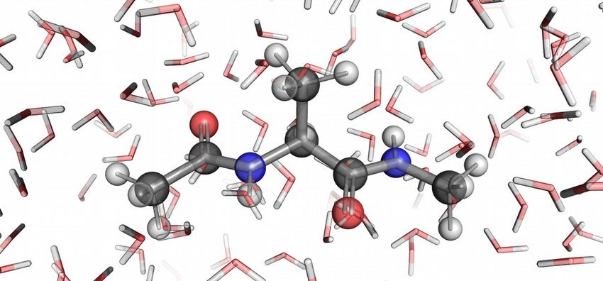
2
and their interactions with super-atomistic resolutions,
such that computational investigations (e.g., MD simula-
tions) become more efficient.36–48 A coarse grained (CG)
model usually entails two important aspects: the CG
resolution and representation—that is, the mapping of
the original atoms into effective interacting groups (also
known as CG beads)39,41,42,49,50 —and the CG poten-
tial, which determines the interactions among the CG
beads.39,41,42 Here we consider an implicit solvent system (a)
as a CG version of the explicit solvent system—the CG
mapping keeps the solute molecule(s) while removing the
solvent degrees of freedom. Once the CG mapping has (b)
been assigned, the parameterization of a CG potential
may follow either a “top-down” approach; i.e., one that
aims at reproducing macroscopic experimental observa-
tions, or a “bottom-up” strategy, which systematically
integrates information from the corresponding atomistic
system.39 In this work we leverage the multi-scale coarse
graining theory,51,52 a “bottom-up” approach. Essen-
tially, it transforms the parameterization of a CG po-
tential into a data-driven optimization based on the vari-
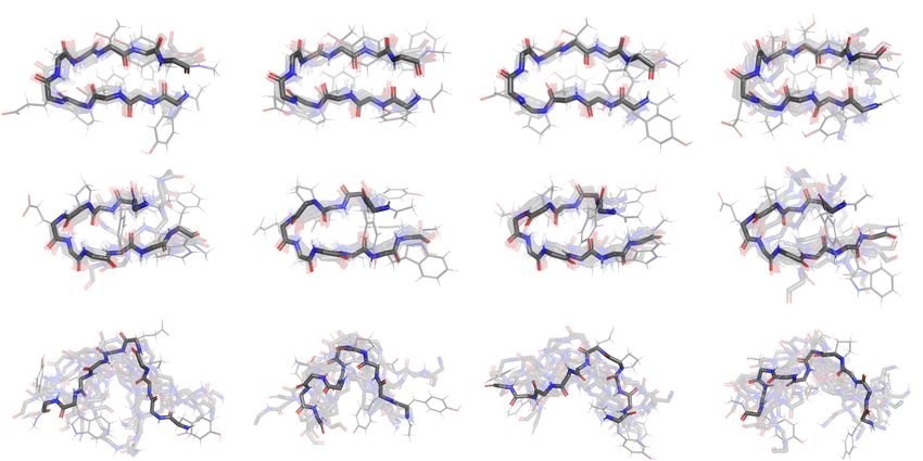
ational force matching (FM) method. Figure 1. Explicit (above) and implicit (below) solvation
The multi-scale coarse graining theory enables us to treatment of a biomolecular system (here we use capped ala-
nine as an example).
employ a machine learning method similar to the CGnet
introduced by Wang et al.46 to learn an implicit sol-
vent model, which is part of the CG potential for the
solute, for any given molecular system. Machine learn- ral network architecture, training and validation as well
ing methods have enjoyed increased in popularity and as implicit solvent simulation. In the Results we apply
led to breakthroughs in many fields,53 including molec- our proposed method to two molecular systems—capped
ular sciences.54–57 For structural coarse graining in par- alanine (Fig. 1) and the miniprotein chignolin.66 We show
ticular, there have been some pioneering works both for that our method can reproduce the solvated thermody-
choosing optimal CG mappings50,58 and for parameter- namics with higher accuracy than a reference implicit
izing CG potentials for a given system.46,48,58–60 In this solvent method, namely the GBSA–OBC model.67 In the
work, we adapt the architecture of CGnet46 and its exten- Discussion section we address the current limitation and
sion CGSchNet48 (the latter based on a graph neural net- future investigative directions of the ISSNet method.
work architecture SchNet61 ) to the implicit solvent prob-
lem. The resulting implicit-solvent SchNet—henceforth
called ISSNet—is able to learn an implicit solvent model II. THEORY AND METHODS
from coordinate and force samples of a corresponding ex-
plicit solvent system. Trained ISSNet models can in turn Here, we introduce the potential of mean
be used for implicit solvent simulations of biomolecules. force (PMF)—a concept from statistical mechanics—as
Recently, machine learning methods have been applied a theoretical basis both for implicit solvent methods
in some studies related to solvent environment, such as and for the multi-scale coarse graining theory. After
the automatable cluster-continuum modeling of the sol- examining how a traditional approach approximates the
vent in quantum chemistry calculations,62 for the param- implicit solvent PMF, we adapt an established machine
eterization of CG water models for ice-water mixture63 learning CG method for parameterizing implicit solvent
and liquid water systems,64 and for the computation of models based on explicit solvent simulation data.
generalized Born radii in implicit solvent simulations.65
The latter three studies are applicable to MD simula-
tions; however, the goal is either to achieve higher accu- A. Solute PMF and solvation free energy
racy for water-only systems or to improve the efficiency
of an existing method. This work distinguishes itself The concept of PMF originated in a 1935 paper
from existing studies by introducing a neural-network- by J. G. Kirkwood on statistical treatment of fluid
based implicit solvent method for biomolecular MD sim- mixtures.68 In this subsection we derive the expression
ulations. of a solute PMF following the framework of Ref. 69.
The paper proceeds as follows: we first describe Suppose we have an explicit solvent all-atom molecu-
the theoretical basis of implicit solvent treatment with lar system with a total number of N atoms, consisting of
ISSNet as well as the implementation, including the neu- Nmol solute atoms with coordinates r (e.g., biomolecule)
3

and (N − Nmol ) solvent atoms with coordinates w (e.g.,       denotes the forces on solute coordinates r with the solvent
water atoms and ions). Usually, an all-atom molecular         conformation being w, and
mechanics force field, such as AMBER26 or CHARMM,30                                     Z
formulates a molecular potential function v(r, w) as a                          h·ir := dw · p(r, w)
sum of bonded and non-bonded terms.11,13 Therefore,
without loss of generality, we can decompose v(r, w)
into three partial sums:69 vmol (r) for interactions solely   is a marginal operator that averages over all solvent con-
within and between the solute molecule(s), vw (w) for         figurations consistent with a given solute configuration
those solely within and between solvent molecules and         according to the Boltzmann distribution p(r, w).
vmw (r, w) for solute-solvent interactions:                      Theoretically, if we have V (r) as defined in Eq. (5) in
                                                              the first place, then we can directly sample P (r) as in
        v(r, w) = vmol (r) + vw (w) + vmw (r, w).      (1)    Eq. (3) and analyze most biologically relevant processes,
                                                              where solvent coordinates can be ignored (e.g., protein
We will refer to the solute-only potential vmol (r) as the    folding, protein-ligand binding or in general any observ-
“vacuum potential”, since it only consists of terms that      able defined by a function of the solute conformations
describe the solute molecule(s) in vacuum.                    only).69 However, in most cases we cannot solve the in-
  For a chosen thermodynamic state (e.g., with fixed          tegral in Eq. (5) analytically.
number of atoms N , volume V and temperature T in a              Alternatively, one can try to construct an approxima-
canonical ensemble), the equilibrium probability density      tion to the exact PMF, which is usually determined by
p(r, w) for a solute-solvent configuration r, w is:           first fixing a range of candidates with fixed functional
                                                              forms {V (r; Θ)} and then optimizing the parameter Θ.
                             e−βv(r,w)
             p(r, w) = R     R             ,           (2)    An often adopted decomposition in the parameterization
                           dr dw e−βv(r,w)                    is to separate the vacuum potential from the solvent-
where the scaling factor β depends on the thermody-           solvent and the solute-solvent interactions. Applying
namic ensemble used. In the canonical (NVT) ensem-            Eq. (1) to Eq. (5), we can move vmol (r) out of the in-
ble at temperature T it is given by β := 1/(kB T ) with       tegral and thus
Boltzmann constant kB . The distribution p(r, w) can be
                                                                               V (r) = vmol (r) + Vsolv (r),          (8)
sampled as a whole by MD or Monte Carlo simulations
with the explicit solvent potential v(r, w).
                                                              in which the solvation free energy Vsolv is defined as a
   For implicit solvent models, we are interested in recov-
                                                              function of solute configuration
ering a potential that describes the distribution of the
solute molecules only. The density associated with this                             Z
potential is formed as the marginal density obtained by       Vsolv (r) := −β −1 ln    dw e−β[vw (w)+vmw (r,w)] + const.
integrating over the solvent degrees of freedom:
                                                                                                                    (9)
                                                              Since the vacuum potential vmol (r) is known a priori
                           Z
                   P (r) := dw p(r, w).                 (3)   from the all-atom force field, we can write any candidate
                                                              for approximating the solute PMF V (r) in the following
We seek a potential function of solute coordinates V (r)      form:
that could generate the marginal distribution P (r). In
other words, the potential V (r) should satisfy the follow-                V (r; Θ) := vmol (r) + Vsolv (r; Θ),      (10)
ing equation:
                                                              and optimizing V (r; Θ) is equivalent to finding the best
                    e−βV (r)                                  approximation Vsolv (r; Θ∗ ) to the solvation free energy
                                = P (r).               (4)
                                                              as defined in Eq. (9). Vsolv (r; Θ∗ ) is an implicit solvent
                  R
                    dr e−βV (r)
                                                              model, since it does not explicitly involve any solvent, but
By inserting Eq. (2) and (3) and solving for V (r), we        can be used to approximately sample the Boltzmann dis-
have                                                          tribution of solute conformations by taking into account
                                                              the solvent environment implicitly according to Eq. (4).
                      Z
                 −1
      V (r) = −β ln      dw e −βv(r,w)
                                         + const.   (5)

V (r) is the so-called solute PMF,68,69 because its force     B.   Traditional implicit solvent models
corresponds to the mean force on the solute coordinates:
                                                                 A widely used strategy for parameterizing implicit sol-
            F(r) := −∇r V (r) = hfr (r, w)ir ,         (6)    vent models is to decompose the solvation free energy
                                                                                                           np
where                                                         (Eq. (9)) into two terms: the non-polar Vsolv   and the
                                          T                 electrostatic (polar) Vsolv contributions
                                                                                      elec

                           ∂v           ∂v
            fr (r, w) := −     ,··· ,−                 (7)                                 np
                           ∂r1         ∂rN                                   Vsolv (r) = Vsolv         elec
                                                                                               (r) + Vsolv  (r),     (11)
4
and seek approximations for both terms separately (de- Consider a CG mapping Ξ that treats each solute atom
tails can be found in Ref. 69). Various models have in a system as a “CG particle”:
been developed based on generalization of simple physical
models and/or heuristics70–72 for each of the two terms.
r INmol
r=Ξ , Ξ= , (14)
Here we illustrate Eq. (11) through an example of the w 0
popular generalized Born models.70–72 As the name sug-
gests, these models employ an approximation to the elec- where this linear transformation essentially truncates the
trostatics by generalizing the Born model73 for charged coordinates by eliminating the solvent degrees of free-
spherical particles (e.g., simple ions): dom. It is straightforward to show that the CG system
defined by the mapping Ξ can be treated under the multi-
scale coarse graining framework, and the solute PMF
1 1 1 X qi qj
elec
Vsolv,GB = − , (12a) defined by Eq. (4) is a CG PMF with thermodynamic
2 out in i,j fij
consistency.52 Moreover, the mean force, F(r), acting on
the solute (as derived in Eq. (6)) is a CG mean force.
s
in which fij = rij 2 + B B exp − rij , (12b)
i j
4Bi Bj More than merely a change of notation, treating the
implicit solvent system as a CG system of the explicit
one enables us to apply the variational FM method for
where out and in are outer and inner (regarding the gen-
parameterizing an implicit solvent model. For each can-
eralized Born sphere) dielectric constants, respectively.
didate potential function V (r; Θ), the multi-scale coarse
Parameters {qi }, {rij } and {Bi } denote the atomic par-
graining functional52 is defined as:
tial charges, the pairwise distances and the generalized
Born radii, respectively.74,75 The non-polar contributions 1 D 2
E
are typically represented by a linear function of the χ [Θ] := kfr (r) + ∇r V (r; Θ)k , (15)
3Nmol
solvent-accessible surface area (SASA) is used to repre-
sent the non-polar term where fr is defined in Eq. (7), k·k is the Frobenius norm
np and the bracket h·i indicates an average over a Boltz-
Vsolv,SA = γA(r) (+V0np ), (13) mann distribution of fine grained configurations (r, w).
The multi-scale coarse graining theory states that the
in which γ is a model parameter with the unit of surface global minimum of this functional is unique (up to a con-
tension and A(r) denotes the surface area associated with stant) and corresponds to the CG PMF V (r), when the
the solute configuration r (sometimes a predetermined space of all possible functions is considered.52 Further-
offset V0np is also used).76,77 Generalized Born models more, within a given family of functions parameterized
together with a SASA-based non-polar treatment form as {V (r; Θ)}, one can variationally optimize the approx-
the so-called GBSA models, although other variants of imation by minimizing χ [Θ].
non-polar terms also exist.69,74 Reference 74 provides a Specifically for an implicit solvent model Vsolv (r; Θ),
useful review for the development and commonly used the multi-scale coarse graining functional can be rewrit-
variants of generalized Born models. ten into the following form (implicit solvent functional)
with the vacuum force fmol (r) = −∇r Umol :
C. Implicit solvent model from a coarse-graining point of 1 D 2
E
view χ [Θ] = kfr − fmol + ∇r Vsolv (r; Θ)k . (16)
3Nmol
We put forward an alternative way for finding an ap-
proximation to the solute PMF (Eq. (4)) by adapting D. Machine learning of an implicit solvent model
the multi-scale coarse graining theory, which enables us
to directly optimize a candidate implicit solvent model A data-driven approximation for the multi-scale coarse
against the conformations and corresponding forces from graining functional (Eq. (15)) can be applied in the min-
explicit solvent simulations. Similar ideas have been suc- imization procedure:
cessfully applied to models of lipid bilayers78 and ionic
solutions79 under the name of solvent-free coarse grain- M
ing, but not to complex polymer systems, such as peptide 1 X 2
χ [Θ] ≈ L [{ri }, {fi }; Θ] = kfi + ∇r V (ri ; Θ)k ,
and proteins. 3N M i=1
The multi-scale coarse graining theory was developed (17)
for parameterizing potential functions for a CG system which averages over a batch of CG coordinates {ri } (M
obtained through a linear CG mapping that satisfies some frames) and corresponding instantaneous forces {fi } af-
general requirements (e.g., one atom cannot be assigned ter CG mapping sampled from the thermodynamic equi-
to more than one CG bead).51,52 Since detailed deriva- librium of the fine-grained system. L [{ri }, {fi }; Θ] in
tions can be found in Ref. 52, here we focus on its impli- Eq. (17) is often referred to as CG–FM error due to its
cations for the implicit solvation problem. mean-squared-difference form.52,805
Equation (17) may serve as a loss function in the nu- feature hki to hk+1 by summarizing the information
i
merical optimization of Θ. This enables machine learn- on the neighboring nodes through continous-filter convo-
ing of the CG potential, i.e., an approximation to the lution (cfconv). By stacking multiple (NIB ) interaction
CG PMF, within a given functional space. The CGnet blocks, information can be propagated farther among
method,46 for example, expresses the candidate CG po- the nodes to express longer-ranged and/or sophisticated
tential as an artificial neural network81 based on molec- interactions. Afterwards, o a post-processing sub-network
ular features. Since this potential is fully determined by
n
maps the feature hi NIB
on each atom/bead into a scalar
the neural network parameters, the optimization of can-
atomistic energy. Finally, the energy contributions from
didate function is equivalent to standard model training
each atom are summed up to produce the total energy
in a supervised learning problem.
prediction, which in our case is used to express the im-
Similarly, from the implicit solvent functional
plicit solvent potential Vsolv (ri ; Θ).
(Eq. (16)) we can construct the implicit solvent FM loss
The generation of embedding vectors for the system
function:
is an important step to incorporate useful chemical and
physical information that we know a priori for each atom.
L [{ri }, {fi }; Θ] = In this work we use three variants of ISSNet for parame-
1 X
M terizing an implicit solvent potential (shown in Fig. 2b):
2
kfi − fmol (ri ) + ∇r Vsolv (ri ; Θ)k , (18)
3N M i=1 1. The first variant (denoted as “t-ISSNet”) follows
the original SchNet scheme, i.e., distinguishing the
where the {ri } and {fi } are coordinates and forces for atoms by their nuclear charges.61 In this case, only
the solute from an equilibrated explicit solvent sample, the information about element types {ti } is used.
and fmol for the vacuum force as defined in Eq. (16). An This vector comprises the nuclear charge for each
implicit solvent potential Vsolv (ri ; Θ) can thus be learned solute atom, thus using a unique natural number to
for a given molecular system using a given optimizable denote each element. The embedding for the i-th
model (e.g., a neural network). atom h0i is taken from the ti -th row of a trainable
matrix A: h0i = Ati .
E. The ISSNet architecture
2. The second (“q-ISSNet”) is inspired by the general-
ized Born models, which entail not only a param-
eter specified by the atom type, but also include
We construct a specific artificial neural network archi- the atomic partial charge from the force field in the
tecture for the deep learning of an implicit solvent model potential expression. In practice, we encode the
(Eq. (10) and Fig. 2a)—ISSNet (a shorthand for implicit partial charge (divided by the elementary charge
solvent SchNet). The core of ISSNet is an energy net- unit) qi of each atom into a vector:
work, which can be regarded as a function that receives
all-atom 3D coordinates r of the solute molecule(s) and e(qi ) = Dense-Net (RBF (qi ; µ, γ)) ,
returns a single energy scalar Vsolv (r; Θ). The functional
relation between Vsolv and r is determined by the neu- in which the Dense-Net is a dense neural network,
ral network and its trainable parameters Θ. When the the radial basis function (RBF) vector is defined
functional relation meets certain smooth requirements, as:
it immediately provides a force field F = −∇r Vsolv (r; Θ)
2 >
h i
for MD simulation. RBF (q; µ, γ) = e−γ(q−µk ) , (19)
We follow the CGSchNet architecture48 and employ
SchNet61 to express Vsolv . SchNet is a type of graph neu- with the entries in µ ∈ RNc uniformly placed
ral network for molecular systems.61 It maps each atom over the range [−1, 1] (covering all possible partial
(or CG particle in CGSchNet48 ) to a node in a graph, and charge value for atoms in amino acids) and Nc , γ
we can subsequently define edges for node pairs based on are hyperparameters. Based on this newly intro-
the proximity in the 3D space. When we use a uniform duced embedding function e(·) and partial charge
distance cutoff and uses a shared sub-neural network information {qi }, we use charge embedding e(qi )
to generate the edge information, the graph represen- instead of the atomic-type embedding as in “t-
tation will enable the SchNet to learn of molecular rep- ISSNet” as the initial feature.
resentations while enforcing the translational and rota-
tional symmetries of molecular potentials. Furthermore 3. The third (“qt-ISSNet”) is a mixture of the above
as stated in Ref. 48, it lays a foundation for model trans- variants. Both the type and charge embeddings
ferability across different molecular systems (see also the are calculated and then concatenated into a mixed
Discussion section). feature vector for each atom. Note that the sub-
Figure 2b shows the data flow in a SchNet:61 a start- vectors Ati and e(qi ) have only half of the normal
ing feature vector (i.e., the embedding) h0i is generated for length of the above two embeddings, such that the
each node. Each interaction block updates the atomistic output vector still keep the same width.6
(a) (b) Atomistic
embedding
Interaction blocks
SchNet Post-
features processing
Atomistic
energies
Solute Solute Element
molecular type
coordinates
information
Partial
charge
Vacuum Energy
potential ANN Solute Energy output
coordinates
Continuous
filters
Atomwise
Atomwise
cfconv
Dense
+
+ Pairwise
distances
network
All-atom force field Resultant force
and OpenMM for FM training Filter
and simulation generator RBFs
Figure 2. Schematic representations of the ISSNet: (a) overall architecture, (b) the detailed structure of neural network.
Once the embedding is generated, each atom receives a number of interaction blocks NIB , the number and dis-
starting feature vector. The interaction blocks then per- tribution of RBF centers µ~ d . Hyperparameters have to
form continuous-filter convolutions (cfconv) over the fea- be fixed before training a certain model, but the choice
ture vectors.61 The distance between each neighboring can be optimized through cross validation.
node pair i and j is expanded in a RBF vector (defined
in Eq. (19)), which is in turn featurized into a “continuous
filter” by a dense network: F. Training, validation of and simulation with an ISSNet
model
eij = Dense-Net(RBF (|ri − rj | ; µd , γd )), (20)
where γd and µd ∈ RNRBF are pre-selected hyperparam- Given an ISSNet and the implicit solvent FM loss func-
eters. For each node i, the cfconv is performed upon the tion Eq. (18), we follow the typical training procedure
feature vectors: for a supervised deep learning problem,53,82 which is also
X used for CGnet46 and CGSchNet:48
yjl 7→ eij yjl , (21)
j
1. Separate the available data (recorded in equilib-
rium sampling of an explicit solvent system) into
where denotes elementwise multiplication. In addi- training and validation sets.
tion, dense networks (also known as atomwise layers in
Ref. 61 and in Fig. 2b) with trainable weights and biases 2. Repeat for a fixed number of epochs:
act on the feature vectors before and after the cfconv (a) Randomly shuffle the solute coordinates and
operation, which gives additional functional expressivity corresponding forces {(ri , fi )} for training.
to the transformation of feature vectors. To avoid van-
ishing gradients, the output (b) Split the training data into small batches with
of the l-th interaction block a pre-determined size M .
is summed with the input hli following a residual net-
work scheme. Putting them all together, the update in (c) For each batch:
the l-th interaction block can be expressed as: i. Evaluate the FM loss L [{ri }, {fi }; Θ] on
the batch.
ii. Update the model parameters Θ by apply-
X
hl+1 = hli + AWlpost eij AWlpre hlj , (22)
i
j ing a stochastic gradient descent method
(e.g., the Adam optimizer83 ).
where the AWs are atomwise layers. (d) Evaluate the FM loss on the validation set.
Apart from the variants of embedding generations,
there are other hyperparameters for a ISSNet model. Ex- We choose suitable hyperparameters for our models
amples include the width of the feature vectors W , the based on cross validation: we divide the data set into four7
equal parts after shuffling. Then we conduct four rounds a widely used GBSA model.67 The comparison shows
of independent model training with the same setup, each that our model outperforms the classical model in terms
round with a different fold serving as validation set and of recovering the thermodynamics of explicitly solvated
the other three as training set. The cross validation force systems.
matching (CV–FM) error is calculated by averaging val-
idation errors from the four training processes, which is
considered as a reliable benchmark of the chosen hyper- A. Capped alanine
parameter set.46,48 For example in Ref. 46, it was shown
that this error corresponded well to the free energy dif- Capped alanine, also known as alanine “dipeptide”,
ference metrics after sampling with trained CG mod- has two essential degrees of freedom: the torsion an-
els. Therefore, we performed hyperparameter searches gles φ (C−N−Cα−C) and ψ (N−Cα−C−N).90–93 Con-
by comparing the CV–FM errors among a series of hy- sisting of only 22 atoms, it is a simple yet mean-
perparameters (see SI, Section B). ingful system in many studies, e.g., conformational
Trained ISSNet models can be used for implicit sol- analyses,45,90,94 free energy surface calculations90–93 and
vent simulations. We perform such simulations with the solvation effects.92,93,95 Here we expect a good implicit
MD simulation library OpenMM84 and a plugin for in- solvent model to reproduce the conformational density
corporating a PyTorch model as force field:85 evaluate distribution in a simulation of capped alanine on the φ−ψ
the forces from both the neural network Vsolv (r; Θ∗ ) and plane (i.e., a Ramachandran map) as given by the explicit
the vacuum potentials Vmol at each time step, and then solvent simulations.
perform simulation with the resultant force on the solute To prepare a data set for model training and validation,
molecule. Section A of the SI describes the simulation we performed a 1-µs all-atom molecular dynamics simu-
setup, which resembles that of the explicit solvent sim- lation of a capped alanine molecule with TIP3P explicit
ulation for the generation of training data sets. For a solvent model (see SI, Section A). The conformations and
review of the basic MD concepts and conventions, we re- corresponding instantaneous all-atom forces on the solute
fer the readers to comprehensive reviews, such as Refs. 11 (capped alanine) atoms were collected every picosecond
and. 13. to form the data set.
For an accurate evaluation the thermodynamics of im- We train and validate ISSNet implicit solvent models
plicit solvent systems, we need to sample sufficiently for capped alanine on the prepared data set with the FM
many conformations according to the Boltzmann dis- scheme introduced in the Theory and methods section.
tribution. In this study we achieve this by aggre- The training and validation process (detailed setup in the
gating multiple long MD trajectories. We leverage SI, Section B) of our ISSNet solvent models are compara-
batch-evaluation of neural network forces by simulat- ble to those of a standard CGnet46 or CGSchNet.48 We
ing with several replicas of the same system in parallel, also performed four-fold cross validations for sets of hy-
which significantly reduces the time needed to achieve perparameters (listed in Table S2) to observe how they
a long cumulative simulation time for our test molecu- affect the learning and prediction of the solvation mean
lar systems. Similar strategies have been used to ob- force. By comparing the mean CV–FM errors for each
tain the converged thermodynamics of coarse grained condition (see Fig. S1 in the SI), we conclude that the
systems with CGnet/CGSchNet.46,48 We also incorpo- force prediction accuracy of trained models is in general
rate PT–MD86,87 as an enhanced sampling method88,89 robust to most hyperparameter settings (comparable to
so as to assist transitions among metastable states for the findings in Ref. 48). The only hyperparameter that
the chignolin system. Implementation of a general- significantly influenced the CV–FM error was the embed-
purpose tool for batch simulations with optional PT ding: type-only (t-), charge-only (q-) or type-and-charge
exchanges can be found in [citation to the code (qt-), among which the partial charge-only variant (q-
base https://github.com/noegroup/reform; in prepa- ISSNet) produced the lowest CV–FM error. We selected
ration]. the model with the lowest validation FM error for each
embedding setup in the cross-validation processes for fur-
ther analyses.
III. RESULTS We perform simulations of the capped alanine system
with each trained implicit solvent model to examine its
To assess the usability and performance of our neural- performance. In order to accumulate enough samples
network-based implicit solvent method, we train models in the conformational space in a relatively short time,
for two molecular systems—capped alanine and chigno- we performed simulations in batch mode starting from
lin—and use the trained models in implicit solvent sim- 96 conformations. The starting structures were sam-
ulations. These two systems were also used as examples pled from the all-atom simulation trajectory based on
and benchmarks for CGnet and CGSchNet.46,48 We then the equilibrium distribution, which was in turn estimated
compare the free energy landscapes implied by the out- by a Markov State Model (MSM)96 with the PyEMMA
put trajectory from the reference all-atom simulation, im- software package.97,98 The full setup for implicit solvent
plicit solvent simulations with our model, and those with simulations can be found in the SI, Section A. In ad-8
dition, we ran implicit solvent simulation with a tradi-
Table I. KL divergence, JS divergence and MSE of free energy
tional GBSA model for comparison. We used the default
for comparing the discrete conformational distributions on the
model (GBSA–OBC) provided by the OpenMM suite84 φ − ψ plane of the implicit solvent, vacuum and the explicit
for AMBER force fields,26 which is based on the work of solvent systems for capped alanine. Calculation is performed
Onufriev et al.67 The same set of Boltzmann-distributed over the simulation trajectories after MSM reweighting (de-
starting structures was used in batch simulations to en- tails in the SI, Section C). Bold font is designated for the
sure the comparability of the results across different sol- lowest divergence/error values, which correspond to the im-
vent models. plicit solvent model with ISSNet plus partial charge-only (q-)
embeddings.
System DKL a /10−2 DJS /10−3 MSEb /10−2
By comparing the free energy landscapes with those
Explicit solvent (0.) (0.) (0.)
from the reference explicitly solvated and vacuum sys-
tems, we can assess how well the implicit solvent model t–ISSNet 2.32 5.62 8.28
can approximate the solvent effects on thermodynamics. q–ISSNetc 1.46 3.63 7.64
Figure 3 shows the free energy surfaces for the implicit qt–ISSNet 5.61 13.4 9.44
solvent, reference explicit solvent and vacuum systems.
The free energy plots for systems with trained t-ISSNet GBSA–OBC 9.47 23.4 19.2
and qt-ISSNet models resemble the one for the q-ISSNet
model and are thus omitted for the sake of space and Vacuum 169. 530. 250.
clarity. Qualitatively, the free energy landscapes of the a Calculated in exactly the same manner as in Ref. 48 and
implicit solvent simulations (Fig. 3 b and 3 c) are dra- thus comparable to the KL divergence values reported
matically different from the vacuum case (Fig. 3d), and there.
recovers the main energy minima emerging in the ex- b Unit: (kcal/mol)2 ; calculation is done in the same manner
plicit solvent simulation (Fig. 3a). The sample propor- c
as in Ref. 48.
Used for comparison with reference systems in Fig. 3.
tion in these regions in implicit solvent simulations also
appears similar to the distribution for the explicit sol-
vent system, both on the 2D free energy landscapes and
B. Chignolin
on the marginal distributions for φ and ψ. The result
proves that either of the two implicit solvent models can
properly model the solvent effect, which is absent in the Due to their small size and short folding time, the
vacuum simulation. Between the implicit solvent sys- artificially designed miniprotein chignolin99 and its sta-
tems (with our trained neural network model and with bler variant CLN025,66 are widely used as example sys-
the GBSA–OBC model), it is observed that the q-ISSNet tems in both experimental66,100 and computational in-
model corresponds to a free energy contour that better vestigations101–104 of protein folding and kinetics. Ad-
resembles the explicit solvent reference. ditionally, thanks to the availability of extensive refer-
ence data from experiments,66 chignolin variants serve as
benchmark systems in the development of all-atom force
The difference between implicit solvent models can be fields105–107 and for comparison among force fields108 and
better analyzed by directly comparing the discretized solvent methods.17 In this section we use the CLN025
equilibrium distributions (i.e., the histograms) on the di- variant66 of chignolin, a 10-amino-acid miniprotein with
hedral plane, which we used to generate the free energy sequence YYDPETGTWY (together with N- and C-
contours above. We evaluate the Kullback-Leibler (KL) terminal caps) as the solute molecule, which is referred
and Jensen-Shannon (JS) divergences between the dis- to simply as chignolin in the text below. The explicit sol-
tributions of various models and that of the reference vent all-atom simulation trajectories (available online109 )
distribution, as well as the mean squared error (MSE) of and corresponding force data were kindly provided by the
discrete free energies. Table I presents these quantita- authors of Ref. 46. The simulation setup is reported in
tive metrics for measuring the similarity of the free en- the SI, Section A. We randomly selected 2 × 10⁵ coordi-
ergy landscapes between the implicit solvent or the base- nate–solvation force pairs from the aggregated data set
line vacuum system with the reference explicit solvent (with 1.8 × 10⁶ pairs in total) according to the equilib-
case. All three columns give the same trend: ISSNet im- rium conformational distribution estimated by a MSM
plicit solvent models have the smallest, vacuum energies for training and validation of ISSNet models.
the largest errors, with the GBSA–OBC implicit solvent The training and cross-validation procedures for chig-
model in between. This is consistent with the visual com- nolin are similar to those for capped alanine with slightly
parison of the free energy surfaces in Fig. 3, and indicates modified setups (see Section B of the SI). In addition to
that our machine-learned implicit solvent method outper- the embedding choices, the number of interaction blocks
forms the traditional GBSA–OBC model for this system. also appears to be influential to the CV–FM errors in
Additionally, the q-ISSNet variant (with charge-only em- hyperparameter searches (see Table S3). Therefore, we
bedding) corresponds to the smallest difference from the trained the ISSNet models with the three different types
reference among the ISSNet models. of embeddings and two or three interaction blocks, re-9
(a) Explicit solvent (b) q ISSNet (c) GBSA OBC (d) Vacuum
5
1
Free energy / kcal mol
4
0 0 0 0 3
2
1
0 0 0 0 0
6 6 6 6
Free energy
(kcal/mol)
4 4 4 4
2 2 2 2
0 0 0 0
0 0 0 0
6 6 6 6
Free energy
(kcal/mol)
4 4 4 4
2 2 2 2
0 0 0 0
0 0 0 0
Figure 3. Two- and one-dimensional free energy plots for all-atom capped alanine systems: (a) explicit solvent system with
TIP3P water model (reference), the implicit solvent setup with (b) trained q–ISSNet and (c) the GBSA–OBC model, and
(d) the vacuum system without solvation treatment (used as a negative control). The 2D free energy surfaces are created by
histogramming of simulation trajectories on φ- and ψ-dihedral angles with MSM-reweighting, while the two 1-d free energy
curves (bold lines) below each contour plot show the corresponding marginal distributions. For clear comparison of the 1-d
distributions between the reference system and the rest, we let the shaded regions represent the explicit solvent result.
sulting in six implicit solvent models for the next step. same as described for capped alanine.
We performed vacuum and implicit solvent simulations Figure 4 displays the equilibrium free energy land-
with the trained ISSNet models for chignolin, similar to scapes for two ISSNet models and the reference systems
those for capped alanine. In order to facilitate transi- we introduced above. For the convenience of descrip-
tions among metastable states and thus a more accurate tion, we label the three major minima on the free energy
estimate of the state population with multiple short-time landscape in Fig. 4a as “misfolded” (upper), “unfolded”
simulations, we applied parallel tempering (PT) methods (lower left) and “folded” (lower right) according to the
in the MD simulations. We also performed a simulation folding status of the peptide conformations in these min-
with the GBSA–OBC model, and used the outcome as ima. These minima correspond to metastable states from
a benchmark reference. More information regarding the MSM analyses48 (for details see the SI, Section D). By
simulation setups can be found in the SI, Section A. comparing the 2D free energy plots in Fig. 4, we can
In order to visualize the conformational distribution, qualitatively conclude that the three metastable states
we performed time-lagged independent component anal- are present at the correct positions for all presented im-
ysis (TICA)110,111 on the explicit solvent trajectories ac- plicit solvent systems (Fig. 4b–d), although the misfolded
cording to Ref. 48 (over the pairwise Cα distances),48 state is rarely visited in the GBSA–OBC system. Fig-
and used the resulting TICA matrix to project the simu- ure 5 shows that for each metastable state, the 3D struc-
lation results for each model onto the same set of collec- tures are also comparable between simulations with ex-
tive coordinates. The first two time-lagged independent plicit and implicit solvent models. Meanwhile, the vac-
components (TICs) resolve the three metastable states uum system has an extremely rugged free energy land-
(see Fig. 4; cf. figures in Ref. 48). Furthermore, a MSM scape mostly located in the unfolded region (Fig. 4e).
is estimated on the explicit solvent simulation data to This shows that the implicit solvent models incorporate
obtain the correct weights for each frame in the tra- non-trival solvent effects that are absent from the vac-
jectories, such that we can more precisely estimate the uum system. Another observation is that the ISSNet
free energy landscape at equilibrium by histogramming models better reproduce the populations of the folded
(also used for capped alanine). Free energy estimates for and misfolded states, which are underestimated by the
other systems in the comparison does not require MSM- GBSA–OBC model. As a side note, a similar deficiency
reweighting, since a sufficient and correct sampling from in the folded state population for chignolin has been
the Boltzmann distribution is obtained by means of the reported and analyzed for simulation with an AMBER
PT simulation. Apart from the change of coordinates, force field26 and the GBSA–OBC model.112
the plotting procedure (see Section C of the SI) is the We quantified the comparisons between the conforma-10
(a) Explicit solvent (b) q ISSNet (PT) (c) qt ISSNet (PT) (d) GBSA OBC (PT) (e) Vacuum (PT)
1
3 3 3 3 3 6
Free energy / kcal mol
2 unfolded misfolded 2 2 2 2
folded 4
TIC 2
1 1 1 1 1
0 0 0 0 0 2
1 1 1 1 1
0
1 0 1 1 0 1 1 0 1 1 0 1 1 0 1
TIC 1 TIC 1 TIC 1 TIC 1 TIC 1
6 6 6 6 6
Free energy
(kcal/mol)
4 4 4 4 4
2 2 2 2 2
0 0 0 0 0 TIC 1
1 0 1 1 0 1 1 0 1 1 0 1 1 0 1
6 6 6 6 6 TIC 2
Free energy
(kcal/mol)
4 4 4 4 4
2 2 2 2 2
0 0 0 0 0
0 2 0 2 0 2 0 2 0 2
Figure 4. Two- and one-dimensional free energy plots for all-atom chignolin systems: (a) explicit solvent system with mTIP3P
water model (reference), the implicit solvent setup with (b) trained q–ISSNet, (c) trained qt–ISSNet and (d) the GBSA–OBC
model, and (e) the vacuum system without solvation treatment (negative control group). The 2D free energy surfaces are
created by histogramming of simulation trajectories on the first and second TICs after TICA transformation. For the explicit
solvent data set, a MSM is estimated upon the short simulation trajectories, and then used for reweighting in the histogram.
For simulation with ISSNet models or the vacuum simulation, we use PT–MD to increase state-transition rates. The two 1-d
free energy curves (bold lines) below each contour plot show the corresponding marginal distributions. For clear comparison of
the 1-d distributions between the reference system and the rest, the shaded regions represent the explicit solvent result from
column a.
Explicit solvent Implicit solvent w/ Implicit solvent w/ Implicit solvent w/
(Reference) q-ISSNet model qt-ISSNet model GBSA–OBC model
(a)
(b)
(c)
Figure 5. Representative structures of chignolin from explicit and implicit solvent simulations from (a) the folded, (b) the
misfolded and (c) the unfolded metastable states. We overlay 10 structures randomly sampled from each metastable state for
each solvent model (cf. Fig. 4) and visualize their backbone structures. We highlight one structure in each plot and plot its
side chains in addition.11
Table II. KL divergence, JS divergence and MSE of free en- Table III. Estimated folding Tm of chignolin with different
ergy for comparing the thermodynamics of the implicit sol- solvent models in MD simulations and experimental reference
vent, vacuum and the explicit solvent systems for chignolin. value.
The metrics were evaluated based on discrete conformational
Solvation model for simulation Tm / K
distributions on the TIC 1–TIC 2 plane as estimated from the
Explicit solvent103 381(361–393)
simulation trajectories. In the case of explicit solvent data set,
MSM-reweighting is performed. Bold font designates the low-
est divergence/error values, which correspond to the implicit q–ISSNeta ∼368/∼370b
solvent model with ISSNet plus charge-only (q-) or type-and- qt–ISSNeta ∼355/∼355b
charge (qt-) embeddings (cf. Figure 4b and c).
GBSA–OBCc ∼268/∼269b
System DKL DJS MSEa
Explicit solvent (0.) (0.) (0.) Experimental66 ∼343
a
t–ISSNetb 2.671/0.494 0.724/0.117 4.438/1.017 Model with 2 interaction blocks.
b The former and latter numbers are estimated by assuming
q–ISSNeta 0.221/0.366 0.053/0.086 0.432/0.526
qt–ISSNeta 0.069/0.321 0.016/0.076 0.468/0.541 constant enthalpy and entropy changes or constant heat
capacity, respectively. See Section E of the SI for detail.
c Estimated from six replicas at [250.0, 274.6, 301.7, 331.4, 364.1,
GBSA–OBC 1.720 0.404 0.892 400.0] Kelvin in a PT simulation. Can be compared with
results in Ref. 17.
Vacuum 2.647 0.726 1.815
a
b
Unit: (kcal/mol)2 . Relative unfolding ratios vs. temperatures
The former and latter values on these lines denote the metric 1.00
values for corresponding implicit solvent systems with two and
three interaction blocks in the SchNet architecture Relative unfolding ratio f(T)
(see Section II E), respectively. 0.75
0.50
tional distributions of the explicit solvent systems and
the different implicit solvent models with the criteria in- q-ISSNet
troduced for 2D free energy surfaces (see Section C in the 0.25 qt-ISSNet
GBSA OBC
SI). Table II shows that implicit solvent simulations with Explicit solvent
the ISSNet models result in lower divergences/errors with 0.00 Experimental
respect to the reference explicit solvent model comparing 200 250 300 350 400 450 500
to the one with the GBSA–OBC model, indicating that Temperature T / K
ISSNet can better reproduce the thermodynamics of a
solvated chignolin system. Figure 6. Relative unfolding ratio f (T ) for different solvent
As for the effect of hyperparameter choices, we exam- models. Here we use the constant heat capacity model for
ined the CV–FM error and the quantified differences in curve fitting. Dashed lines imply the estimated melting tem-
peratures for each cases. Crosses visualize Tm s from explicit
the free energy surfaces (Table II). The parameters that
solvent simulation103 and experiments66 , which serve as ref-
lead to significant differences are the number of inter- erences.
action blocks and the embedding strategies. Although
adding a third interaction block to the models generally
results with comparable or even smaller CV–FM errors or unfolded with equal probability in equilibrium.113,114
(see Table S3), except for the type-embedding ISSNet, To test the hypothesis, we calculated the free energy
this change does not improve the accuracy according to change ∆G of folding from the sample distributions from
the three metrics. (This observation is contradictory to the replicas at different temperatures in the PT simula-
the claim of Ref. 46.) When other hyperparameters are tions. We utilize the two models from Ref. 115 for ∆G−T
held constant, using the partial charge embedding (q-) relationship and fit the curve for relative unfolding ratio:
alone results in the lowest MSE of free energy, but mixed
punfolded 1
embedding (qt-) leads to the best results according to the f (T ) = = . (23)
two divergence criteria. pfolded + punfolded 1 + exp [β∆G(T )]
One of the major discrepancies in the implicit solva- Then we calculated the temperature corresponding to
tion methods in Fig. 4 is the relative population of the ∆G = 0 (i.e., f (T ) = 0.5) as an estimation of Tm (Fig-
metastable states. Especially in the GBSA–OBC case, ure 6; see Section E of the SI for details). The resulting
the unfolded state of chignolin is over-stabilized. We hy- Tm for implicit solvent simulation with the ISSNet mod-
pothesize that this behavior is mainly caused by an inac- els and with the GBSA model are listed in Table III.
curately predicted melting temperature Tm , which is the We also include a reference Tm for explicit solvent sim-
temperature at which the molecule is found to be folded ulation with the same force field and water model from12
Ref. 103 (calculated with a different approach; details in the performance and/or reduce the computational cost
SI, Section E). This analysis shows that the traditional for some other SchNet-based molecular machine learning
GBSA model dramatically underestimates the Tm , while approaches, such as CGSchNet.
our neural network ISSNet models result in rather accu- Although our ISSNet models appear more accurate
rate melting temperatures that are bracketed by the ex- than the reference methods, they are not free of lim-
plicit solvent and experimental observations. Note that itations. Regarding the chignolin results, we observe
our models were fitted at one single temperature and can that the metastable states are not exactly weighted, and
thus not generally expected to make quantitative predic- the free energy surface for the misfolded and unfolded
tions at other temperatures. However, the good match metastable states slightly differ from the reference. In
observed in this case is a piece of evidence that the ISSNet order to tackle these problems, we experimented with dif-
method can learn the qualitatively correct physics. ferent training setups, such as training set composition
(e.g., distribution of training data on the space spanned
by the first two TICs) and hyperparameters for SchNet
IV. DISCUSSION architectures. We observed different simulation outcomes
with resulting models (e.g., Fig. 4 b, c and Table II), but
Here we provide some physical interpretation for some we do not yet have an ultimate solution to consistently
choices in our implementation and experiments and dis- and systematically improve the accuracy of the free en-
cuss remaining challenges that call for further investiga- ergy landscape.
tions. We note that the CV–FM error is used to assess the
We leverage an enhanced sampling method for the esti- models and to optimize the hyperparameters in both
mate of the free energy landscape for chignolin simulation Refs. 46 and 48. In this work, however, we found that—at
with trained ISSNet models. Although chignolin is usu- least for the ISSNet models for chignolin—there is no
ally regarded as a “fast-folder”,66,100 transitions among strict correspondence between the lowest CV–FM error
the metastable states, e.g., between the folded and un- and the highest accuracy (e.g., comparing models with
folded states, are rather slow comparing to our simula- different numbers of interaction blocks and embedding
tion timescale. As a reference, the all-atom explicit sol- methods for chignolin). We hypothesize that FM error on
vent folding and unfolding timescales for chignolin in the a limited data set may fail to assess the global accuracy of
NVT–ensemble at 343K is reported to be 0.6 and 2.4 µs, free energy surfaces for complex systems. High-energy re-
respectively,103 which are several times longer than our gions—including transition paths—constitute only a tiny
simulation time. In fact, the generation of our explicit proportion of the training and validation data, because
solvent reference data set was also obtained by means of their Boltzmann probability is exponentially lower than
an enhanced sampling method,46 and we reweighted the those of major energy minima. Therefore, an erroneous
data set according to a MSM analysis in order to gain the prediction of the mean force in these regions does not
ground truth of the Boltzmann distribution. For assess- strongly affect the overall FM loss. Nevertheless, it can
ing implicit solvent models, we use the PT–MD to enable cause differences in the height of energy barriers to the
a rather accurate equilibrium sampling within short sim- metastable states, resulting in an inaccurate relative free
ulation time, as it speeds up the state transitions without energy difference and thus a wrong weighting of free en-
modifying the thermodynamics at equilibrium.20,21 ergy minima. This hypothesis also has implications on
The ISSNet approach employs a (CG)SchNet architec- the model training and hyperparameter optimizations,
ture with slight modification for expressing the solvation because both of them rely on only the FM error but not
free energy. In both examples we found that embed- the energy or distribution weights. In this sense, com-
dings (q- and qt-) involving partial atomic charge led to bining the variational FM method with alternative CG
higher accuracy in the recovered thermodynamics than schemes (e.g., relative entropy118,119 ) may systematically
a traditional embedding (t-) based solely on the iden- improve the accuracy of related machine learning meth-
tification of the atom type (see Table I and II). This ods.
result underscores the importance of including electro- Another aspect to be improved for the ISSNet models
static information in the network for accurate solvent is the speed of simulation (see the SI, Section F). Be-
modeling. It is known that electrostatic interactions cause the forces from the neural network are required
are vital for modeling solvent effects for both explicit for every time step, simulations become computationally
and implicit models.11,15,16,70,72 Although partial atomic demanding and time-consuming, restricting the applica-
charges can be learned and predicted by SchNet61 or tion of the current ISSNet model to longer simulations
other networks116,117 from merely the element-type em- and larger molecules. In this work we partially avoided
bedding, such predictions tend to require a deep net- this problem by evaluating the ISSNet forces in batch,
work with more interaction blocks and a variety of in- which speeds up the sampling but not single simulations.
put molecules. Our results suggest that it is neither While this work presents an important feasibility study,
accurate nor efficient for an implicit solvent model to future developments will involve reducing the frequency
learn the electrostatics from scratch. We hypothesize of neural network evaluation (e.g., by multiple time-step
that the new atomic embedding strategy may strengthen MD simulation), lowering communication overhead be-13
tween the MD software and the deep-learning framework V. CONCLUSIONS
as well as finding computationally cheaper energy neural
networks in substitution for SchNet.61 In this work, we have reformulated the implicit solva-
tion modeling as a bottom-up coarse graining problem,
To illustrate the advantage of the ISSNet approach, and shown that an accurate implicit solvent model can
we compared it to GBSA–OBC,67 an existing widely- be machine-learned by leveraging the variational FM ap-
used implicit solvent model. This choice is due to the proach. Based on the CGnet46 and CGSchNet48 meth-
availability in simulation tools such as AMBER26 and ods established for machine learning of CG potentials,
OpenMM.84 Additionally, a recent study assures the we develop ISSNet for learning an implicit solvent model
qualitative similarity between GBSA–OBC and a newer from explicit solvent simulation data. Our method out-
GBNeck2 model120 for the implicit solvation of chigno- performs the GBSA–OBC model67 —an widely used im-
lin (CLN025).112 However, given the wealth of existing plicit solvent method—on two biomolecular benchmark
implicit solvent methods, we can not conclude that the systems (capped alanine and chignolin) in terms of accu-
ISSNet models trained herein reflect the state of the art racy. Our novel method sets up a stage for utilizing the
for the accuracy of thermodynamics. Nevertheless, due power of machine learning to the implicit solvent prob-
to the variational nature of the formulation, given suf- lem, and we expect further development on the transfer-
ficient training data and a sufficiently competent neural ability among thermodynamic states and chemical space
network, our model shall be able to reproduce the ther- to widen its application.
modynamics of a given explicit solvent model with arbi-
trarily high accuracy.
SUPPORTING INFORMATION
Despite its success, an ISSNet model is at the moment
only parameterized for a given molecular system at a Detailed setups for model training and simulation, as
fixed thermodynamic state. Even when a model success- well as procedures for various analyses that are referred to
fully learns the free energy surface specific to the given in the main text can be found in the online supplementary
system, it is not guaranteed to output sensible solvation material.
forces for systems at a different temperature/pressure
and/or consisting of other solute molecules. Although we
achieved an accurate estimation of the unfolding temper- ACKNOWLEDGMENTS
ature Tm by the ISSNet models, it may merely be due
to the fact that the simulation temperature for the data The authors would like to thank Adrià Pérez and Gi-
set generation is close to Tm . In fact, we observed that anni de Fabritiis for providing the chignolin data set and
the empirical thermodynamic parameters (e.g., the en- details about their setup, Simon Olsson, Tim Hempel,
thalpy and entropy changes) from curve fitting for chig- Moritz Hoffmann, Dr. Jan Hermann, Zeno Schätzle
nolin unfolding in implicit solvents are different from the and Jonas Köhler for insightful discussions on molec-
experimental and explicit solvent results, thus leading to ular dynamics and/or machine learning. Y.C., A.K.,
a significant deviation of the folded population at other B.E.H. and F.N. gratefully acknowledge funding from
temperatures (see the SI, Section E). Therefore, a proper European Commission (Grant No. ERC CoG 772230
modeling of the temperature/pressure dependence of the “ScaleCell”), the International Max Planck Research
free energy surface is yet to be developed. School for Biology and Computation (IMPRS–BAC),
the BMBF (Berlin Institute for Learning and Data, BI-
Another potential of the future development of the FOLD), the Berlin Mathematics center MATH+ (AA1-6,
ISSNet method is to achieve the transferability among a EF1-2) and the Deutsche Forschungsgemeinschaft DFG
larger variety of solute molecules. Since the (CG)SchNet (SFB1114/A04). N.E.C. and C.C. acknowledge Na-
architecture allows the same set of parameters to be tional Science Foundation (CHE-1738990, CHE-1900374,
shared among models for different systems,48,61 it is in and PHY-2019745), the Welch Foundation (C-1570), the
principle feasible to optimize ISSNet models for a more Deutsche Forschungsgemeinschaft (SFB/TRR 186/A12,
general description of the solvent effects. Note that a and SFB 1078/C7), and the Einstein Foundation Berlin.
variety of systems may also provide information for cor- The 3D molecular structures are visualized with Py-
rectly treating the conformations that are under-sampled MOL121 .
in case of a single training system, thus beneficial to the
accuracy in free-energy modeling at the same time. By
training on extended data sets (e.g., a set of peptides DATA AVAILABILITY
or proteins) and potentially incorporating more insights
from statistical physics, we may train more transferable The data that support the findings of this study are
yet accurate solvation models and widen the application available from the corresponding author upon reasonable
of the ISSNet approach. request.You can also read