Discovering Symbolic Models from Deep Learning with Inductive Biases
←
→
Page content transcription
If your browser does not render page correctly, please read the page content below
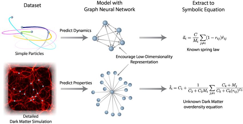
Discovering Symbolic Models from Deep Learning
                                                           with Inductive Biases

                                              Miles Cranmer1            Alvaro Sanchez-Gonzalez2             Peter Battaglia2        Rui Xu1

                                                       Kyle Cranmer3                 David Spergel4,1                Shirley Ho4,3,1,5
arXiv:2006.11287v2 [cs.LG] 18 Nov 2020

                                                            1                                           2
                                                              Princeton University, Princeton, USA        DeepMind, London, UK
                                                  3                                                4
                                                      New York University, New York City, USA        Flatiron Institute, New York City, USA
                                                                        5
                                                                          Carnegie Mellon University, Pittsburgh, USA

                                                                                         Abstract
                                                  We develop a general approach to distill symbolic representations of a learned
                                                  deep model by introducing strong inductive biases. We focus on Graph Neural
                                                  Networks (GNNs). The technique works as follows: we first encourage sparse
                                                  latent representations when we train a GNN in a supervised setting, then we
                                                  apply symbolic regression to components of the learned model to extract explicit
                                                  physical relations. We find the correct known equations, including force laws and
                                                  Hamiltonians, can be extracted from the neural network. We then apply our method
                                                  to a non-trivial cosmology example—a detailed dark matter simulation—and
                                                  discover a new analytic formula which can predict the concentration of dark matter
                                                  from the mass distribution of nearby cosmic structures. The symbolic expressions
                                                  extracted from the GNN using our technique also generalized to out-of-distribution-
                                                  data better than the GNN itself. Our approach offers alternative directions for
                                                  interpreting neural networks and discovering novel physical principles from the
                                                  representations they learn.

                                         1    Introduction
                                         The miracle of the appropriateness of the language of mathematics for the formulation of the laws of
                                         physics is a wonderful gift which we neither understand nor deserve. We should be grateful for it and
                                         hope that it will remain valid in future research and that it will extend, for better or for worse, to our
                                         pleasure, even though perhaps also to our bafflement, to wide branches of learning.—Eugene Wigner
                                         “The Unreasonable Effectiveness of Mathematics in the Natural Sciences” [1].
                                         For thousands of years, science has leveraged models made out of closed-form symbolic expressions,
                                         thanks to their many advantages: algebraic expressions are usually compact, present explicit inter-
                                         pretations, and generalize well. However, finding these algebraic expressions is difficult. Symbolic
                                         regression is one option: a supervised machine learning technique that assembles analytic functions
                                         to model a given dataset. However, typically one uses genetic algorithms—essentially a brute force
                                         procedure as in [2]—which scale exponentially with the number of input variables and operators.
                                         Many machine learning problems are thus intractable for traditional symbolic regression.
                                         On the other hand, deep learning methods allow efficient training of complex models on high-
                                         dimensional datasets. However, these learned models are black boxes, and difficult to interpret.
                                            Code for our models and experiments can be found at https://github.com/MilesCranmer/symbolic_
                                         deep_learning.

                                         34th Conference on Neural Information Processing Systems (NeurIPS 2020), Vancouver, Canada.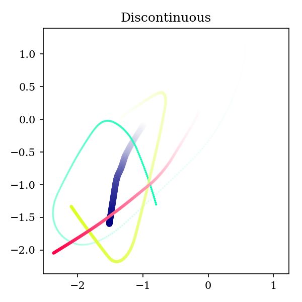
Figure 1: A cartoon depicting how we extract physical equations from a dataset.

Furthermore, generalization is difficult without prior knowledge about the data imposed directly on
the model. Even if we impose strong inductive biases on the models to improve generalization, the
learned parts of networks typically are linear piece-wise approximations which extrapolate linearly
(if using ReLU as activation [3]).
Here, we propose a general framework to leverage the advantages of both deep learning and symbolic
regression. As an example, we study Graph Networks (GNs or GNNs) [4] as they have strong and
well-motivated inductive biases that are very well suited to problems we are interested in. Then we
apply symbolic regression to fit different internal parts of the learned model that operate on reduced
size representations. The symbolic expressions can then be joined together, giving rise to an overall
algebraic equation equivalent to the trained GN. Our work is a generalized and extended version of
that in [5].
We apply our framework to three problems—rediscovering force laws, rediscovering Hamiltoni-
ans, and a real world astrophysical challenge—and demonstrate that we can drastically improve
generalization, and distill plausible analytical expressions. We not only recover the injected closed-
form physical laws for Newtonian and Hamiltonian examples, we also derive a new interpretable
closed-form analytical expression that can be useful in astrophysics.

2   Framework

Our framework can be summarized as follows. (1) Engineer a deep learning model with a separable
internal structure that provides an inductive bias well matched to the nature of the data. Specifically,
in the case of interacting particles, we use Graph Networks as the core inductive bias in our models.
(2) Train the model end-to-end using available data. (3) Fit symbolic expressions to the distinct
functions learned by the model internally. (4) Replace these functions in the deep model by the
symbolic expressions. This procedure with the potential to discover new symbolic expressions for
non-trivial datasets is illustrated in fig. 1.

Particle systems and Graph Networks. In this paper we focus on problems that can be well
described as interacting particle systems. Nearly all of the physics we experience in our day-to-day
life can be described in terms of interactions rules between particles or entities, so this is broadly
relevant. Recent work has leveraged the inductive biases of Interaction Networks (INs) [6] in their
generalized form, the Graph Network, a type of Graph Neural Network [7, 8, 9], to learn models of
particle systems in many physical domains [6, 10, 11, 12, 13, 14, 15, 16].
Therefore we use Graph Networks (GNs) at the core of our models, and incorporate into them
physically motivated inductive biases appropriate for each of our case studies. Some other interesting

                                                   2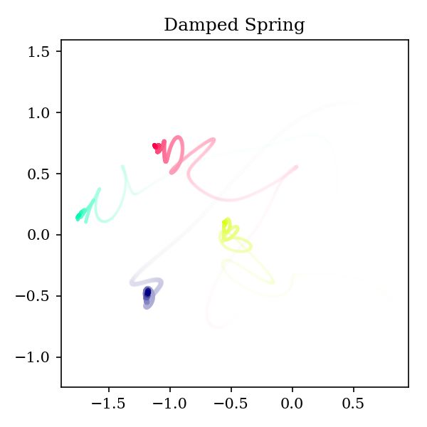
approaches for learning low-dimensional general dynamical models include [17, 18, 19]. Other
related work which studies the physical reasoning abilities of deep models include [20, 21, 22, 23].
Internally, GNs are structured into three distinct components: an edge model, a node model, and a
global model, which take on different but explicit roles in a regression problem. The edge model, or
“message function,” which we denote by φe , maps from a pair of nodes (vi , vj ∈ RLv ) connected by
an edge in a graph together with some vector information for the edge, to a message vector. These
message vectors are summed element-wise for each receiving node over all of their sending nodes,
and the summed vector is passed to the node model. The node model, φv , takes the receiving node
and the summed message vector, and computes an updated node: a vector representing some property
or dynamical update. Finally, a global model φu aggregates all messages and all updated nodes
and computes a global property. φe , φv , φu are usually approximated using multilayer-perceptrons,
making them differentiable end-to-end. More details on GNs are given in the appendix. We illustrate
the internal structure of a GN in fig. 2.

                                            Legend
                                         Data Vector

                                         Latent Vector
                                         Neural Network (MLP)                                Analogy to
                                                                  Graph Network          Newtonian Mechanics
             Input state
                                                                       Nodes                        Particles
                                                                    Pairs of nodes       Two interacting particles
                                                                  Edge model (       )        Compute force
           Encourage
            sparsity                                                Messages (   )
                                 +   +         +                        Pool               Sum into net force
                                                                Concatenate with node
                                                                  Node model (       )   Acceleration
                                                                   Updated nodes            Compute next timestep

                  Output state

                                                           Approximate with
                                                          symbolic regression

Figure 2: An illustration of the internal structure of the graph neural network we use in some of our
experiments. Note that the comparison to Newtonian mechanics is purely for explanatory purposes,
but is not explicit. Differences include: the “forces” (messages) are often high dimensional, the nodes
need not be physical particles, φe and φv are arbitrary learned functions, and the output need not be
an updated state. However, the rough equivalency between this architecture and physical frameworks
allows us to interpret learned formulas in terms of existing physics.

GNs are the ideal candidate for our approach due to their inductive biases shared by many physics
problems. (a) They are equivariant under particle permutations. (b) They are differentiable end-to-end
and can be trained efficiently using gradient descent. (c) They make use of three separate and
interpretable internal functions φe , φv , φu , which are our targets for the symbolic regression. GNs
can also be embedded with additional symmetries as in [24, 25], but we do not implement these.

Symbolic regression. After training the Graph Networks, we use the symbolic regression package
eureqa [2] to perform symbolic regression and fit compact closed-form analytical expressions to
φe , φv , and φu independently. eureqa works by using a genetic algorithm to combine algebraic
expressions stochastically. The technique is similar to natural selection, where the “fitness” of each
expression is defined in terms of simplicity and accuracy. The operators considered in the fitting
process are +, −, ×, /, >,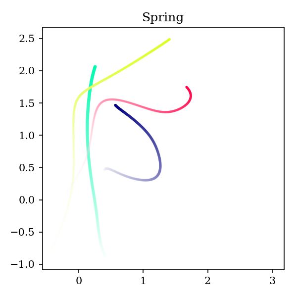
us to extend symbolic regression to high-dimensional datasets, where it is otherwise intractable. As
an example, consider attempting to discover the relationship between a scalar and a time series, given
data {(zi , {xi,1 , xi,2 , . . . xi,100 }}, where zi ∈ R and xi,j ∈ R5 . Assume the true relationship as
                     P100
zi = yi2 , for yi = j=1 yi,j , yi,j = exp xi,j,3 + cos 2xi,j,1 . Now, in a learnable model, assume
                                  P100
an inductive bias zi = f ( j=1 g(xi,j )) for scalar functions f and g. If we need to consider 109
equations for both f and g, then a standard symbolic regression search would need to consider their
combination, leading to (109 )2 = 1018 equations in total. But if we first fit a neural network for f and
g, and after training, fit an equation to f and g separately, we only need to consider 2 × 10⁹ equations.
In effect, we factorize high-dimensional datasets into smaller sub-problems that are tractable for
symbolic regression.
We emphasize that this method is not a new symbolic regression technique by itself; rather, it is a
way of extending any existing symbolic regression method to high-dimensional datasets by the use of
a neural network with a well-motivated inductive bias. While we chose eureqa for our experiments
based on its efficiency and ease-of-use, we could have chosen another low-dimensional symbolic
regression package, such as our new high-performance package PySR1 [27]. Other community pack-
ages such as [28, 29, 30, 31, 32, 33, 34, 35, 36], could likely also be used and achieve similar results
(although [32] is unable to fit the constants required for the tasks here). Ref. [29] is an interesting
approach that uses gradient descent on a pre-defined equation up to some depth, parametrized with a
neural network, instead of genetic algorithms; [35] uses gradient descent on a latent embedding of an
equation; and [36] demonstrates Monte Carlo Tree Search as a symbolic regression technique, using
an asymptotic constraint as input to a neural network which guides the search. These could all be
used as drop-in replacements for eureqa here to extend their algorithms to high-dimensional datasets.
We also note several exciting packages for symbolic regression of partial differential equations on
gridded data: [37, 38, 39, 40, 41, 42]. These either use sparse regression of coefficients over a
library of PDE terms, or a genetic algorithm. While not applicable to our use-cases, these would be
interesting to consider for future extensions to gridded PDE data.

Compact internal representations. While training, we encourage the model to use compact
internal representations for latent hidden features (e.g., messages) by adding regularization terms
to the loss (we investigate using L1 and KL penalty terms with a fixed prior, see more details in the
Appendix). One motivation for doing this is based on Occam’s Razor: science always prefers the
simpler model or representation of two which give similar accuracy. Another stronger motivation
is that if there is a law that perfectly describes a system in terms of summed message vectors in a
compact space (what we call a linear latent space), then we expect that a trained GN, with message
vectors of the same dimension as that latent space, will be mathematical rotations of the true vectors.
We give a mathematical explanation of this reasoning in the appendix, and emphasize that while it
may seem obvious now, our work is the first to demonstrate it. More practically, by reducing the size
of the latent representations, we can filter out all low-variance latent features without compromising
the accuracy of the model, and vastly reducing the dimensionality of the hidden vectors. This makes
the symbolic regression of the internal models more tractable.

Implementation details. We write our models with PyTorch [43] and PyTorch Geometric[44]. We
train them with a decaying learning schedule using Adam [45]. The symbolic regression technique is
described in section 4.1. More details are provided in the Appendix.

3       Case studies
In this section we present three specific case studies where we apply our proposed framework using
additional inductive biases.

Newtonian dynamics. Newtonian dynamics describes the dynamics of particles according to
Newton’s law of motion: the motion of each particle is modeled using incident forces from nearby
particles, which change its position, velocity and acceleration. Many important forces in physics
(e.g., gravitational force − Gmr12m2 r̂) are defined on pairs of particles, analogous to the message
function φe of our Graph Networks. The summation that aggregates messages is analogous to the
    1
        https://github.com/MilesCranmer/PySR

                                                   4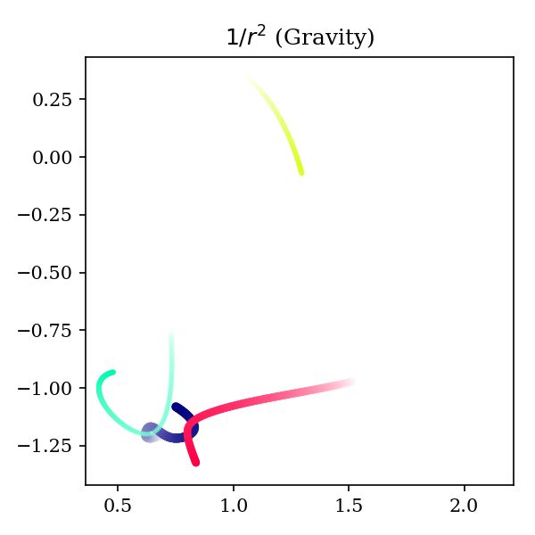
calculation of the net force on a receiving particle. Finally, the node function, φv , acts like Newton’s
law: acceleration equals the net force (the summed message) divided by the mass of the receiving
particle.
To train a model on Newtonian dynamics data, we train the GN to predict the instantaneous accelera-
tion of the particle against that calculated in the simulation. While Newtonian mechanics inspired the
original development of INs, never before has an attempt to distill the relationship between the forces
and the learned messages been successful. When applying the framework to this Newtonian dynamics
problem (as illustrated in fig. 1), we expect the model trained with our framework to discover that the
optimal dimensionality of messages should match the number of spatial dimensions. We also expect
to recover algebraic formulas for pairwise interactions, and generalize better than purely learned
models. We refer our readers to section 4.1 and the Appendix for more details.

Hamiltonian dynamics. Hamiltonian dynamics describes a system’s total energy H(q, p) as a
function of its canonical coordinates q and momenta p—e.g., each particle’s position and momentum.
The dynamics of the system change perpendicularly to the gradient of H: dq       ∂H dp      dH
                                                                           dt = ∂p , dt = − dq .

Here, we will use a variant of a Hamiltonian Graph Network (HGN) [46] to learn H for the Newtonian
dynamics data. This model is a combination of a Hamiltonian Neural Network [47, 48] and GN.
In this case, the global model φu of the GN will output a single scalar value for the entire system
representing the energy, and hence the GN will have the same functional form as a Hamiltonian. By
then taking the partial derivatives of the GN-predicted H with respect to the position and momentum,
q and p, respectively, of the input nodes, we will be able to calculate the updates to the momentum
and position. We impose a modification to the HGN to facilitate its interpretability, and name this the
“Flattened HGN” or FlatHGN: instead of summing high-dimensional encodings of nodes to calculate
φu , we instead set it to be a sum of scalar pairwise interaction terms, Hpair and a per-particle term,
Hself . This is because many physical systems can be exactly described this way. This is a Hamiltonian
version of the Lagrangian Graph Network in [49], and is similar to [50]. This is still general enough
to express many physical systems, as nearly all of physics can be written as summed interaction
energies, but could also be relaxed in the context of the framework.
Even though the model is trained end-to-end, we expect our framework to allow us to extract analytical
expressions for both the per-particle kinetic energy, and the scalar pairwise potential energy. We refer
our readers to our section 4.2 and the Appendix for more details.

Dark matter halos for cosmology. We also apply our framework to a dataset generated from state-
of-the-art dark matter simulations [51]. We predict a property (“overdensity”) of a dark matter blob
(called a “halo”) from the properties (positions, velocities, masses) of halos nearby. We would like to
extract this relationship as an analytic expression so we may interpret it theoretically. This problem
differs from the previous two use cases in many ways, including (1) it is a real-world problem where
an exact analytical expression is unknown; (2) the problem does not involve dynamics, rather, it is a
regression problem on a static dataset; and (3) the dataset is not made of particles, but rather a grid
of density that has been grouped and reduced to handmade features. Similarly, we do not know the
dimensionality of interactions, should a linear latent space exist. We rely on our inductive bias to find
the optimal dimensional of the problem, and then yield an interpretable model that performs better
than existing analytical approximations. We refer our readers to our section 4.3 and the Appendix for
further details.

4     Experiments & results
4.1   Newtonian dynamics

We train our Newtonian dynamics GNs on data for simple N-body systems with known force laws.
We then apply our technique to recover the known force laws via the representations learned by the
message function φe .

Data. The dataset consists of N-body particle simulations in two and three dimensions, under
different interaction laws. We used the following forces: (a) 1/r orbital force: −m1 m2 r̂/r; (b) 1/r2
                                                                                                      2
orbital force −m1 m2 r̂/r2 ; (c) charged particles force q1 q2 r̂/r2 ; (d) damped springs with |r − 1|

                                                   5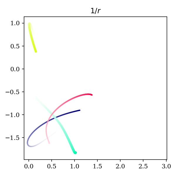
Dataset                                       Graph Network:

                                                      Make Prediction,
                                                        Compare,
                                                      Update Weights

                                                                             Record
                                                                             Messages

                                        Apply L
                                     Regularization                        Sorted by largest standard deviation

  Validate by fitting to                                                          Alternatively, use symbolic
      known force:                                                                   regression to extract
                                                                                        unknown force:

                                                                                which we can see is a rotation of the
                                                                                            true force:

                                                                                    Force = −(r − 1)r̂

Figure 3: A diagram showing how we implement and exploit our inductive bias on GNs. A video of
this figure during training can be seen by going to the URL https://github.com/MilesCranmer/
symbolic_deep_learning/blob/master/video_link.txt.

potential and damping proportional and opposite to speed; (e) discontinuous forces, −{0, r2 }r̂,
switching to 0 force for r < 2; and (f) springs between all particles, a (r − 1)2 potential. The
simulations themselves contain masses and charges of 4 or 8 particles, with positions, velocities, and
accelerations as a function of time. Further details of these systems are given in the appendix, with
example trajectories shown in fig. 4.

Model training. The models are trained to predict instantaneous acceleration for every particle
given the current state of the system. To investigate the importance of the size of the message
representations for interpreting the messages as forces, we train our GN using 4 different strategies:
1. Standard, a GN with 100 message components; 2. Bottleneck, a GN with the number of message
components matching the dimensionality of the problem (2 or 3); 3. L1 , same as “Standard” but using
a L1 regularization loss term on the messages with a weight of 10−2 ; and 4. KL same as “Standard”
but regularizing the messages using the Kullback-Leibler (KL) divergence with respect to Gaussian
prior. Both the L1 and KL strategies encourage the network to find compact representations for the
message vectors, using different regularizations. We optimize the mean absolute loss between the
predicted acceleration and the true acceleration of each node. Additional training details are given in
the appendix and found in the codebase.

Performance comparison. To evaluate the learned models, we generate a new dataset from a
different random seed. We find that the model with L1 regularization has the greatest prediction
performance in most cases (see table 3). It is worth noting that the bottleneck model, even though it
has the correct dimensionalty, performs worse than the model using L1 regularization under limited
training time. We speculate that this may connect to the lottery ticket hypothesis [52].

Interpreting the message components. As a first attempt to interpret the information in the
message components, we pick the D message features (where D is the dimensionality of the
simulation) with the highest variance (or KL divergence), and fit each to a linear combination of the
true force components. We find that while the GN trained in the Standard setting does not show strong

                                                               6
correlations with force components (also seen in fig. 5), all other models for which the effective
message size is constrained explicitly (bottleneck) or implicitly (KL or L1 ) to be low dimensional
yield messages that are highly correlated with the true forces (see table 1 which indicates the fit errors
with respect to the true forces), with the model trained with L1 regularization showing the highest
correlations. An explicit demonstration that the messages in a graph network learn forces has not
been observed before our work.
The messages in these models are thus explicitly interpretable as forces. The video
at https://github.com/MilesCranmer/symbolic_deep_learning/blob/master/video_
link.txt (fig. 3) shows a fit of the message components over time during training, showing how the
model discovers a message representation that is highly correlated with a rotation of the true force
vector in an unsupervised way.
Sim. Standard Bottleneck L1 KL
Charge-2 0.016 0.947 0.004 0.185
Charge-3 0.013 0.980 0.002 0.425
r−1 -2 0.000 1.000 1.000 0.796
r−1 -3 0.000 1.000 1.000 0.332
r−2 -2 0.004 0.993 0.990 0.770
r−2 -3 0.002 0.994 0.977 0.214
Spring-2 0.032 1.000 1.000 0.883
Spring-3 0.036 0.995 1.000 0.214
Table 1: The R2 value of a fit of a linear combination of true force components to the message
components for a given model (see text). Numbers close to 1 indicate the messages and true force are
strongly correlated. Successes/failures of force law symbolic regression are tabled in the appendix.
Symbolic regression on the internal functions. We now demonstrate symbolic regression to
extract force laws from the messages, without using prior knowledge for each force’s form. To do
this, we record the most significant message component of φe , which we refer to as φe1 , over random
samples of the training dataset. The inputs to the regression are m1 , m2 , q1 , q2 , x1 , x2 , . . . (mass,
charge, x-position of receiving and sending node) as well as simplified variables to help the symbolic
regression: e.g., ∆x for x displacement, and r for distance.
We then use eureqa to fit the φe1 to the inputs by minimizing the mean absolute error (MAE) over
various analytic functions. Analogous to Occam’s razor, we find the “best” algebraic model by asking
eureqa to provide multiple candidate fits at different complexity levels (where complexity is scored as
a function of the number and the type of operators, constants and input variables used), and select the
fit that maximizes the fractional drop in mean absolute error (MAE) over the increase in complexity
from the next best model: (−∆ log(MAEc )/∆c). From this, we recover many analytical expressions
(this is tabled in the appendix) that are equivalent to the simulated force laws (a, b indicate learned
constants):
• Spring, 2D, L1 (expect φe1 ≈ (a · (∆x, ∆y))(r − 1) + b).
0.60∆x + 1.37∆y
φe1 ≈ 1.36∆y + 0.60∆x − − 0.0025
r
a·(∆x,∆y,∆z)
• 1/r2 , 3D, Bottleneck (expect φe1 ≈ r3 + b).
0.021∆xm2 − 0.077∆ym2
φe1 ≈
r3
• Discontinuous, 2D, L1 (expect φe1 ≈ IF(r > 2, (a · (∆x, ∆y, ∆z))r, 0) + b).
φe1 ≈ IF(r > 2, 0.15r∆y + 0.19r∆x, 0) − 0.038
Note that reconstruction does not always succeed, especially for training strategies other than L1 or
bottleneck models that cannot successfully find compact representations of the right dimensionality
(see some examples in Appendix).
74.2 Hamiltonian dynamics
Using the same datasets from the Newtonian dynamics case study, we also train our “FlatHGN,” with
the Hamiltonian inductive bias, and demonstrate that we can extract scalar potential energies, rather
than forces, for all of our problems. For example, in the case of charged particles, with expected
potential (Hpair ≈ aqr1 q2 ), symbolic regression applied to the learned message function yields2 :
Hpair ≈ 0.0019q
r
1 q2
.
It is also possible to fit the per-particle term Hself , however, in this case the same kinetic energy
expression is recovered for all systems. In terms of performance results, the Hamiltonian models are
comparable to that of the L1 regularized model across all datasets (See Supplementary results table).
Note that in this case, by design, the “FlatHGN“ has a message function with a dimensionality of 1 to
match the output of the Hamiltonian function which is a scalar, so no regularization is needed, as the
message size is directly constrained to the right dimension.
4.3 Dark matter halos for cosmology
Now, one may ask: “will this strategy also work for general regression problems, non-trivial datasets,
complex interactions, and unknown laws?” Here we give an example that satisfies all four of these
concerns, using data from a gravitational simulation of the Universe.
Cosmology studies the evolution of the Universe from the Big Bang to the complex galaxies and
stars we see today [53]. The interactions of various types of matter and energy drive this evolution.
Dark Matter alone consists of ≈ 85% of the total matter in the Universe [54, 55], and therefore is
extremely important for the development of galaxies. Dark matter particles clump together and act as
gravitational basins called “halos” which pull regular baryonic matter together to produce stars, and
form larger structures such as filaments and galaxies. It is an important question in cosmology to
predict properties of dark matter halos based on their “environment,” which consist of other nearby
dark matter halos. Here we study the following problem: how can we predict the excess amount of
matter (in comparison to its surroundings, δ = ρ−hρi
hρi ) for a dark matter halo based on its properties
and those of its neighboring dark matter halos?
A hand-designed estimator for the functional form of δi for halo i might correlate δ with the mass of
the same halo, Mi , as well as the mass within 20 distance units (we decide to use 20 as the smoothing
P|ri −rj |D E
Test Formula Summed Component |δi −δ̂i |
Constant δ̂i = C1 N/A 0.421
Old
P|ri −rj | 1.
We then proceed through the same training procedure as before, learning a GN to predict δ with L1
regularization, and then extracting messages for examples in the training set. Remarkably, we obtain
a functionally identical expression when extracting the formula from the graph network on this subset
of the data. We fit these constants to the same masked portion of data on which the graph network
was trained. The graph network itself obtains an average error h|δi − δ̂i | i = 0.0634 on the training
set, and 0.142 on the out-of-distribution data. Meanwhile, the symbolic expression achieves 0.0811
on the training set, but 0.0892 on the out-of-distribution data. Therefore, for this problem, it seems
a symbolic expression generalizes much better than the very graph neural network it was extracted
from. This alludes back to Eugene Wigner’s article: the language of simple, symbolic models is
remarkably effective in describing the universe.
5 Conclusion
We have demonstrated a general approach for imposing physically motivated inductive biases on
GNs and Hamiltonian GNs to learn interpretable representations, and potentially improved zero-shot
generalization. Through experiment, we have shown that GN models which implement a bottleneck
or L1 regularization in the message passing layer, or a Hamiltonian GN flattened to pairwise and
self-terms, can learn message representations equivalent to linear transformations of the true force
vector or energy. We have also demonstrated a generic technique for finding an unknown force
law from these models: symbolic regression is capable of fitting explicit equations to our trained
model’s message function. We repeated this for energies instead of forces via introduction of the
“Flattened Hamiltonian Graph Network.” Because GNs have more explicit substructure than their
more homogeneous deep learning relatives (e.g., plain MLPs, convolutional networks), we can draw
more fine-grained interpretations of their learned representations and computations. Finally, we have
demonstrated our algorithm on a non-trivial dataset, and discovered a new law for cosmological dark
matter.
9Acknowledgments and Disclosure of Funding
Miles Cranmer would like to thank Christina Kreisch and Francisco Villaescusa-Navarro for assistance
with the cosmology dataset; and Christina Kreisch, Oliver Philcox, and Edgar Minasyan for comments
on a draft of the paper. The authors would like to thank the reviewers for insightful feedback that
improved this paper. Shirley Ho and David Spergel’s work is supported by the Simons Foundation.
Our code made use of the following Python packages: numpy, scipy, sklearn, jupyter,
matplotlib, pandas, torch, tensorflow, jax, and torch_geometric [58, 59, 60, 61, 62, 63,
43, 64, 65, 44].
References
[1] Eugene P. Wigner. The unreasonable effectiveness of mathematics in the natural sci-
ences. Communications on Pure and Applied Mathematics, 13(1):1–14, 1960. doi: 10.
1002/cpa.3160130102. URL https://onlinelibrary.wiley.com/doi/abs/10.1002/
cpa.3160130102.
[2] Michael Schmidt and Hod Lipson. Distilling free-form natural laws from experimental data.
science, 324(5923):81–85, 2009.
[3] Guido F Montufar, Razvan Pascanu, Kyunghyun Cho, and Yoshua Bengio. On the number of
linear regions of deep neural networks. In Advances in neural information processing systems,
pages 2924–2932, 2014.
[4] Peter W Battaglia, Jessica B Hamrick, Victor Bapst, Alvaro Sanchez-Gonzalez, Vinicius
Zambaldi, Mateusz Malinowski, Andrea Tacchetti, David Raposo, Adam Santoro, Ryan
Faulkner, et al. Relational inductive biases, deep learning, and graph networks. arXiv preprint
arXiv:1806.01261, 2018.
[5] Miles D Cranmer, Rui Xu, Peter Battaglia, and Shirley Ho. Learning Symbolic Physics with
Graph Networks. arXiv preprint arXiv:1909.05862, 2019.
[6] Peter Battaglia, Razvan Pascanu, Matthew Lai, Danilo Jimenez Rezende, et al. Interaction
networks for learning about objects, relations and physics. In Advances in neural information
processing systems, pages 4502–4510, 2016.
[7] Franco Scarselli, Marco Gori, Ah Chung Tsoi, Markus Hagenbuchner, and Gabriele Monfardini.
The graph neural network model. IEEE Transactions on Neural Networks, 20(1):61–80, 2009.
[8] Michael M Bronstein, Joan Bruna, Yann LeCun, Arthur Szlam, and Pierre Vandergheynst.
Geometric deep learning: going beyond euclidean data. IEEE Signal Processing Magazine, 34
(4):18–42, 2017.
[9] Justin Gilmer, Samuel S Schoenholz, Patrick F Riley, Oriol Vinyals, and George E Dahl. Neural
message passing for quantum chemistry. In Proceedings of the 34th International Conference
on Machine Learning-Volume 70, pages 1263–1272. JMLR. org, 2017.
[10] Michael B Chang, Tomer Ullman, Antonio Torralba, and Joshua B Tenenbaum. A compositional
object-based approach to learning physical dynamics. arXiv preprint arXiv:1612.00341, 2016.
[11] Alvaro Sanchez-Gonzalez, Nicolas Heess, Jost Tobias Springenberg, Josh Merel, Martin Ried-
miller, Raia Hadsell, and Peter Battaglia. Graph networks as learnable physics engines for
inference and control. arXiv preprint arXiv:1806.01242, 2018.
[12] Damian Mrowca, Chengxu Zhuang, Elias Wang, Nick Haber, Li F Fei-Fei, Josh Tenenbaum,
and Daniel L Yamins. Flexible neural representation for physics prediction. In Advances in
Neural Information Processing Systems, pages 8799–8810, 2018.
[13] Yunzhu Li, Jiajun Wu, Russ Tedrake, Joshua B Tenenbaum, and Antonio Torralba. Learning
particle dynamics for manipulating rigid bodies, deformable objects, and fluids. arXiv preprint
arXiv:1810.01566, 2018.
10[14] Thomas Kipf, Ethan Fetaya, Kuan-Chieh Wang, Max Welling, and Richard Zemel. Neural
relational inference for interacting systems. arXiv preprint arXiv:1802.04687, 2018.
[15] Victor Bapst, Thomas Keck, A Grabska-Barwińska, Craig Donner, Ekin Dogus Cubuk,
SS Schoenholz, Annette Obika, AWR Nelson, Trevor Back, Demis Hassabis, et al. Unveiling
the predictive power of static structure in glassy systems. Nature Physics, 16(4):448–454, 2020.
[16] Alvaro Sanchez-Gonzalez, Jonathan Godwin, Tobias Pfaff, Rex Ying, Jure Leskovec, and
Peter W Battaglia. Learning to simulate complex physics with graph networks. arXiv preprint
arXiv:2002.09405, 2020.
[17] Norman H Packard, James P Crutchfield, J Doyne Farmer, and Robert S Shaw. Geometry from
a time series. Physical review letters, 45(9):712, 1980.
[18] Bryan C. Daniels and Ilya Nemenman. Automated adaptive inference of phenomenological
dynamical models. Nature Communications, 6(1):1–8, August 2015. ISSN 2041-1723.
[19] Miguel Jaques, Michael Burke, and Timothy Hospedales. Physics-as-Inverse-Graphics: Joint
Unsupervised Learning of Objects and Physics from Video. arXiv:1905.11169 [cs], May 2019.
[20] Michael Janner, Sergey Levine, William T. Freeman, Joshua B. Tenenbaum, Chelsea Finn, and
Jiajun Wu. Reasoning About Physical Interactions with Object-Centric Models. In International
Conference on Learning Representations, 2019. URL https://openreview.net/forum?
id=HJx9EhC9tQ.
[21] Anton Bakhtin, Laurens van der Maaten, Justin Johnson, Laura Gustafson, and Ross Girshick.
PHYRE: A New Benchmark for Physical Reasoning. In H. Wallach, H. Larochelle, A. Beygelz-
imer, F. d'Alché-Buc, E. Fox, and R. Garnett, editors, Advances in Neural Information Process-
ing Systems 32, pages 5082–5093. Curran Associates, Inc., 2019. URL http://papers.nips.
cc/paper/8752-phyre-a-new-benchmark-for-physical-reasoning.pdf.
[22] Keyulu Xu, Jingling Li, Mozhi Zhang, Simon S. Du, Ken ichi Kawarabayashi, and Stefanie
Jegelka. What Can Neural Networks Reason About? In International Conference on Learning
Representations, 2020. URL https://openreview.net/forum?id=rJxbJeHFPS.
[23] Samuel S Schoenholz, Ekin D Cubuk, Daniel M Sussman, Efthimios Kaxiras, and Andrea J Liu.
A structural approach to relaxation in glassy liquids. Nature Physics, 12(5):469–471, 2016.
[24] Erik J Bekkers. B-Spline CNNs on Lie Groups. 2019.
[25] Marc Finzi, Samuel Stanton, Pavel Izmailov, and Andrew Gordon Wilson. Generalizing
Convolutional Neural Networks for Equivariance to Lie Groups on Arbitrary Continuous Data.
2020.
[26] Rex Ying, Dylan Bourgeois, Jiaxuan You, Marinka Zitnik, and Jure Leskovec. GNN Explainer:
A tool for post-hoc explanation of graph neural networks. arXiv preprint arXiv:1903.03894,
2019.
[27] Miles Cranmer. PySR: Fast & Parallelized Symbolic Regression in Python/Julia, September
2020. URL https://doi.org/10.5281/zenodo.4052869.
[28] Dario Izzo and Francesco Biscani. dcgp: Differentiable Cartesian Genetic Programming made
easy., May 2020. URL https://doi.org/10.5281/zenodo.3802555.
[29] Subham Sahoo, Christoph Lampert, and Georg Martius. Learning Equations for Extrapolation
and Control. volume 80 of Proceedings of Machine Learning Research, pages 4442–4450,
Stockholmsmässan, Stockholm Sweden, 10–15 Jul 2018. PMLR. URL http://proceedings.
mlr.press/v80/sahoo18a.html.
[30] Georg Martius and Christoph H. Lampert. Extrapolation and learning equations, 2016.
[31] Félix-Antoine Fortin, François-Michel De Rainville, Marc-André Gardner, Marc Parizeau, and
Christian Gagné. DEAP: Evolutionary algorithms made easy. Journal of Machine Learning
Research, 13(70):2171–2175, 2012.
11[32] Silviu-Marian Udrescu and Max Tegmark. AI Feynman: A physics-inspired method for
symbolic regression. Science Advances, 6(16):eaay2631, 2020.
[33] Tony Worm and Kenneth Chiu. Prioritized Grammar Enumeration: Symbolic Regression by
Dynamic Programming. In Proceedings of the 15th Annual Conference on Genetic and Evolu-
tionary Computation, GECCO ’13, page 1021–1028, New York, NY, USA, 2013. Association
for Computing Machinery. ISBN 9781450319638. doi: 10.1145/2463372.2463486. URL
https://doi.org/10.1145/2463372.2463486.
[34] Roger Guimerà, Ignasi Reichardt, Antoni Aguilar-Mogas, Francesco A. Massucci, Manuel
Miranda, Jordi Pallarès, and Marta Sales-Pardo. A Bayesian machine scientist to aid in the
solution of challenging scientific problems. Science Advances, 6(5), 2020. doi: 10.1126/sciadv.
aav6971. URL https://advances.sciencemag.org/content/6/5/eaav6971.
[35] Matt J. Kusner, Brooks Paige, and José Miguel Hernández-Lobato. Grammar Variational
Autoencoder, 2017.
[36] Li Li, Minjie Fan, Rishabh Singh, and Patrick Riley. Neural-guided symbolic regression with
asymptotic constraints. arXiv preprint arXiv:1901.07714, 2019.
[37] Gert-Jan Both, Subham Choudhury, Pierre Sens, and Remy Kusters. DeepMoD: Deep learning
for Model Discovery in noisy data, 2019.
[38] Steven L Brunton, Joshua L Proctor, and J Nathan Kutz. Discovering governing equations
from data by sparse identification of nonlinear dynamical systems. Proceedings of the national
academy of sciences, 113(15):3932–3937, 2016.
[39] Steven Atkinson, Waad Subber, Liping Wang, Genghis Khan, Philippe Hawi, and Roger
Ghanem. Data-driven discovery of free-form governing differential equations. arXiv preprint
arXiv:1910.05117, 2019.
[40] Christopher Rackauckas, Yingbo Ma, Julius Martensen, Collin Warner, Kirill Zubov, Rohit
Supekar, Dominic Skinner, and Ali Ramadhan. Universal differential equations for scientific
machine learning. arXiv preprint arXiv:2001.04385, 2020.
[41] Zhao Chen, Yang Liu, and Hao Sun. Deep learning of physical laws from scarce data, 2020.
[42] Harsha Vaddireddy, Adil Rasheed, Anne E. Staples, and Omer San. Feature engineering and
symbolic regression methods for detecting hidden physics from sparse sensor observation data.
Physics of Fluids, 32(1):015113, 2020. doi: 10.1063/1.5136351. URL https://doi.org/10.
1063/1.5136351.
[43] Adam Paszke, Sam Gross, Francisco Massa, Adam Lerer, James Bradbury, Gregory Chanan,
Trevor Killeen, Zeming Lin, Natalia Gimelshein, Luca Antiga, Alban Desmaison, Andreas
Kopf, Edward Yang, Zachary DeVito, Martin Raison, Alykhan Tejani, Sasank Chilamkurthy,
Benoit Steiner, Lu Fang, Junjie Bai, and Soumith Chintala. PyTorch: An Imperative Style, High-
Performance Deep Learning Library. In H. Wallach, H. Larochelle, A. Beygelzimer, F. d'Alché-
Buc, E. Fox, and R. Garnett, editors, Advances in Neural Information Processing Systems 32,
pages 8024–8035. Curran Associates, Inc., 2019. URL http://papers.neurips.cc/paper/
9015-pytorch-an-imperative-style-high-performance-deep-learning-library.
pdf.
[44] Matthias Fey and Jan E. Lenssen. Fast Graph Representation Learning with PyTorch Geometric.
In ICLR Workshop on Representation Learning on Graphs and Manifolds, 2019.
[45] Diederik P Kingma and J Adam Ba. A method for stochastic optimization. arXiv preprint
arXiv:1412.6980, 2014.
[46] Alvaro Sanchez-Gonzalez, Victor Bapst, Kyle Cranmer, and Peter Battaglia. Hamiltonian graph
networks with ode integrators. arXiv preprint arXiv:1909.12790, 2019.
[47] Samuel Greydanus, Misko Dzamba, and Jason Yosinski. Hamiltonian neural networks. In
Advances in Neural Information Processing Systems, pages 15353–15363, 2019.
12[48] Peter Toth, Danilo Jimenez Rezende, Andrew Jaegle, Sébastien Racanière, Aleksandar Botev,
and Irina Higgins. Hamiltonian generative networks. arXiv preprint arXiv:1909.13789, 2019.
[49] Miles Cranmer, Sam Greydanus, Stephan Hoyer, Peter Battaglia, David Spergel, and Shirley Ho.
Lagrangian Neural Networks. In ICLR 2020 Workshop on Integration of Deep Neural Models
and Differential Equations, 2020.
[50] Jiang Wang, Simon Olsson, Christoph Wehmeyer, Adrià Pérez, Nicholas E Charron, Gianni
De Fabritiis, Frank Noé, and Cecilia Clementi. Machine learning of coarse-grained molecular
dynamics force fields. ACS central science, 5(5):755–767, 2019.
[51] Francisco Villaescusa-Navarro, ChangHoon Hahn, Elena Massara, Arka Banerjee, Ana Maria
Delgado, Doogesh Kodi Ramanah, Tom Charnock, Elena Giusarma, Yin Li, Erwan Allys, et al.
The Quijote simulations. arXiv preprint arXiv:1909.05273, 2019.
[52] Jonathan Frankle and Michael Carbin. The lottery ticket hypothesis: Finding sparse, trainable
neural networks. In International Conference on Learning Representations, 2018.
[53] Scott Dodelson. Modern cosmology. 2003.
[54] David N Spergel, Licia Verde, Hiranya V Peiris, E Komatsu, MR Nolta, CL Bennett, M Halpern,
G Hinshaw, N Jarosik, A Kogut, et al. First-year Wilkinson Microwave Anisotropy Probe
(WMAP)* observations: determination of cosmological parameters. The Astrophysical Journal
Supplement Series, 148(1):175, 2003.
[55] Planck Collaboration. Planck 2018 results. VI. Cosmological parameters. arXiv e-prints, art.
arXiv:1807.06209, July 2018.
[56] Carlos S. Frenk, Simon D. M. White, Marc Davis, and George Efstathiou. The Formation of
Dark Halos in a Universe Dominated by Cold Dark Matter. Astrophysical Journal, 327:507,
April 1988. doi: 10.1086/166213.
[57] Gary Marcus. The next decade in AI: four steps towards robust artificial intelligence. arXiv
preprint arXiv:2002.06177, 2020.
[58] S. van der Walt, S. C. Colbert, and G. Varoquaux. The NumPy Array: A Structure for Efficient
Numerical Computation. Computing in Science Engineering, 13(2):22–30, 2011.
[59] Pauli Virtanen, Ralf Gommers, Travis E. Oliphant, Matt Haberland, Tyler Reddy, David
Cournapeau, Evgeni Burovski, Pearu Peterson, Warren Weckesser, Jonathan Bright, Stéfan J.
van der Walt, Matthew Brett, Joshua Wilson, K. Jarrod Millman, Nikolay Mayorov, Andrew
R. J. Nelson, Eric Jones, Robert Kern, Eric Larson, CJ Carey, İlhan Polat, Yu Feng, Eric W.
Moore, Jake Vand erPlas, Denis Laxalde, Josef Perktold, Robert Cimrman, Ian Henriksen,
E. A. Quintero, Charles R Harris, Anne M. Archibald, Antônio H. Ribeiro, Fabian Pedregosa,
Paul van Mulbregt, and SciPy 1. 0 Contributors. SciPy 1.0: Fundamental Algorithms for
Scientific Computing in Python. Nature Methods, 17:261–272, 2020. doi: https://doi.org/10.
1038/s41592-019-0686-2.
[60] Fabian Pedregosa, Gaël Varoquaux, Alexandre Gramfort, Vincent Michel, Bertrand Thirion,
Olivier Grisel, Mathieu Blondel, Peter Prettenhofer, Ron Weiss, Vincent Dubourg, Jake Vander-
plas, Alexandre Passos, David Cournapeau, Matthieu Brucher, Matthieu Perrot, and Édouard
Duchesnay. Scikit-learn: Machine Learning in Python. Journal of Machine Learning Research,
12(85):2825–2830, 2011. URL http://jmlr.org/papers/v12/pedregosa11a.html.
[61] Thomas Kluyver, Benjamin Ragan-Kelley, Fernando Pérez, Brian Granger, Matthias Bussonnier,
Jonathan Frederic, Kyle Kelley, Jessica Hamrick, Jason Grout, Sylvain Corlay, Paul Ivanov,
Damián Avila, Safia Abdalla, and Carol Willing. Jupyter Notebooks – a publishing format for
reproducible computational workflows. In F. Loizides and B. Schmidt, editors, Positioning and
Power in Academic Publishing: Players, Agents and Agendas, pages 87 – 90. IOS Press, 2016.
[62] J. D. Hunter. Matplotlib: A 2D Graphics Environment. Computing in Science & Engineering, 9
(3):90–95, 2007.
13[63] Wes McKinney. Data Structures for Statistical Computing in Python. In Stéfan van der Walt
and Jarrod Millman, editors, Proceedings of the 9th Python in Science Conference, pages 56 –
61, 2010. doi: 10.25080/Majora-92bf1922-00a.
[64] Martín Abadi, Paul Barham, Jianmin Chen, Zhifeng Chen, Andy Davis, Jeffrey Dean, Matthieu
Devin, Sanjay Ghemawat, Geoffrey Irving, Michael Isard, et al. Tensorflow: A system for
large-scale machine learning. In 12th {USENIX} Symposium on Operating Systems Design and
Implementation ({OSDI} 16), pages 265–283, 2016.
[65] James Bradbury, Roy Frostig, Peter Hawkins, Matthew James Johnson, Chris Leary, Dougal
Maclaurin, and Skye Wanderman-Milne. JAX: composable transformations of Python+NumPy
programs, 2018. URL http://github.com/google/jax.
14Supplementary
A Model Implementation Details
Code for our implementation can be found at https://github.com/MilesCranmer/symbolic_
deep_learning. Here we describe how one can implement our model from scratch in a deep
learning framework. The main argument in this paper is that one can apply strong inductive biases to
a deep learning model to simplify the extraction of a symbolic representation of the learned model.
While we emphasize that this idea is general, in this section we focus on the specific Graph Neural
Networks we have used as an example throughout the paper.
A.1 Basic Graph Representation
We would like to use the graph G = (V, E) to predict an updated graph G0 = (V 0 , E). Our input
dataset is a graph G = (V, E) consisting of N v nodes with Lv features each: V = {vi }i=1:N v ,
v
with each vi ∈ RL . The nodes are connected by N e edges: E = {(rk , sk )}k=1:N e , where
rk , sk ∈ {1 : N v } are the indices for the receiving and sending nodes, respectively. We would like
v0
to use this graph to predict another graph V 0 = {vi0 }i=1:N v , where each vi0 ∈ RL is the node
corresponding to vi . The number of features in these predicted nodes, Lv0 , need not necessarily be
the same as for the input nodes (Lv ), though this could be the case for dynamical models where one
is predicting updated states of particles. For more general regression problems, the number of output
features is arbitrary.
Edge model. The prediction is done in two parts. We create the first neural network, the edge model
v v e0
(or “message function”), to compute messages from one node to another: φe : RL × RL → RL .
0 0
Here, Le is the number of message features. In the bottleneck model, one sets Le equal to the known
0
dimension of the force, which is 2 or 3 for us. In our models, we set Le = 100 for the standard and
L1 models, and 200 for the KL model (which is described separately later on). We create φe as a
multi-layer perceptron with ReLU activations and two hidden layers, each with 300 hidden nodes.
The mapping is e0k = φe (vrk , vsk ) for all edges indexed by k (i.e., we concatenate the receiving and
sending node features).
Aggregation. These messages are then pooled via element-wise summation for each receiving
e0
node i into the summed message, ē0i ∈ RL . This can be written as ē0i = k∈{1:N e |rk =i} e0k .
P
Node model. We create a second neural network to predict the output nodes, vi0 , for each i from the
v e0 v0
corresponding summed message and input node. This net can be written as φv : RL × RL → RL ,
and has the mapping: v̂i0 = φv (vi , ē0i ), where v̂i0 is the prediction for vi0 . We also create φv as a
15multi-layer perceptron with ReLU activations and two hidden layers, each with 300 hidden nodes.
This model is then trained with the loss function as described later in this section.
Summary. We can write out our forward model for the bottleneck, standard, and L1 models as:
Input graph G = (V, E) with
v
nodes (e.g., positions of particles) V = {vi }i=1:N v ; vi ∈ RL , and
edges (indices of connected nodes) E = {(rk , sk )}k=1:N e ; rk , sk ∈ {1 : N v }.
Compute messages for each edge: e0k = φe (vrk , vsk ),
e0
e0k ∈ RL , then
X
sum for each receiving node i : ē0i = e0k ,
k∈{1:N e |r k =i}
0
Le
ē0i ∈R .
Compute output node prediction: v̂i0 = φv (vi , ē0i )
v0
v̂i0 ∈ RL .
Loss. We jointly optimize the parameters in φv and φe via mini-batch gradient descent with Adam
as the optimizer. Our total loss function for optimizing is:
L = Lv + α1 Le + α2 Ln , where
1 X
the prediction loss is Lv = v vi0 − v̂i0 ,
N v
i∈{1:N }
P
0
1 k∈{1:N e } ek , L1
the message regularization is Le = e 0, Standard ,
N 0, Bottleneck
with the regularization constant α1 = 10−2 , and the
X 2
regularization for the network weights is Ln = |wl | ,
l={1:N l }
with α2 = 10−8 ,
where vi0 is the true value for the predicted node i. wl is the l-th network parameter out
of N l total parameters. This implementation can be visualized during training in the video
https://github.com/MilesCranmer/symbolic_deep_learning. During training, we also ap-
ply a random translation augmentation to all the particle positions to artificially generate more training
data.
Next, we describe the KL variant of this model. Note that for the cosmology example in section 4.3,
we use the L1 model described above with 500 hidden nodes (found with coarse hyperparameter
tuning to optimize accuracy) instead of 300, but other parameters are set the same.
A.2 KL Model
The KL model is a variational version of the GN implementation above, which models the messages
as distributions. We choose a normal distribution for each message component with a prior of
µ = 0, σ = 1. More specifically, the output of φe should now map to twice as many features as it
0
is predicting a mean and variance, hence we set Le = 200. The first half of the outputs of φe now
represent the means, and the second half of the outputs represent the log variance of a particular
16message component. In other words,
µ0k = φe1:100 (vrk , vsk ),
σ 02 e
k = exp φ101:200 (vrk , vsk ) ,
e0k ∼ N (µ0k , diag(σ 02
k )),
X
ē0i = e0k ,
k∈{1:N e |rk =i}
v̂i0
= φv (vi , ē0i ),
where N is a multinomial Gaussian distribution. Every time the graph network is run, we calculate
the mean and log variance of messages, sample each message once to calculate e0k , and pass those
samples through a sum to compute a sample of ē0i and then pass that value through the edge function
to compute a sample of v̂i0 . The loss is calculated normally, except for Le , which becomes the KL
divergence with respect to our Gaussian prior of µ = 0, σ = 1:
1 X X 1
Le = e µ02
k,j + σ 02
k,j − log σ 02
k,j ,
N e e0
2
k={1:N } j={1:L /2}
with α1 = 1 (equivalent to β = 1 for the loss of a β-Variational Autoencoder; simply the standard
VAE). The KL-divergence loss also encourages sparsity in the messages e0k similar to the L1 loss.
The difference is that here, an uninformative message component will have µ = 0, σ = 1 (a KL of 0)
rather than a small absolute value. We train the networks with a decaying learning schedule as given
in the example code.
A.3 Constraining Information in the Messages
The hypothesis which motivated our graph network inductive bias is that if one minimizes the
dimension of the vector space used by messages in a GN, the components of message vectors will
learn to be linear combinations of the true forces (or equivalent underlying summed function) for
the system being learned. The key observation is that e0k could learn to correspond to the true force
vector imposed on the rk -th body due to its interaction with the sk -th body.
Here, we sketch a rough mathematical explanation of our hypothesis that we will reconstruct the true
force in the graph network given our inductive biases. Newtonian
P mechanics prescribes that force
vectors, fk ∈ F, can be summed to produce a net force, k fk = f̄ ∈ F, which can then be used to
update the dynamics of a body. Our model uses the i-th body’s pooled messages, ē0i to update the
body’s state via vi0 = φv (vi , ē0i ). If we assume our GN is trainedP to predict accelerations
P perfectly
for any number of bodies, this means (ignoring mass) that f̄i = rk =i fk = φv (vi , rk =i e0k ) =
φv (vi , ē0i ). Since this is true for any number of bodies, we also have the result for a single interaction:
f̄i = fk,rk =i = φv (vi , e0k,rk =i ) = φv (vi , ē0i ). Thus, we can substitute this expression into the
multi-interaction case: rk =i φv (vi , e0k ) = φv (vi , ē0i ) = φv (vi , rk =i e0k ). From this relation, we
P P
see that φv has to be a linear transformation conditioned on vi . Therefore, for cases where φv (vi , ē0i )
is invertible in ē0i (which becomes true when ē0i is the same dimension as the output of φv ), we can
write e0k = (φv (vi , ·))−1 (fk ), which is also a linear transform, meaning that the message vectors are
0
linear transformations of the true forces when Le is equal to the dimension of the forces.
If the dimension of the force vectors (or what the minimum dimension of the message vectors “should”
be) is unknown, one can encourage the messages to be sparse by applying L1 or Kullback-Leibler
regularizations to the messages in the GN. The aim is for the messages to learn the minimal vector
space required for the computation automatically. This is a more mathematical explanation of why the
message features are linear combinations of the force vectors, when our inductive bias of a bottleneck
or sparse regularization is applied. We emphasize that this is a new contribution: never before has
previous work explicitly identified the forces in a graph network.
General Graph Neural Networks. In all of our models here, we assume the dataset does not have
edge-specific features, such as a different coupling constants between different particles, but these
could be added by concatenating edge features to the receiving and sending node input to φe . We
also assume there are no global properties. The graph neural network is described in general form
in [4]. All of our techniques are applicable to the general form: one would approximate φe with a
symbolic model with included input edge parameters, and also fit the global model, denoted φu .
17A.4 Flattened Hamiltonian Graph Network.
As part of this study, we also consider an alternate dynamical model that is described by a linear
latent space other than force vectors. In the Hamiltonian formalism of classical mechanics, energies
of pairwise interactions and kinetic and potential energies of particles are pooled into a global energy
value, H, which is a scalar. We label pairwise interaction energy Hpair and the energy of individual
particles as Hself . Thus, using our previous graph notation, we can write the total energy of a system
as: X X
H= Hself (vi ) + Hpair (vrk , vsk ). (1)
i=1:N v k∈{1:N e }
For particles interacting via gravity, this would be
X p2 1 X mi mj
i
H= − , (2)
i
2mi 2 ri − rj
i6=j
where pi , mi , ri indicates the momentum, mass, and position of particle i, respectively, and we have
set the gravitational constant to 1. Following [47, 46], we could model H as a neural network, and
apply Hamilton’s equations to create a dynamical model. More specifically, as in [46], we can predict
H as the global property of a GN (this is called a Hamiltonian Graph Network or HGN). However,
energy, like forces in Cartesian coordinates, is a summed quantity. In other words, energy is another
“linear latent space” that describes the dynamics.
Therefore, we argue that an HGN will be more interpretable if we explicitly sum up energies over
the system, rather than compute H as a global property of a GN. Here, we introduce the “Flattened
Hamiltonian Graph Network,” or “FlatHGN”, which uses eq. (1) to construct a model that works on a
graph. We set up two Multi-Layer Perceptrons (MLPs), one for each node:
v
Hself : RL → R, (3)
and one for each edge:
v v
Hpair : RL × RL → R. (4)
Note that the derivatives of H now propagate through the pool, e.g.,
∂H(V ) ∂Hself (vi ) X ∂Hpair (ek , vrk , vsk )
= + (5)
∂vi ∂vi r =i
∂vi
k
X ∂Hpair (ek , vr , vs )
k k
+ .
s =i
∂v i
k
This model is similar to the Lagrangian Graph Network proposed in [49]. Now, should this FlatHGN
learn energy functions such that we can successfully model the dynamics of the system with Hamil-
ton’s equations, we would expect that Hself and Hpair should be analytically similar to parts of the
true Hamiltonian. Since we have broken the traditional HGN into a FlatHGN, we now have pairwise
and self energies, rather than a single global energy, and these are simpler to extract and interpret.
This is a similar inductive bias to the GN we introduced previously. To train a FlatHGN, one can
follow our strategy above, with the output predictions made using Hamilton’s equations applied to
our H. One difference is that we also regularize Hpair , since it is degenerate with Hself in that it can
pick up self energy terms.
B Simulations
Our simulations for sections 4.1 and 4.2 were written using the JAX library (https://github.
com/google/jax) so that we could easily vectorize computations over the entire dataset of 10,000
simulations. Example “long exposures” for each simulation in 2D are shown in fig. 4. To create each
simulation, we set up the following potentials between two particles, 1 (receiving) and 2 (sending).
0
Here, r12 is the distance between two particles plus 0.01 to prevent singularities. For particle i, mi
is the mass, qi is the charge, n is the number of particles in the simulation, ri is the position of a
18You can also read