The supernova-regulated ISM. IV. A comparison of simulated polarization with Planck observations
←
→
Page content transcription
If your browser does not render page correctly, please read the page content below
Astronomy & Astrophysics manuscript no. paper                                                                                        c ESO 2018
                                               September 17, 2018

                                                      The supernova-regulated ISM. IV. A comparison of simulated
                                                                polarization with Planck observations
                                                                                M.S. Väisälä1, 2,? , F.A. Gent2 , M. Juvela1 , and M. J. Käpylä3, 2,??

                                                     1
                                                         Department of Physics, Gustaf Hällströmin katu 2a, PO Box 64, 00014 University of Helsinki, Finland
                                                         e-mail: miikkavaisala@gmail.com
                                                     2
                                                         ReSoLVE Centre of Excellence, Department of Computer Science, Aalto University, PO Box 15400, FI-00076 Aalto, Finland
                                                     3
                                                         Max Planck Institute for Solar System Research, Justus-von-Liebig-Weg 3, D-37077 Göttingen, Germany

                                                     Received / Accepted
arXiv:1703.07188v2 [astro-ph.GA] 14 Jun 2018

                                                                                                                  ABSTRACT

                                                     Context. The efforts for comparing dust polarization measurements with synthetic observations from MHD models have previously
                                                     concentrated on the scale of molecular clouds.
                                                     Aims. Here we extend the model comparisons to kiloparsec scales, taking into account hot shocked gas generated by supernovae, and
                                                     a non-uniform dynamo-generated magnetic field at both large and small scales down to 4 pc spatial resolution.
                                                     Methods. Radiative transfer calculations are used to model dust emission and polarization on the top of MHD simulations. We com-
                                                     pute synthetic maps of column density NH , polarization fraction p, and polarization angle dispersion S, and study their dependencies
                                                     on the important properties of the MHD simulations. These include the large-scale magnetic field and its orientation, the small-scale
                                                     magnetic field, and supernova-driven shocks.
                                                     Results. Similar filament-like structures of S as seen in the Planck all-sky maps are visible in our synthetic results, although the
                                                     smallest scale structures are absent from our maps. Supernova-driven shock fronts and S do not show significant correlation. Instead,
                                                     S can clearly be attributed to the distribution of the small-scale magnetic field. We also find that the large-scale magnetic field
                                                     influences the polarization properties, such that, for a given strength of magnetic fluctuation, a strong plane-of-the-sky mean field
                                                     weakens the observed S, while strengthening p. The anticorrelation of p and S, and decreasing p as a function of NH are consistent
                                                     across all synthetic observations. The magnetic fluctuations follow an exponential distribution, rather than Gaussian, characteristic of
                                                     flows with intermittent repetitive shocks.
                                                     Conclusions. The observed polarization properties and column densities are sensitive to the line of sight distance over which the
                                                     emission is integrated. Studying synthetic maps as the function of maximum integration length will further help with the interpretation
                                                     of observations. The effects of the large-scale magnetic field orientation on the polarization properties are difficult to be quantified
                                                     from observations solely, but MHD models might turn out to be useful for separating the effect of the large-scale mean field.
                                                     Key words. ISM: magnetic fields – Polarization – Radiative transfer – Magnetohydrodynamics (MHD) – ISM: bubbles – ISM:
                                                     clouds

                                               1. Introduction                                                             et al. 2001; Falceta-Gonçalves et al. 2008; Pelkonen et al. 2009;
                                                                                                                           Planck Collaboration Int. XX 2015, hereafter PlanckXX).
                                               Magnetic fields are dynamically important constituents of galax-                Planck is a space mission that mapped the anisotropies of
                                               ies, playing a major role, e.g., in the star-formation process and          the cosmic microwave background (CMB, see e.g. Planck Col-
                                               controlling the density and propagation of cosmic rays (see, e.g.,          laboration I 2011, 2016). It also has the capability to measure
                                               Beck 2016, and references therein). Observing them, however, is             thermal emission and its polarization from dust grains in all
                                               non-trivial, as indirect observations are required, based primar-           bands up to 353 GHz. Particularly, with the High Frequency In-
                                               ily on dust polarization, Zeeman effect, synchrotron radiation, its         strument in the frequency range 100–857 GHz (HFI, see e.g.
                                               polarization, and Faraday rotation of the polarization angle (re-           Lamarre et al. 2010), the foreground dust can be studied. Polar-
                                               ferred to as rotation measure, hereafter RM – see e.g. Klein &              ized dust emission and its spatial variations have been mapped
                                               Fletcher 2015, and references therein). Because all such meth-              with high resolution and sensitivity in a series of papers. Planck
                                               ods have strong limitations, interpretation of the data is diffi-           Collaboration Int. XIX (2015, PlanckXIX hereafter) study the
                                               cult, especially for the Milky Way, inside of which we reside.              all-sky dust emission at 353 GHz, where polarized emission is
                                               This is where radiative transfer simulations combined with nu-              most significant, and PlanckXX compute the statistics of polar-
                                               merical models may become useful, bridging the differences be-              ization fractions and angles outside the galactic plane. In Planck
                                               tween physical models and indirect observations (e.g. Ostriker              Collaboration Int. XXI (2015) thermal dust emission is com-
                                                                                                                           pared with optical starlight polarization. Planck Collaboration
                                                 ?
                                                    The author’s affiliation since January 2018: Academia Sinica, Insti-   Int. XXII (2015) presents a study of the variation of dust emis-
                                               tute of Astronomy and Astrophysics, Taipei, Taiwan                          sion as a function of frequency in the range 70–353 GHz. The
                                                ??                                                                         results relating to the polarized thermal dust emissions are sum-
                                                    This work belongs to the Max Planck Princeton Centre for Plasma
                                               Physics framework                                                           marised in Planck Collaboration I (2016, Section 11.2). For this
                                                                                                                                                                     Article number, page 1 of 21
A&A proofs: manuscript no. paper

paper, the most relevant study in this series is the all-sky study      gen et al. 2017; Hollins et al. 2017). These developments enable
of PlanckXIX (and subsequent updates reported in Planck Col-            us to study the influence of the three-phase medium, SN shock
laboration X (2016)), as our modelling efforts concentrate on           fronts, and dynamo-generated magnetic fields on the observable
kiloparsec (kpc) scale magnetohydrodynamic (MHD) models in-             properties of dust polarization at large scales.
cluding all the three phases (cold, warm, hot) of the interstellar          In this work we study the influence of all the aforementioned
medium (ISM), regulated by supernova (SN) activity and subject          physical effects on the polarization properties of the galac-
to large- and small-scale dynamo instabilities. Here cold would         tic ISM. Apart from PlanckXX and Planck Collaboration Int.
correspond to cold neutral medium (CNM) with typical temper-            XXXV (2016), our approach is different from most of the pre-
atures of 100 K and number densities of ∼100 cm−3 , warm to             vious modelling efforts related to Planck observations in that we
104 K and 0.1 cm−3 , and hot to 106 K and 0.001 cm−3 . The major        are not building models to specifically explain the observations,
findings of PlanckXIX include the discovery of anti-correlation         but synthesise a set of independently-built turbulence models to
between the polarization fraction, p, and polarization angle dis-       test the relevance of the physical effects they contain to explain
persion, S, and the decrease in the maximum polarization frac-          real observations. Our strategy is also to be contrasted with stud-
tion, pmax , as column density increases. These major findings          ies that build statistical or phenomenological models to the ob-
generally hold in zoomed-in regions near molecular cloud com-           served all-sky polarisation properties (e.g. Planck Collaboration
plexes (PlanckXX).                                                      Int. XXXII 2016; Planck Collaboration Int. XLII 2016; Planck
     The efforts for comparing polarization measurements with           Collaboration Int. XLIV 2016).
synthetic observations from MHD models has concentrated on                  To be able to resolve, on the one hand, the SN-generated
the scale of molecular clouds. For such comparisons, the rele-          turbulence and, on the other, to allow for self-consistent dynamo
vant MHD models normally include the cold and warm phases               action on kiloparsec scales, the simulation setup is limited by
of the ISM, describe the magnetic field as a uniform background         these requirements, and we are therefore not free to arbitrarily
field, and may include artificial flows to enhance the formation of     choose the resolution optimally suited to the observations. In this
shocks (e.g. Ostriker et al. 2001; Padoan et al. 2001; Bethell et al.   study, in particular, we are limited to 4 pc grid resolution with the
2007; Falceta-Gonçalves et al. 2008; Hennebelle et al. 2008;            kiloparsec box size chosen.
Soler et al. 2013; Planck Collaboration Int. XX 2015; Chen et al.           The chosen resolution in practice means that we can model
2016). Appropriately the Planck data provide high enough sensi-         the cold cloud component only up to certain densities, therefore
tivity and resolution for studies at this length scale. In general, a   preventing them from becoming gravitationally bound. The main
satisfactory agreement between the synthetic and observed dust          regulatory mechanism creating the cold and warm phases is,
polarization properties has been found, with the anisotropic and        however, properly included, namely the thermally unstable cool-
turbulent character of the magnetic field having been identified        ing function. Therefore, we consider having a realistic descrip-
as the most decisive factor, particularly PlanckXX have demon-          tion of the three-phase medium. At the box scale, the dimensions
strated the connection of p and S with turbulent magnetic fluc-         are yet too small for the large-scale effects such as spiral arms or
tuations.                                                               central bulge to be realistically included. We note that in contrast
     The large-scale dynamics of the ISM in the star-forming            Planck Collaboration Int. XLII (2016), who build a phenomeno-
parts of spiral galaxies can be described with a three-phase            logical whole-sky model of the Milky Way, do model the spiral
medium regulated by stellar energy input (McKee & Ostriker              arms, but they do not include a physically self-consistent model
1977). By far the dominating energy source to power turbu-              of turbulence. Therefore, we restrict ourselves to consider only
lence at the 100 pc scale (see Abbott 1982) originates from su-         large-scale effects arising from rotation and its non-uniformities
pernova explosions (SNe). SNe bring significant input of ther-          (differential rotation), both of which are needed to enable and
mal and kinetic energy to the ISM. In the solar neighbourhood           sustain dynamo action in the system.
Tammann et al. (1994) estimate that SNe inject approximately                The paper is organized as follows. In Sect. 2 we describe
3 × 1052 erg kpc−2 Myr−1 thermal energy, which is dissipated            the tools and methods used in this study. In Sect. 3 we present
mainly as heat into the ISM, but with some 10% converted into           the simulated polarization results and compare them to the ob-
kinetic energy (Chevalier 1977; Lozinskaya 1992). In addition to        servations of PlanckXIX. In Sect. 4 we consider how the shock
driving expanding shock fronts that interact with each other, the       and magnetic field affect the interpretation of observations. In
SNe generate bubbles of hot gas near the galactic disk, which as        Sect. 5, concluding the paper, we discuss the implications of our
well as the cold ISM and molecular clouds are embedded within           results and potential for further studies.
the diffuse warm component. The filling factor of the hot gas is
small near the galactic midplane but approaches unity in the halo
(Ferrière 2001).                                                        2. Methods
     In addition to the re-structuring and mixing of the ISM, SN-       2.1. Numerical MHD simulations
forcing powers the galactic dynamo in the rotating anisotropic
galactic disk. Anisotropic turbulence and a non-uniform rotation        In PlanckXX, polarization statistics are compared to MHD sim-
profile combine to provide the ingredients for the large-scale          ulations, which include cold and warm phases of the ISM. These
dynamo instability, leading to the generation and maintenance           employ adaptive mesh refinement in a computational cube 50
of magnetic fields dynamically significant on the galactic scale.       pc across (Hennebelle et al. 2008), from which an 183 pc3 sub-
Along with the mean magnetic field, a strong fluctuating field          set is selected for analysis. Here, we add comparisons to MHD
is also generated. The dynamo processes are intrinsically con-          simulations of the ISM, in which the turbulence is driven by SNe
nected to the three-phase structure of the ISM, so that both the        (Gent et al. 2013b; Gent 2012, Chapters 8 & 9). In this model, the
large- and small-scale filling factor and topology are different        cold and warm phases are produced, as in the two-phase models,
in various phases and locations of the galactic disk. Recent nu-        through regulation by thermally unstable radiative cooling, but
merical MHD models have attained sufficient realism to model            with the addition of a hot phase generated by SN heating.
these processes self-consistently (Gent et al. 2013b; Hennebelle            To capture all the relevant dynamics of the three-phase
& Iffrig 2014; Kim & Ostriker 2015; Bendre et al. 2015; Evir-           model, the simulation domain size has to be increased. The grid
Article number, page 2 of 21
M.S. Väisälä et al.: The SN-regulated ISM. IV. Simulated polarization

                 1.0
                                                                                             100

                                                      10
                                                           4
                                                                             4
                                                                        10

                 0.5

                                                                                             10−1
                                                      10 4
                                         3
                                      10
                        4
                       10
                                                       4
                                                     10
      Z (kpc)

                       10
                            4

                 0.0
                                                               10
                                                                5

                                                                      10 4

                                104
                                                                                             10−2

                                             5
                                           10                           4
                                                                      10

                −0.5
                       10 4

                                      10 4
                                                                                             10−3

                                  105

                −1.0
                                                                                       105

                            −0.4             −0.2     0.0       0.2              0.4
                                                    X (kpc)

Fig. 1: Left: Representative slice in the xz-plane of gas number density n [1/cm−3 ] from a single snapshot overplotted with contours
of temperature T [K], illustrates the multi-phase ISM. Right: Snapshot of the model ISM, with temperature slices in the background
and isosurfaces of the density in the foreground, with fieldlines of the magnetic field over plotted.

Fig. 2: Snapshot of the model ISM, with temperature slices in the background and isosurfaces of the density in the foreground, as
in Fig 1, but with the total magnetic B fieldlines replaced by B̄ fieldlines (left) and b fieldlines (right). For more visualisation of the
MHD data, including video representation, visit http://fagent.wikidot.com/astro

is 256 × 256 × 560 and spans horizontally 1.024 kpc and verti-                                                        viscous, thermal and magnetic diffusivities. With temperatures
cally ±1.12 kpc about the galactic midplane. The supernova su-                                                        spanning 7–8 orders of magnitude, and high Mach numbers, it is
personic forcing naturally generates a highly shocked turbulent                                                       not possible to apply the physically motivated values for diffu-
flow, so no artificial forcing is applied. Moreover, the interac-                                                     sivity. To resolve the flows in the hot gas, while obtaining opti-
tion of rotation and anisotropic turbulence with the galactic shear                                                   mal small scale structure to the turbulence in the cold and warm
flow induces a natural magnetic field through dynamo action.                                                          ISM,
                                                                                                                      √      we set the viscosity proportional to the sound speed (or
To model dynamo action, we solve non-ideal MHD, including                                                               T ), which may be significant for analysis in Sect. 3.1. This is

                                                                                                                                                             Article number, page 3 of 21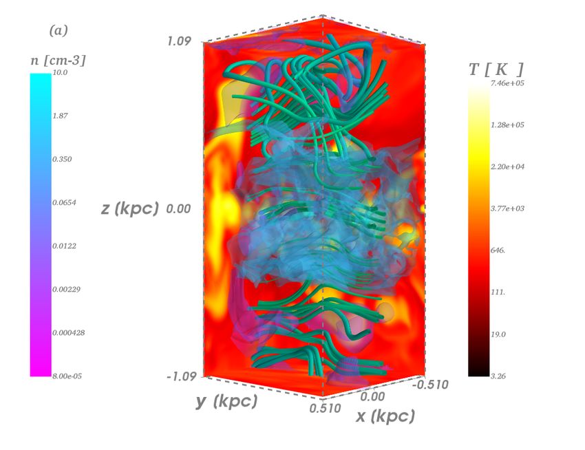
A&A proofs: manuscript no. paper

                         max                       min                  simulated ISM are described in detail in Gent et al. (2013a), and
 n     [cm−3 ]          5 – 8.5           7 · 10−6 – 2.7 · 10−4         a summary is included in Appendix B. The coherence and fluc-
 T       [K]      7 · 107 – 3 · 108            135 – 311                tuations of the magnetic field are important to the polarization
                                                                        measurements, so it is useful to decompose the field into the
 B      [µG]            6      –   10                0                  mean field B̄ and fluctuations b, where
 B̄     [µG]          4.6      –   5.5               0
                                                                        B = B̄ + b.                                                      (1)
 b      [µG]            4      –   7                 0
 u    [km s−1 ]      147       –   549               0                  In this model, the entire field is subject to stirring due to the
                                                                        action of the many SN remnants, so the convention of separa-
Table 1: For the 12 snapshots included in the analysis, at intervals    tion into large-scale and turbulent components needs more care-
of 25 Myr, the ranges of gas number density n, temperature T ,          ful consideration. We separate B by volume averaging with a
total B, mean B̄, fluctuating b magnetic field and speed u.             Gaussian kernel (At l = 50 pc scale, see Gent et al. 2013b). In
                                                                        Fig. 2 (left) B̄ fieldlines and (right) b fieldlines are plotted over
                                                                        density isosurfaces on background slices of temperature. With
not chosen to model the actual turbulent diffusivities, as little       this treatment the ‘mean field’, which is what we shall refer
is known about their dependence on the key physical quantities          to as the large-scale has strength and orientation which varies
in the ISM. The analytical estimates obtained in the first-order        with space and time, but is coherent, i.e. similarly oriented, over
smoothing approximation framework (Steenbeck et al. 1966),              scales above about 100 pc. The small-scale field is derived by
however, imply that the magnitude of turbulent diffusion is or-         subtracting the large-scale field from the total field for any given
ders of magnitude larger than the Spitzer molecular values. The         snapshot. So the large-scale field still exhibits spatial structure,
motivation for the used viscosity scheme is to resolve much finer       which would influence polarization fractions (see Sect. 2.3). The
structures in the cool and warm ISM, than would be possible             random field is clearly incoherent and would contribute to de-
with constant diffusivity.                                              polarization. Some indicative values are listed in Table 1 for the
    Note, that the resolution of 4 pc along each side in these sim-     ranges across the MHD snapshots of gas number density, tem-
ulations without magnetic fields (Gent 2012, Table 5.1) yield a         perature, magnetic field and speed.
maximum gas number density for the ISM of about 100 cm−3                     The gas density ρ from each snapshot is used with the radia-
and the fractional volume of the cold gas is 0.4%. The fractional       tive transfer code SOC, as described in Sect. 2.3, to model the
volume of the warm gas is 60%, with hot gas about 28% near              dust temperature distribution, and the magnetic field B is then
the SN active midplane and increasing to 41.5% elsewhere. With          employed when simulating the dust polarization observations.
the magnetic field included (Evirgen et al. 2018) the model frac-       From the velocity field we can compute directly its divergence,
tional volume of the warm gas increases to about 80%, the hot           ∇ · u, which is also used in the analysis of the polarization to
gas being pushed further into the halo, and the cold gas is con-        determine the influence of the shock structure of the ISM on the
fined to an even smaller fractional volume. A snapshot of the           observations.
thermodynamic profile of the model ISM is displayed in Fig. 1                The simulation used for this analysis applies parameters for
(left), wherefrom the distribution of the different gas phases is       gas density, stellar and dark halo gravitation, galactic rotation,
evident. Observed densities and those arising from the MHD              and SN rates and distribution matching estimates for the Solar
simulations of Hennebelle et al. (2008) extend to much higher           neighbourhood. The magnetic field is amplified for a period ex-
densities and increased fractional volume of cold ISM. The char-        ceeding a Gyr by dynamo action from a seed field of a few nG,
acteristic properties of the MHD simulation data are listed in Ta-      which then saturates with an average field strength of a few µG.
ble 1. Temperatures, velocities and magnetic field strengths are        The strength of the mean field portion is consistent with obser-
better representatives of the observed ISM, but smallest scales of      vational estimates, while the random field strength is 2–5 times
their fluctuations are limited by the grid resolution. The satura-      weaker than estimated. This has some influence on the disper-
tion of the magnetic field has the effect of restricting the flow and   sion of polarization angles in the simulated observations, dis-
increasing the homogeneity of the ISM, so that the maximum              cussed in Sect. 4. We use 12 snapshots from the saturated sta-
density reduces to about 10 cm−3 , which must be taken into ac-         tistical steady stage of the model, each separated by 25 Myr,
count when making comparisons with the Planck observations              commencing at 1.4 Gyr. For simulated maps presented in this
and the earlier MHD molecular cloud model. Mach number in               paper, we use the snapshot at 1.7 Gyr. The system is in a statis-
the simulations reaches as high as 25.                                  tical steady state, so individual snapshot characteristics are rep-
    Both large- and small-scale dynamo instabilities are present        resentative, but strong temporal and spatial differences are also
in the system. A 3D rendition of the magnetic fieldlines embed-         present. For some of the analysis we consider ensemble averages
ded in this atmosphere is illustrated in Fig. 1 (right). As reported    of the snapshots to identify the most persistent structures.
by Evirgen et al. (2017), the strength of the generated mean mag-
netic field at the midplane in the MHD model is in good agree-          2.2. Stellar radiation field
ment with the global observational estimates of 1.6µG by Rand
& Kulkarni (1989), using pulsar RM. The random field in the             Dust in the ISM is illuminated by the stellar radiation field. We
model, however, is much weaker than observed, being only 20–            invert the measurements of the average stellar radiation field in
50% of the 5µG estimate of Rand & Kulkarni (1989) or 5.5µG of           the solar neighbourhood from Mathis et al. (1983) into a dis-
Haverkorn (2015), combining RM with thermal electron density            tribution of radiation sources, to model the stellar radiation for
measures. These estimates are supported by the reviews of galac-        our radiative transfer model. We then model this radiation with
tic magnetic fields (Beck et al. 1996; Beck 2016). Some prelim-         a horizontal density profile (see Gent et al. 2013a, excluding the
inary results applying synthetic RM measurements to the MHD             dark matter component), and emissivity jν reflecting the vertical
model considered here are reported in Hollins et al. (2017), and        distribution of stars as
further such application shall be considered in future work. The                                q
model and the characteristics of the multi-phase structure of the        jν (z) = jν,0 exp a1 za − z2a + z2 .                          (2)

Article number, page 4 of 21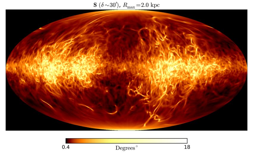
M.S. Väisälä et al.: The SN-regulated ISM. IV. Simulated polarization

Here a1 = 4.4 · 10−14 km s−2 , za = 200.0 pc and jν is the emissiv-      are then finally converted to maps of polarization fraction and
ity over the spectrum of frequencies ν. The normalization coeffi-        polarization angle dispersion. A representative set of synthetic
cients, jν,0 , are determined to return the expected total intensity     Stokes I, Q, and U maps is presented in Appendix A.
Jν from                                                                      To calculate the polarization within a single cell, we ap-
                                                                         ply the following method. We use the Planck/HEALPix conven-
          i=N
        V X jν (zi , jν,0 = 1) −τi                                       tion for the polarization angle ψ (Planck Collaboration Int. XIX
Jν =                          e                                   (3)    2015; Planck Collaboration Int. XXI 2015). Within a cell we
       4πN i        4πd
                                                                         normalize the direction of the magnetic field,
              √
where d = z2 + r2 , V = 2πZ0 R20 and τ is the optical depth                      B
along the line of sight (LOS). The distribution is generated us-         B̂ =                                                                 (4)
                                                                                kBk
ing Monte-Carlo method, and it is scaled to match Jν,Mathis from
Mathis et al. (1983). Using this inversion, we obtain an approx-         and calculate ψ with
imate z-dependent radiation field, which produces reasonable                    π
dust temperatures with our radiative transfer simulations.               ψ=       + arctan(B̂ · φ̂, B̂ · θ̂)                                  (5)
                                                                                2

2.3. Radiative transfer calculations                                     where the φ̂ and θ̂ are the directional vectors of the HEALPix
                                                                         coordinate directions. The angle between the magnetic field and
To calculate the dust emission, we use the program SOC, which            the plane-of-the-sky (POS) is
is a new Monte Carlo code for continuum radiative transfer
against the CRT program (Juvela 2005) and also against several           cos2 γ = 1 − (B̂ · D̂)2 ,                                            (6)
other codes participating in the TRUST1 benchmark project on
3D continuum radiative transfer codes (Gordon et al. 2017). The          where D̂ is the direction of the LOS. Based on the non-polarized
density distribution of the models can be defined with regular           emitted intensity of the cell, Iorig , we get the Stokes components
or modified Cartesian grids or hierarchical octree grids. In this        I, Q and U with
paper, all calculations employ regular Cartesian grids. In addi-                  "
                                                                                                    2
                                                                                                      !#
tion to the density field, the program needs a description of the        I = Iorig 1 − p0 cos γ −
                                                                                              2
                                                                                                                                         (7)
dust grains (i.e. absorption and scattering properties) and of the                                  3
radiation sources. The program employs a fixed frequency grid
to simulate the radiation transport at discrete frequencies, one         Q = Iorig p0 cos(2ψ) cos2 γ                                          (8)
frequency at a time. The information of the absorbed energy is
used to solve the grain temperatures for each cell of the model.
The dust model could also include small stochastically heated
grains. However, to predict dust emission at submillimetre wave-         U = Iorig p0 sin(2ψ) cos2 γ.                                         (9)
lengths, the calculations are here limited to large grains that are
                                                                         To match the polarization degrees observed in the PlanckXIX
assumed to remain at a constant temperature, in an equilibrium
                                                                         and PlanckXX we set p0 = 0.2.
with the local radiation field. Once the dust temperatures have
                                                                             From the integrated Q and U we can calculate the polariza-
been solved, synthetic images of dust emission can be calculated
                                                                         tion fractions p and the polarization angle dispersion functions
towards selected directions or, as in the case of the present study,
                                                                         S over the whole sky. Simulated p and S yield familiar measures
over the whole sky as seen by an observer located inside the
                                                                         of system properties and allow comparison to previous studies.
model volume.
                                                                         The polarization fraction is defined as
     We assume a constant gas-to-dust ratio, where we follow the
dust model BARE-GR-S of Zubko et al. (2004), which has been                    p
                                                                                 Q2 + U 2
created to match the observations of typical Milky Way dust with         p=                                                          (10)
the extinction factor Rv = 3.1. For simplicity, we keep the prop-                   I
erties of the dust similar throughout the whole computational do-        and the polarization angle dispersion function (Falceta-
main. Dust properties may vary between different ISM phases,             Gonçalves et al. 2008; Hildebrand et al. 2009; Planck Collab-
but the investigation of these effects is beyond the scope of this       oration Int. XIX 2015) as
initial study.                                                                     v
                                                                                   u
     During the simulation of the internal radiation field, the ra-                       N
                                                                                   t
                                                                                       1 X
                                                                         S(r, δ) =           ψ(r) − ψ(r + δi ) 2 ,

diation transport is calculated without taking the polarization                                                                   (11)
into account. However, SOC includes tools to produce synthetic                         N i=1
polarization maps. The local grain alignment efficiency could
be calculated following the predictions of the radiative torques         where ψ(r) is the polarization angle in the given position in the
theory (Draine & Weingartner (1996); Pelkonen et al. (2009);             sky r and ψ(r + δi ) the polarization angle at a position displaced
PlanckXX). Because our study concentrates on emission from               from the centre by the vector δi . The sum extends over pixels
low-density medium, this step is omitted and we essentially as-          whose distances from the central pixel in the location r are be-
sume a constant dust grain alignment efficiency. The polarization        tween δ/2 and 3δ/2. As in PlanckXIX, we calculate the disper-
reduction factor p0 is simply set to a constant value that results       sion function with:
in a maximum polarization fraction that is consistent with obser-                                1
vations. Maps are calculated separately for the Stokes I, Q, and         ψ(r) − ψ(r + δi ) =       arctan(Qi Ur − Qr Ui , Qi Qr + Ui Ur ).   (12)
                                                                                                 2
U components, taking into account the local total emission, the
local magnetic field direction, and the value of p0 . These data         In addition, to be comparable with the analysis presented in
                                                                         PlanckXIX we apply 1◦ Gaussian smoothing to our simulated
1
    http://ipag.osug.fr/RT13/RTTRUST/                                    observations, and set δ = 300 for all calculations of S. This sets
                                                                                                                     Article number, page 5 of 21
A&A proofs: manuscript no. paper

the widest distance between points in the annulus to be 1.5 times             yielding the composite 2D-histograms, as presented in Fig. 3 and
the size of the FWHM of the Gaussian filter. The size of the an-              subsequent 2D-histogram figures. Combined 2D-histograms,
nulus is small because, according to PlanckXIX the angle dis-                 summing counts over many snapshots and POV, contain the pat-
persion function S gradually loses its coherence with increasing              terns most consistent across the individual 2D-histograms. De-
δ. PlanckXIX also note that their measurements of S are not an                spite masking low count noise, many low-frequency outliers per-
artefact of either the choice of δ itself or instrumental bias. How-          sist.
ever, the small annulus will include some influence due to spatial                 The various simulated observations may each exhibit distinct
correlations induced by the 1◦ beam. The choice of δ is indepen-              features worthy of further analysis in the future. However, in this
dent of our radiative transfer model, and its primary justification           study we focus on the general behaviour of the system. For ex-
is to compare our results with PlanckXIX.                                     ample, the 2D-histograms only include pixel-by-pixel numerical
     We have calculated our results with several integration dis-             values. Therefore, such analysis cannot regard the filament-like
tances Rmax , namely Rmax = 0.25, 0.5, 1, 2, 4 kpc, to explore the            shapes visible in S-maps (See Figs. 9, 5 and 14).
effect of depth. A part of the emission observed in Planck XIX
is received from distances larger than what our model is capa-                3. Properties of synthetic polarization observations
ble of exploring However, with this in mind, our motivation is
to inform, with an independently and physically generated ISM                 Here we present our results and analysis based on the synthetic
and magnetic field, how the impact of near and distant features               observations obtained using SOC with polarization tools on top
might contribute to the observed images. We assume periodic                   of our MHD simulations. For our analysis, we use the maps of
boundary conditions in the horizontal direction of the computa-               column densities NH , polarization fractions p and polarization
tional domain. However, if the boundary is crossed in the ver-                angle dispersions S. As discussed in Sect. 2.1, we take (in the
tical direction, the integration stops at that point, as happens in           figures) as the reference case the 1.7 Gyr snapshot, where the ob-
the cases Rmax = 2 and 4 kpc. Note, for our analysis, we mask                 server is situated in the centre of the computational domain. We
latitudes |b| > 45◦ from our maps. This more closely reflects the             opt for projection onto a sphere as the most appropriate observa-
region of the sky where the Planck observations are included in               tional reference frame. With the domain spanning over 1 kpc in
the analysis of PlanckXIX. This is an arbitrary choice, as we are             each direction, it is too large to be treated as a single observation
not limited by the signal-to-noise issues of PlanckXIX. However,              along a Cartesian coordinate. Thus, projection onto a sphere is
this has also other benefits. It avoids the problem of calculating            the most realistic observational frame, and especially so when
S near the poles and some of the issues of asymmetry, caused by               nearby regions are concerned. The all-sky point of view affords
the limited vertical extent of the domain, that would affect the              the best comparison with Planck on the scales relevant to the
comparison of Rmax ≤ 1 kpc and Rmax ≥ 2 kpc. To save space,                   MHD model. All of the maps of synthetic observations over the
we omit from the figures related to the case with Rmax = 0.5 kpc,             whole sky are presented using Mollweide projection.
but the results are similar to Rmax = 1 kpc.

2.4. Combining data into 2D-histograms                                        3.1. Simulated column density
Many of the results in this paper are represented using joint 2D-                 The maps of column density resulting from integrating over
histograms. This allows us both to compare our results directly               each distance, up to Rmax = 0.25, 2 and 4 kpc from the observer,
to the analysis in PlanckXIX and PlanckXX, and separate the                   are shown in Fig. 3, right panels. The dependence of NH on Rmax
snapshot and point-of-view (POV) specific details from the gen-               is immediately apparent. The densest regions are situated near
eral large-scale behaviour.                                                   the midplane, as would be expected from horizontal averaging of
     For 2D-histograms, we combine radiative transfer simu-                   the gas density in the MHD model represented in Fig. 1. How-
lations from all 12 snapshots and for 5 different POV po-                     ever, this is not visible on the map from Rmax = 0.25 kpc, but
sitions in the approximate midplane, specifically from the                    clear for the higher Rmax . The vertical anisotropy in the latter re-
points (0.5, 0.5, 1.0) kpc, (0.25, 0.5, 1.0) kpc, (0.5, 0.25, 1.0) kpc,       flects the temporal upward shift of the disk centre of mass, evi-
(0.75, 0.5, 1.0) kpc and (0.5, 0.75, 1.0) kpc, under the assump-              dent from Fig. 1. Also, density should be near isotropic in the lat-
tion that the use of periodic boundary conditions in x- and y-                itudinal direction, because we do not model the galaxy’s central
directions should give a reasonable representation of the ISM in              bulge nor spiral arms. In a single snapshot, however, local SN
the neighbourhood of the Solar System.                                        bubbles or superbubbles (merging multiple SN remnants) may
     The data is combined as follows. From each SOC-generated                 inject significant anisotropy into the overall density profile. This
map, i=1-60, separate 2D-histograms are constructed over a                    is clearly seen only for the Rmax < 1 kpc, with bubbles apparent
common set of 512 × 512 bins for each comparison, specifically                on several locations. For the higher lengths of integration the in-
Cbin,i (NH , p), Cbin,i (NH , S), Cbin,i (p, S). Here Cbin,i represents the   fluence of features near to the observer is almost negligible. As
number of counts in a single bin calculated from a single syn-                the combination of nearby and far-away emission will be present
thetic observation. Then, assuming Cbin,i to be lognormally dis-              in both real and synthetic observations, exploring the effect of
tributed between separate 2D-histograms, we calculate the mean                distance to the observations is called for.
and standard deviation over i,                                                    Fig. 3, left panels, show joint 2D-histograms of polariza-
                                                                              tion angle dispersion S and column density NH for Rmax =
log Cbin = hlog Cbin,i i,   σlog Cbin = σ(log Cbin,i ).               (13)    0.25, 2 and 4 kpc. At 0.25 kpc, NH is clustered around only
                                                                              1.5 · 1020 cm−2 and S < 1◦ , while its corresponding NH map,
   We include only the bins Cbin for which Cbin,i > 0 for all i.              dominated by local gas structure, is without dense clouds. This
Second, to reduce additional noise, we mask out the elements                  is inconsistent with PlanckXIX and indicates that the integra-
where                                                                         tion length is too short. For higher Rmax , NH is typically above
                                                                              1021 cm−2 and consistent with the observed column density fea-
exp(log Cbin − σlog Cbin ) < 5,                                       (14)    tured in PlanckXIX, Fig. 24 upper panel. S also increases above
Article number, page 6 of 21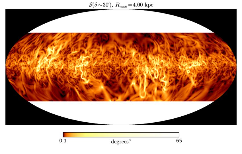
M.S. Väisälä et al.: The SN-regulated ISM. IV. Simulated polarization

Fig. 3: Left: Joint 2D-histograms of polarization angle dispersion S and column density NH . The green lines follow the maximum
Cbin as a function of NH , and the blue lines present the weighted mean of S. Right: Sample maps of column density. For the case
Rmax = 1 kpc, see Fig. 13.

1, but not to the level obtained by PlanckXIX. The high Rmax          smooth out structures, also those seen in S, more efficiently, that
maps of NH also capture the presence of these clouds, particu-        is a relation S ∝ νt−1 would be expected, where νt is a turbulent
larly evident near the midplane.                                      diffusion coefficient related to turbulent mixing, not necessar-
    On these joint 2D-histograms are also plotted lines of maxi-      ily to any dependence assumed in viscosity scheme used in the
mum Cbin (green) and weighted mean (blue) polarization frac-          model. As explained in Sect. 2.1, gas viscosity is set as ν ∝ T 0.5
tions as functions of NH . For Rmax & 1 kpc the trend has a           so as to resolve flows in the hot gas of the MHD model. The
positive correlation with NH , in disagreement with PlanckXIX         ISM is modelled as an ideal gas, with all phases in approximate
Fig. 24. There is no record in PlanckXX on how this relationship      statistical pressure balance, so this is statistically equivalent to
applies to their MHD model. Comparing our synthetic observa-          ν ∝ ρ−0.5 . For the radiative transfer calculations, the dust den-
tions with PlanckXIX Fig. 24, there is a peak in the weighted         sity is assumed proportional to the ISM gas density. If higher
mean profile for high column density dust. This corresponds to        viscosity in the hot gas tends more proportionally to smooth
the molecular clouds, which are not resolved in the MHD model.        small-scale structures in the flow, we might expect the disper-
In Fig. 3 (Rmax > 1 kpc) the high column density range, repre-        sion S ∝ NH0.5 , which we indeed see for the low-density hot gas.
senting the warm and cold ISM, is a good match for the Planck-        This implies that the diffusion in the hot gas reflects the depen-
XIX data. In the PlanckXIX data, however, the weighted mean           dence input through the viscosity scheme, while the one for the
remains as high or even increases at lower densities, while our       cold and warm gas does not do so, but is somewhat steeper than
simulations show a correlation S ∝ NH0.5 in this range of column      expected from this simple argumentation.
densities, being in obvious disagreement.                                  We have no reliable method to determine observationally
    Let us try to understand this discrepancy by assuming that the    what is the true turbulent viscosity in the ISM. Some elabo-
small-scale scatter seen through S is a result of the underlying      rate and approximate methods make this possible within nu-
turbulent diffusion, taking the action of smoothing the flow. If      merical experiments (see, e.g., Käpylä et al. 2018). Our sim-
this was the case, one would expect the higher viscosity regions      ple hypothesis presented above could be tested by applying the
                                                                                                              Article number, page 7 of 21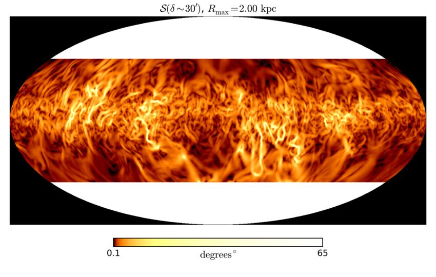
A&A proofs: manuscript no. paper

same analysis in this paper to MHD simulations with alterna-               Regardless of these current limitations, it is interesting to
tive prescriptions for viscosity, to exclude a relationship between   consider how the distances influence polarization and depolar-
the weighted mean profile and the viscosity, as appears to exist      ization. In the framework of the radiative transfer calculations,
here. However, if MHD models consistently display such a de-          the mechanism is easy to understand. Along the LOS, individual
pendence on viscosity S ∝ ν−1 for the weighted mean S, then           cells in the grid produce positive and negative contributions in Q
we might be able to infer something about the actual turbulent        and U, depending on the local magnetic field direction. For an in-
viscosity in the ISM from the PlanckXIX profiles. Using Planck-       coherent magnetic field, the sign of Q and U fluctuates, with sim-
XIX with the weak negative correlation in between the weighted        ilar magnitude, such that over very long distances in an optically
mean values of S and NH would imply ν ∝ T −λ for the ionized          thin medium their averages approach zero. This is comparable to
ISM, with 0 < λ  1. This is quite unlike, e.g., Spitzer molec-       the analysis of Houde et al. (2009), where they note that multiple
ular viscosity ν ∝ ρ−1 T 2.5 . The scale of such simulations place    independent turbulent cells along the line of sight will make the
that investigation beyond the scope of the present study, and of      apparent fluctuation to approach zero. However, the mean field
course there are many complicating factors which would permit         also varies in direction when exploring kiloparsec scales which
alternative explanations of this trend.                               will also contribute to the perceived effect. In the presence of a
    At the lowest Rmax the visible cloud structure in the NH map      directionally coherent magnetic field, its direction will dominate
is directly tracing our MHD model. With increasing Rmax smaller       the Q and U over long distances. However, the magnetic fields
details appear in the maps, which are the effects of projection       are highly turbulent throughout the MHD domain, so we expect
from more remote sources. Hence, the observed results are in-         depolarization to increase with Rmax .
evitably a combination of both the MHD model volume and                    Near the midplane the depolarization effect is strongly pro-
its projection through a mixture of features along the LOS. By        portional to integration length with Rmax ≥ 2 kpc (Fig. 4, lower
assuming periodicity in the horizontal direction, we can reach        right panels), corresponding high NH . This is also consistent with
higher Rmax than the physical scale of our MHD model. How-            the above explanation. Near the midplane with large Rmax it is
ever, with too high Rmax the periodicity creates a mirror gallery     possible to integrate polarization over a longer distance, unlim-
effect of repeating patterns near the x- and y-axes of the MHD        ited by the upper or lower boundaries of the computational do-
model. To avoid this, it is reasonable to restrict the highest in-    main. Therefore, there is more influence on p from the depolar-
tegration distance to Rmax = 2 kpc, or for the general case,          izing effect of the fluctuations, most evident near the midplane.
Rmax . 2L x , where L x is the horizontal extent of the MHD           The role of magnetic field fluctuations inducing a broad spread
model.                                                                of p has also been suggested by PlanckXIX and PlanckXX and
3.2. Polarization fraction across the galactic plane                  our results support this idea.
                                                                           Due to the averaging and masking method presented in
For each Rmax we construct joint 2D-histograms of polarization        Sect. 2.4 some of the outlying values persist as halos in the 2D-
fraction p and NH , presented in Fig. 4, left panels, and the maps    histograms of Fig. 4 (also Fig. 13), but with higher sampling
of p, right panels. With Rmax = 0.25 kpc there is a broad range for   rates, the masked points between the bulk data and halo could be
p values. The distribution is independent of the NH values, which     restored. Also, the gradual loss of alignment of the dust grains
in this case are much lower than in the PlanckXIX observations.       within radiation shielded dense clouds can decrease polarization,
The mapping of p can be seen to correlate over large smooth           which is also considered by PlanckXIX to be an effect influenc-
regions. There is negligible depolarization, with the highest Cbin    ing their observed depolarization with NH ≥ 1022 cm−2 . We set
appearing on the scale of p0 = 20%.                                   the strength of alignment proportional to p0 in Eqs. 7-9, neglect-
    With Rmax = 2 kpc depolarization is stronger, particularly        ing any effects of such shielding.
near the midplane, the map of p being an excellent analogue                As our methods resemble those of PlanckXX, some dicus-
for PlanckXIX, Fig. 6. Its 2D-histogram is also a better match        sion is called for, although we cannot make a direct comparison
with PlanckXIX, Fig. 19, although NH > 1022 cm−2 are absent           of their MHD model with our results. They consider scales well
and there are few values with p > 15%. The high column den-           below our 4 pc grid resolution. What is relevant, is that the struc-
sity may relate to features not modelled with the MHD, such as        ture of the flow and the magnetic field in our MHD model is
the central bulge, spiral arms, and molecular cloud properties re-    naturally driven by the forces on the scales of SN remnants cas-
quiring higher resolution to be resolved. Some of the absence of      cading to the lowest turbulent eddies we can resolve. It is reason-
higher p is due to the masking of bins which lack signal across all   able to expect that the turbulent structure would extend to lower
synthetic maps cobined to the 2D-histogram in question. In ad-        scales, until new physical processes become active.
dition, the fraction of the PlanckXIX data, which has p > 15%,             PlanckXX compare their MHD results with observations of
is concentrated into the molecular cloud complexes, where high        the Chamaeleon-Musca and Ophiuchus fields. For their MHD
polarization fractions can be found, which are among the fea-         simulation, they view the domain with respect to the mean field
tures not resolved in our MHD models.                                 as POS, LOS and 50/50, confirming that a high polarization
    The increased frequency of p > 5% with Rmax = 4 kpc is            fraction is indicative of a strong POS component to the field.
more like the PlanckXIX results, but the high number of points        This is evidence that the magnetic field has a strong POS com-
where p < 5% and NH ' 5 · 1021 cm−2 is not consistent with            ponent in Chamaeleon-Musca, while in Ophiuchus the field is
PlanckXIX, and an indication that oversampling the same peri-         more aligned along the LOS, an interpretation consistent with
odic domain near the midplane is distorting the distribution. To      Planck Collaboration Int. XXXV (2016), their Fig. 3, which
improve the range of column densities in a physically consistent      shows a more consistently ordered POS field for Chamaeleon-
manner, one should increase the horizontal extent of the MHD          Musca compared to that of Ophiuchus.
models. Also, increasing the MHD model resolution would im-                For all three cases examined in PlanckXX, the values in
prove both the proportion of high column densities and high po-       the polarisation fraction distribution are low compared to either
larization fractions, but this would be computationally demand-       Chamaeleon-Musca or Ophiuchus. It may be that the random
ing in the context of SN-driven MHD turbulence that is capable        component, and hence depolarization, in the MHD models was
of producing self-consistent small- and large-scale dynamos.          too strong. Alternatively, the forcing mechanism they use in-
Article number, page 8 of 21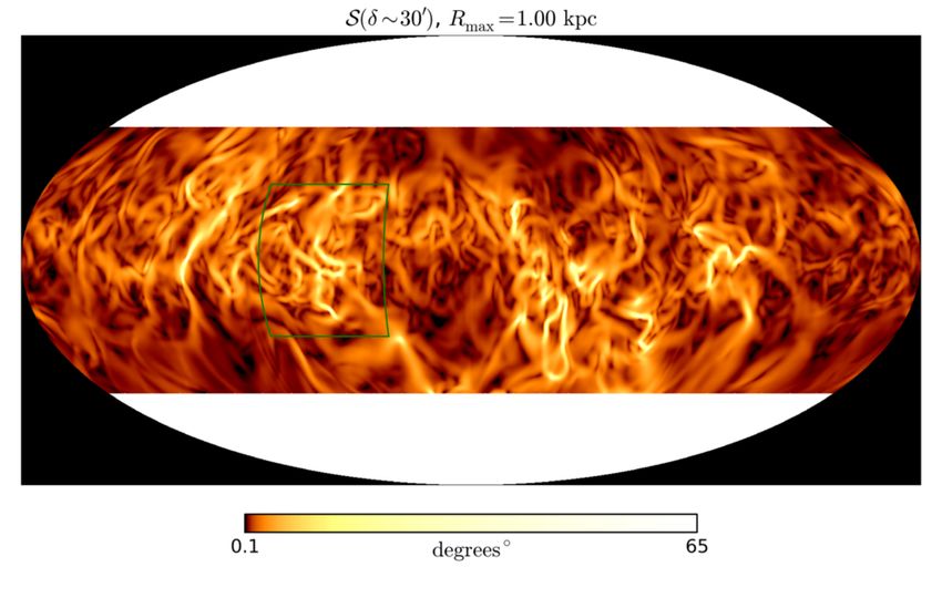
M.S. Väisälä et al.: The SN-regulated ISM. IV. Simulated polarization

Fig. 4: Left: Joint 2D-histograms of polarization fraction p and column density NH . Red dashed lines show the location of pmax =
19.8% from PlanckXIX. The green lines follow the maximum Cbin as a function of NH , and the blue lines present the weighted mean
of p. Right: Sample maps of p. The polarization fractions are weakened in the galactic midplane, which is seen in the 2D-histograms
as a growing distribution of low p at high NH . For Rmax = 1 kpc, see Figs. 14 and 13.

duced a Gaussian distribution to the magnetic field, while our        3.3. Polarization angle dispersion
analysis, with SN-driven turbulence, indicates it to have more
exponential distribution, which could influence the efficiency of     Looking at the maps of polarization angle dispersion S presented
the depolarization (see Sect. 3.3). With respect to the mean field    in Fig. 5 (right panels), we observe filamentary structures (S-
component Gent (2012, Ch. 9 Fig. 9.12), find that the magnetic        filaments) similar in appearance to PlanckXIX Fig. 12. However,
fields in the cold filamentary regions formed by SN driven turbu-     for Rmax = 0.25 kpc these are very large scale structures, which
lence are more regular than the ISM as a whole and that they are      span the full range of examined galactic latitudes in some lo-
strongly aligned with the ambient warm ISM, in which they are         cations and are much thicker than the PlanckXIX observations.
embedded. This is in contrast to the observations of Planck Col-      With increasing Rmax the S-filament structure resembles quite
laboration Int. XXXII (2016); Planck Collaboration Int. XXXIII        well PlanckXIX Fig. 12, becoming tangled and fragmented, in-
(2016), who found the orientation of the filamentary structure of     creasing in number and having more wiggles. PlanckXX report
the most dense molecular clouds to be perpendicular to the mean       filament-like maps of S from their synthetic observations. How-
magnetic field. Here, gravitational collapse and runaway thermal      ever, due to the differences in scale, resolution and forcing mech-
instabilities leading to the formation of such high density struc-    anism behind the MHD model used in PlanckXX and this study,
tures may be critical, which are absent on the scales considered      an effective qualitative comparison is not reasonable.
in our MHD model.                                                         In Fig. 5 (left panels) the joint 2D-histograms of S and p
                                                                      show some agreement with Fig. 23 of PlanckXIX. Angular dis-
                                                                      persion is inversely proportional to polarization fraction, and
                                                                      may be approximated by
                                                                      log10 S = α log10 p + β.                                      (15)
                                                                                                             Article number, page 9 of 21
A&A proofs: manuscript no. paper

Fig. 5: Left: Joint 2D-histograms of angle dispersion and polarization fraction, with the effect of increasing Rmax . The red line depicts
the fit to the observations as presented in PlanckXIX, log10 S = α log10 p + β. The black lines are the best fits to our simulated data,
to which α and β are given in the Table 2. Right: Sample maps of polarization angle dispersion S with corresponding Rmax .

    Rmax (kpc)          α            β   hS/SPlanck i      Notes         zontal extent and/or increased resolution might indicate whether
             –     −0.834       −0.504       100%          Planck        this is a robust physical relationship between the simulated and
          0.25     −0.673       −0.961         24%                       observed measurements. The ratio S/SPlanck = pα−αPlanck 10β−βPlanck
           0.5     −0.742       −0.898         32%                       is averaged and listed in Table 2 for each Rmax .
           1.0     −0.789       −0.920         34%                            The dispersion values in our simulations increase towards
           1.0     −0.934       −1.020         39%         2·b           PlanckXIX as Rmax increases, but plateau at a ratio of 35% for
           2.0     −0.876       −0.999         35%                       Rmax & 1 kpc. The increase to 39%, when artificially strengthen-
           4.0     −0.892       −1.021         35%                       ing the amplitudes of the small-scale fluctuations of the magnetic
                                                                         field, supports the view that the low simulated value for β is in
Table 2: Fits to log10 S = α log10 p + β for each joint 2D-              part due to insufficient small-scale field. The low values of S in
histogram of S and p. The observed values are from the best              our MHD model may be attributed to truncated resolution at the
fit of PlanckXIX.                                                        grid scale of 4 pc.
                                                                              To understand the distribution of velocity and magnetic fields
                                                                         in our MHD model data, we present probability density distri-
The 2D-histograms show our best fits (black lines) for Eq. (15)          bution functions (PDFs) of the both variables in Figs. 6 and 7.
and the fit from PlanckXIX (red lines). The parameters are sum-          The PDFs are calculated over all MHD model cells from all
marised in Table 2. For Rmax at 1 kpc and above, the slope α             snapshots where each cell, being of same volume, has an equal
is near to the PlanckXIX fit, but by having smaller intercept β          weight. In Fig. 6, upper panel the PDF is exponential for Bx
our 2D-histograms are shifted to lower S. There may be a case            (By ) and Bz , while By (Bx ) is skewed by the global shear. Fig. 6,
for inferring that the optimal integration length is about Rmax =        lower panel, shows the PDFs for the velocity components, where
1.5 kpc, if we are looking to match α for the PlanckXIX data.            within the velocity range ±400 km s−1 , the PDFs reflect ISM
Repeating the analysis for an MHD domain with increased hori-            physics as resolved by the model. We evolve SN remnants only
Article number, page 10 of 21
M.S. Väisälä et al.: The SN-regulated ISM. IV. Simulated polarization
from the latter stages of the Sedov-Taylor phase, however, so this 10-1
is exhibited in the truncated PDF for |u| & 400 km s−1 . Bx
The spiked PDF displayed in Fig. 6 for the magnetic and 10-2 By
velocity field components arise from the physics of repetitive
shock-driven turbulence, independent of the model and resolu- 10-3 Bz
tion. Few authors have discussed this property, but a similar dis-
tribution for the velocity profile is illustrated in Gressel (2010, 10-4
P(Bi )
Fig. 3.13). In their Fig. 9 Mac Low et al. (2005), using approx-
imately 1.5 pc resolution, show similar PDF profiles for the di- 10-5
vergence of the velocity field, also supporting this physical in-
terpretation of the turbulent structure of the ISM. 10-6
The multiphase medium plays a role in this distribution. In
Fig. 7 we divide PDFs into three components, corresponding 10-7
with cold, warm and hot medium (T < 100 K, 100 ≤ T < 105 K
and T > 105 K respectively). The Fig. 6 velocity profile mainly 10-8 10 5 0 5 10
exhibits the warm phase PDF depicted in Fig. 7, apart from at B (µG)
high velocities where the hot phase is more visible. The PDF is
approximately Gaussian for the cold phase. Based on this com- 10-1
ponent separation, the sharp PDF profile of magnetic field in the ux
hot phase, and less so for the warm, is likely connected with the 10-2 uy
large-scale compressive forcing in the warm and hot phases, and uz
subsequent turbulent cascade. The cold phase contains a mag- 10-3
netic field with a distribution that is between an exponential and
a Gaussian, resembling that of PlanckXX, Fig. 11, apart from 10-4
P(ui )
having a weaker magnetic field strength. It is possible that the
higher densities in the cold phase may act as a sponge for these 10-5
compressions and rarefactions, but we cannot assume that the
effects of the turbulent cascade driven by SN are absent even at 10-6
the scale of molecular clouds.
10-7
Therefore, some caution should be attached to the velocity
PDF for the cold phase for at least two reasons. In their Fig. 15 10-8 600 400 200 0 200 400 600
(c) Gent et al. (2013a) show that the hot phase flows are mainly
subsonic, the warm transonic and the cold supersonic. However, u (km/s)
the cold clusters are typically entrained within the bulk flows
of their ambient warm gas. If the bulk velocity of the ambient Fig. 6: Probability density function combined from all 11 snap-
warm gas were subtracted, then the Mach number of the cold shots for the components of B and u.
phase would likely reduce, and the residual flow might retain
more of the PDF structure of the hot and warm phases. Also,
in this model the scale of the cold structures tend to be only a 4.1. S-filaments compared with shocks
few grid spaces across, i.e., they are near the limit of the model
resolution, so much of the substructure of the magnetic and ve- Changes in the direction of polarization angle ψ and therefore S
locity fields in this phase are truncated. So although the MHD are related to changes in the magnetic field, and these are driven
model here is truncated at 4 pc, it is our contention that the and generated by SN-driven turbulence. Generally, S follows a
physics that drive the structure of the magnetic field in the hot lognormal distribution (see PlanckXIX Fig. 14). The lognormal
and warm phases are still relevant to the flow driving the dy- nature of the S distribution in the observed and simulated ISM
namics at smaller scales. This would require comparison with appears consistent with the effect shocked turbulence has on the
higher resolution multi-phase turbulence simulations. Only from statistics of the gas density (as noted in Vazquez-Semadeni 1994;
new physical processes, such as self-gravity, would we expect to Elmegreen & Scalo 2004; Gent et al. 2013a), which encourages
introduce changes to the structure of the turbulence. us to look into the connection between S distribution and shocks
present in our simulation data.
To investigate the effect that the shocks have, we first com-
pute a proxy of their magnitude, Cshock,local = |[∇ · u]− |, where
4. Shock and magnetic structure interpretation only the negative divergence contributes. This corresponds to re-
gions where the flow is convergent, where therefore the shocks
We now consider how S-filament structures seen in the polariza- created by SNe are compressing the surrounding ISM. The val-
tion angle dispersion measurements are related to physical prop- ues of Cshock,local are calculated within the numerical grid of the
erties of the ISM. These are difficult to measure directly through MHD model. All Cshock maps show Cshock,local averaged over the
observations, but can be measured easily in the MHD models. LOS up to the defined Rmax , or
In the analysis that follows, we mostly refer to integration along
the LOS with Rmax = 1 kpc. This range, within the properties and Rmax
horizontal extent of the MHD model, is sufficient to adequately Cshock = hCshock,local iLOS . (16)
0
capture the key features present in the PlanckXIX observations.
For more demanding analysis it would be recommended to inte- In Fig. 8, maps are displayed for average Cshock , S, and the POS
grate Rmax ' 2L x . magnetic field, |BPOS |, averaged over the LOS up to Rmax =
Article number, page 11 of 21A&A proofs: manuscript no. paper
10-1 10-1 10-1
Bx Bx Bx
10-2 By 10-2 By 10-2 By
10-3 Bz 10-3 Bz 10-3 Bz
10-4 10-4 10-4
P(Bi )
P(Bi )
P(Bi )
10-5 10-5 10-5
10-6 10-6 10-6
10-7 10-7 10-7
10-8 10 5 0 5 10 10-8 10 5 0 5 10 10-8 10 5 0 5 10
B (µG) (TM.S. Väisälä et al.: The SN-regulated ISM. IV. Simulated polarization
set of galactic magnetic field models without dynamo nor SN-
driven turbulence to generate a realistic field, but including the
galactic centre and spiral arms, which they fit to observational
data. Their synthetic maps do not have the small-scale features
associated with the turbulence, but on larger scales our maps
have very similar structure, the only characteristic difference be-
ing longitudinal variation caused by the included spiral arms. So,
apparently, local structures in the ISM may be predominant in
the observed data, although further investigation along the lines
of Planck Collaboration Int. XLII (2016) and inclusion of spiral
arms in a model of MHD turbulence would need to be pursued.
The large-scale variation follows from the presence of the
mean field in our MHD model. We can illustrate it with a sim-
ple analytical example starting from the first principles. Let us
assume a simple uniform y-directional mean field with random
fluctuations at the smallest scales of the grid
B = B0 ŷ + ∆b (17)
where |B0 ŷ|
|∆b|. This configuration generates a large-scale
structure of the polarization (see Fig. 12, and also Planck Col-
laboration Int. XLIV 2016, their Fig. 4, top panels). In addition
to this, the direction of the magnetic field affects the sensitiv-
ity of the observed polarization to the small magnetic fluctua-
tions. If we apply Eq. 17 to Eqs. 4, 5 and 6 we notice that near
the HEALPix coordinates φ ≈ ±π/2 and θ ≈ π/2 the influence
of the magnetic field approaches the values ψ ≈ π/2 + ∆ψ and
γ ≈ π/2 + ∆γ, where we have divided the contribution from the
mean and the fluctuating field. Therefore, when calculating the
polarization components, with Eqs. 8 and 9, we get,
Q ≈ −I p0 cos ∆ψ sin2 ∆γ (18)
U ≈ −I p0 sin ∆ψ sin2 ∆γ. (19)
This signifies that, when the LOS approaches the direction of the
consistent mean magnetic field, the POS field is highly sensitive
Fig. 8: Top: The distribution of the average values of Cshock in the to small, local fluctuations caused by turbulence. This, in turn,
LOS. Middle: Map of polarization angle dispersion S. Bottom: will show up as variations in polarization angle and therefore rel-
Projected average magnetic field strength in POS. The green atively high S. To summarize, when the strong mean field is per-
rectangles refer to the area featured in Fig. 9. Rmax = 1 kpc. pendicular to the LOS, its direction dominates the polarization
angles, but when the field is parallel to the LOS, the observed
polarization angles are more sensitive to the small fluctuations
across the galactic plane and also exhibits the same latitudinal in the field. However, the polarization fraction p is weak in the
sign reversals as Q (upper right panel). The polarization frac- mean field aligned with the LOS, as the small fluctuations them-
tions are minimised where the brightest filamentary structures selves produce less strong Q and U. Thus, we have a similar
are most pronounced. The general nature of this pattern may be interpretation to PlanckXX. In their study, S is strongest when
expected. As outlined in Sect. 2.1, the magnetic mean field is the POV faces towards the mean field direction, along with a
strongly aligned in the direction of the differential rotation of the weaker polarization fraction. In contrast, they observe a higher
model. polarization fraction and a coherent polarization angle when the
The dependence of polarization properties on the orienta- direction of the mean field follows the POS.
tion of the mean magnetic field is a known relation. Already, in Note, that B0 ŷ here is distinct from B̄ as defined in Eq. (1).
the context of turbulent molecular clouds, Ostriker et al. (2001), B̄ is defined by local averaging and includes varying x and y
Soler et al. (2013) and PlanckXX have shown that distribution components, although it is most strongly aligned along y. In the
of fluctuations in polarization is connected with the direction MHD model, the fluctuations b have the same order of magni-
of the magnetic mean fields of molecular clouds. Such analysis tude as B̄, which complicates visualising the large-scale mean
has also been utilized with Planck observation in relation to the field even with the simulated observations. For observations, the
molecular clouds (Planck Collaboration Int. XXXII 2016; Soler structure of the mean field is even more opaque, as the mean
et al. 2016). This urges us to look into this phenomenon with our field direction is subject to large-scale diversions when interact-
modelling results. However, as we look into large-scale patterns, ing with spiral arms and the central bulge of the galaxy. There-
Planck Collaboration Int. XLII (2016); Planck Collaboration Int. fore, using this interpretation to understand the observed S by
XLIV (2016) provide the most fruitful points of comparison. PlanckXIX is not trivial. In the case of our MHD simulation, the
The upper panels of Fig. 11 are remarkably consistent with mean field is clearly stronger than the fluctuating field. In the
Planck Collaboration Int. XLII (2016, Fig. 13), who examine a case of our Galaxy, the general structure of the large-scale field
Article number, page 13 of 21You can also read