First Solar Orbiter observation of the Alfvénic slow wind and identification of its solar source
←
→
Page content transcription
If your browser does not render page correctly, please read the page content below
Astronomy & Astrophysics manuscript no. output                                                                                          ©ESO 2021
June 9, 2021

      First Solar Orbiter observation of the Alfvénic slow wind and
                     identification of its solar source
R. D’Amicis1 , R. Bruno1 , O. Panasenco2 , D. Telloni3 , D. Perrone4 , M. F. Marcucci1 , L. Woodham5 , M. Velli6 , R. De
Marco1 , V. Jagarlamudi1 , I. Coco7 , C. Owen8 , P. Louarn9 , S. Livi10 , T. Horbury5 , N. André9 , V. Angelini5 , V. Evans5 ,
A. Fedorov9 , V. Genot9 , B. Lavraud11, 9 , L. Matteini5 , D. Müller12 , H. O’Brien5 , O. Pezzi13, 14, 15 , A. P. Rouillard9 , L.
                     Sorriso-Valvo15, 16 , A. Tenerani17 , D. Verscharen8, 18 , and I. Zouganelis19

      1
          National Institute for Astrophysics (INAF) - Institute for Space Astrophysics and Planetology (IAPS), Via Fosso del Cavaliere,
          100, 00133 Rome, Italy
          e-mail: raffaella.damicis@inaf.it
      2
          Advanced Heliophysics, Pasadena, CA, USA
      3
          National Institute for Astrophysics (INAF) - National Observatory of Turin (OATo), Via Osservatorio, Pino Torinese, Turin, Italy
      4
          Italian Space Agency (ASI), via del Politecnico snc, 00133 Rome, Italy
      5
          Department of Physics, Imperial College London, London SW7 2AZ, UK
      6
          UCLA Earth Planetary and Space Sciences Department, Los Angeles, CA, USA
      7
          Istituto Nazionale di Geofisica e Vulcanologia (INGV), Via di Vigna Murata 605, 00143 Rome, Italy
      8
          Mullard Space Science Laboratory, Holmbury St Mary RH5 6NT, UK
      9
          Institut de Recherche en Astrophysique et Planétologie, Université Toulouse III—Paul Sabatier, CNRS, CNES, Toulouse, France
     10
          Southwest Research Institute, San Antonio, TX
     11
          Laboratoire d’Astrophysique de Bordeaux, Univ. Bordeaux, CNRS, Pessac, France
     12
          European Space Agency, ESTEC (SCI-S), PO Box 299, Noordwijk 2200 AG, The Netherlands
     13
          Gran Sasso Science Institute (GSSI), Viale F. Crispi 7, 67100 L’Aquila, Italy
     14
          INFN/Laboratori Nazionali del Gran Sasso, Via G. Acitelli 22, 67100 L’Aquila, Italy
     15
          Istituto per la Scienza e Tecnologia dei Plasmi, Consiglio Nazionale delle Ricerche, Via Amendola 112/D, 70126 Bari, Italy
     16
          Swedish Institute of Space Physics, Ångström Laboratory, Lägerhyddsvägen 1, SE-751 21 Uppsala, Sweden
     17
          The University of Texas at Austin, 2515 Speedway Austin, TX 78712
     18
          Space Science Center, University of New Hampshire, 8 College Road, Durham NH 03824, USA
     19
          European Space Agency (ESA), European Space Astronomy Centre (ESAC), Camino Bajo del Castillo s/n, 28692 Villanueva de
          la Cañada, Madrid, Spain

     Received , ; accepted ,

                                                                    ABSTRACT

     Context. Turbulence dominated by large amplitude nonlinear Alfvén-like fluctuations mainly propagating away from the Sun is
     ubiquitous in high speed solar wind streams. Recent studies have shown that also slow wind streams may show strong Alfvénic
     signatures, especially in the inner heliosphere.
     Aims. The present study focuses on the characterisation of an Alfvénic slow solar wind interval observed by Solar Orbiter on July
     14-18, 2020 at a heliocentric distance of 0.64 AU.
     Methods. Our analysis is based on plasma moments and magnetic field measurements from the Solar Wind Analyser (SWA) and
     Magnetometer (MAG) instruments, respectively. We compare the behaviour of different parameters to characterise the stream in
     terms of the Alfvénic content and magnetic properties. We perform also a spectral analysis to highlight spectral features and waves
     signature using power spectral density and magnetic helicity spectrograms, respectively. Moreover, we reconstruct the Solar Orbiter
     magnetic connectivity to the solar sources via both a ballistic and a Potential Field Source Surface (PFSS) model.
     Results. The Alfvénic slow wind stream described in this paper resembles in many respects a fast wind stream. Indeed, at large scales,
     the time series of the speed profile shows a compression region, a main portion of the stream and a rarefaction region, characterised by
     different features. Moreover, before the rarefaction region, we pinpoint several structures at different scales recalling the spaghetti-like
     flux-tube texture of the interplanetary magnetic field. Finally, we identify the connections between Solar Orbiter in situ measurements,
     tracing them down to coronal streamer and pseudostreamer configurations.
     Conclusions. The characterisation of the Alfvénic slow wind stream observed by Solar Orbiter and the identification of its solar
     source are extremely important aspects to understand possible future observations of the same solar wind regime, especially as solar
     activity is increasing toward a maximum, where a higher incidence of this solar wind regime is expected.
     Key words. interplanetary medium – solar wind – methods: data analysis – magnetohydrodynamics (MHD) – turbulence

1. Introduction                                                             around 0.29 AU (Helios perihelion). This stream was considered
                                                                            an isolated case until D’Amicis et al. (2011) proved that it is a
The first observation of a peculiar slow solar wind (Marsch et              very common solar wind regime, with a high occurrence rate at
al. 1981) occurred during the ascending phase of solar cycle 21
                                                                                                                         Article number, page 1 of 16
A&A proofs: manuscript no. output

1 AU especially during the maximum of solar cycle (D’Amicis                The nature of the fluctuations that populate the ion scales
and Bruno 2015; D’Amicis et al. 2021b). The striking features of      near the kinetic break was studied by several authors (see e.g.
this kind of slow wind were the pronounced differential speeds        Goldstein et al. 1994; Leamon et al. 1998; Hamilton et al. 2008),
between proton and alpha particles bulk flows and the large pro-      who provided the first inferences of the presence of Kinetic
ton temperature anisotropies (Marsch et al. 1981). These results      Alfvén Waves (KAWs) in the solar wind kinetic range. How-
were accompanied by the typical signature of Alfvénic fluctu-         ever, a Fourier analysis as used by these authors is unable to
ations, namely a strong correlation between velocity and mag-         separate different types of small-scale waves. For instance, this
netic field vectors, with the sign corresponding to that of Alfvén    method only samples left-hand polarised Alfvén/ion-cyclotron
waves propagating away from the Sun (outward modes), nearly           waves (ICWs) during time intervals in which the background
constant magnetic field magnitude and low plasma compressibil-        magnetic field is quasi-parallel to the radial direction. ICWs are
ity (e.g. Belcher et al. 1969; Belcher & Davis 1971; Belcher &        generally intermixed with KAWs, which have a broader range
Solodyna 1975). The above features are similar to what is ob-         of propagation directions and are thus more frequently sampled.
served in fast wind streams but different from what had been          Since the classical Fourier analysis provides information only in
seen in earlier observations of slow wind at solar minimum. The       the frequency domain, providing thus global information along
similarities with the fast wind were also proved statistically on a   the whole spatial range spanned by the spacecraft, it cannot sin-
wide range of parameters (D’Amicis and Bruno 2015; D’Amicis           gle out spatial structures or wave packets with different charac-
et al. 2019). As a consequence, the standard classification of the    teristics possibly crossed by the spacecraft. This limitation was
solar wind according to the flow speed should be used with cau-       overcome more recently by a wavelet transform-based analysis
tion and should be accompanied by other indicators like, for in-      technique (first suggested by Horbury et al. 2008), which has
stance, the Alfvénic content of the fluctuations (D’Amicis et al.     been extensively used (He et al. 2011, 2012a,b; Podesta & Gary
2021a, and references therein).                                       2011; Telloni et al. 2012, 2019, 2020) to study the normalised
                                                                      magnetic helicity (Matthaeus & Goldstein 1982). Indeed, this
     Alfvénic outward modes coexist with fluctuations propa-          technique looks at the polarisation state of the fluctuations on a
gating towards the Sun (inward modes), although their origin          plane perpendicular to the sampling direction and for different
depends on their location with respect to the Alfvénic radius,        pitch angles with respect to the local mean magnetic field ori-
the latter being the critical distance where the solar wind be-       entation. Both L1 observatories and Ulysses measurements con-
comes super-Alfvénic, ranging between 10 to 30 solar radii            firmed simultaneous signatures of right-handed polarised KAWs
(R ) (Goelzer et al. 2014). The nonlinear interaction between         (or whistler waves) at large angles of propagation with respect
inward and outward modes, present in different amounts in             to the local mean magnetic field, B0 , and left-handed ICWs out-
the solar wind (Tu et al. 1984), produces a turbulent cascade         ward propagating almost (anti-)parallel to B0 . Moreover, Tel-
which is well-described by a typical power-law spectrum (as           loni et al. (2019, 2020) have shown that the amplitude of the
first observed by Coleman 1968), with a slope in the inertial         Alfvénic fluctuations at fluid scales, rather than other quantities
range between -5/3 (Kolmogorov 1941) and -3/2 (Iroshnikov             (such as e.g. the solar wind speed), is the key parameter in driv-
1963; Kraichnan 1965). Alfvénic intervals typically show higher       ing the generation of the ICWs at kinetic scales. They also sug-
power with respect to non-Alfvénic streams, due to the stronger       gested that these waves are generated through proton cyclotron
fluctuations in the velocity and magnetic fields (D’Amicis et al.     instability, triggered by large temperature anisotropies. Finally,
2019, 2020). Moreover, for these intervals, the large scales of the   ICWs can be identified as the most evident signature of the reso-
turbulent cascade are characterised by a 1/ f power law, as ex-       nant dissipation of Alfvén waves at frequencies near the gyrofre-
pected for fluctuations that are scale-independent, which is sep-     quency, also in Alfvénic slow solar wind (Telloni et al. 2020).
arated from the inertial range by a break around typical scales            The Alfvénic content of the solar wind is a characteristic
between minutes and hours. The specific location of the break         of the plasma which strongly depends on heliocentric distance,
between the 1/ f range and the inertial range depends both on         decreasing with increasing distance. Parametric instability has
heliocentric distance and on the turbulent age (D’Amicis et al.       been invoked as a possible mechanism responsible for the grad-
2019). Despite several mechanisms have been proposed, the na-         ual decrease of the Alfvénic correlation causing an increasing
ture of the 1/ f spectrum is still not fully understood. For ex-      importance of inward-propagating Alfvénic fluctuations with re-
ample, it has been attributed to the superposition of uncorre-        spect to the main outward-propagating component (e.g. Malara
lated samples of turbulence of different solar origin (Matthaeus      et al. 2000; Del Zanna et al. 2001; Matteini et al. 2010; Tenerani
& Goldstein 1986), to the presence of an inverse cascade of           & Velli 2013; Primavera et al. 2019). In particular, the Alfvénic
low-frequency modes (Dmitruk & Matthaeus 2007), or to the             signature of the fluctuations observed close to the Sun (at 0.3
contribution of outward propagating modes reflected by large-         AU for Helios and at closer distances with Parker Solar Probe)
scale solar wind gradients in the extended solar corona (Verdini      in the slow wind appears to be generally lost when approach-
et al. 2012). The presence of the 1/ f scaling is also associated     ing Earth. However, observations by Wind at 1 AU, especially
with the saturation of the magnetic field fluctuations to the am-     during the maximum of solar cycle 23, are rather at odds with
plitude of the local magnetic field (Matteini et al. 2018; Bruno      previous observations since large Alfvénic fluctuations are ob-
et al. 2019; D’Amicis et al. 2020; Perrone et al. 2020). Con-         served also in the slow wind, as highlighted in D’Amicis et al.
versely, non-Alfvénic streams show a Kolmogorov-like scaling          (2011); D’Amicis and Bruno (2015); D’Amicis et al. (2019). In-
from large to inertial scales, even if a 1/ f power law can be        deed, these streams strongly resemble, except for their veloc-
found for long enough intervals which can properly capture the        ity, the fast wind. This suggests a similar origin for Alfvénic
low-frequency spectral properties (Bruno et al. 2019). Finally, a     streams: open field regions on the solar surface, namely coro-
steeper power law can be observed in the turbulent cascade be-        nal holes (Stansby et al. 2020; Perrone et al. 2020; D’Amicis et
yond ion scales, often called kinetic or dissipation range. The       al. 2020). Although the source regions of the Alfvénic slow wind
latter is separated from the inertial range by another break in the   are still an open question, regions of anomalous, larger than av-
magnetic field spectrum. It is not clear whether its location de-     erage, expansion rate of magnetic flux tubes near the Sun appear
pends on the Alfvénic content of the fluctuations.                    to be a leading candidate (D’Amicis et al. 2021a). As shown in
Article number, page 2 of 16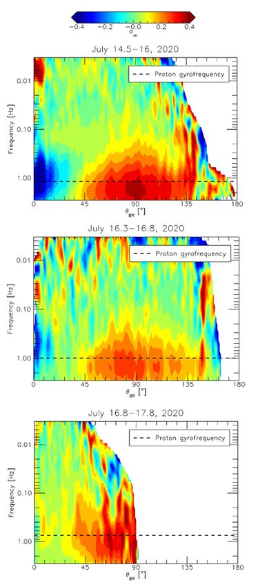
R. D’Amicis et al.: First Solar Orbiter observation of the Alfvénic slow wind and identification of its solar source

Panasenco & Velli (2013); Panasenco et al. (2019, 2020) such
regions may form easily when large scale pseudostreamers are
present in the corona. Pseudostreamers (PSs) are characterised
by multipolar regions of confined field, that open into interplane-
tary space in a unipolar fashion. Pseudostreamers therefore sep-
arate coronal holes with the same polarity, contrary to helmet
streamers (HSs) that form between coronal holes with oppo-
site polarities. The main differences between PSs and HSs are
1) the height of a pseudostreamer cusp or X-point is found to
be lower in the corona, by at least factor of 2, with respect to
the height of the Y-type neutral point of the HS tip (Wang et
al. 2012; Panasenco & Velli 2013); 2) the presence of a well-
developed current sheet above the HS tip and outward, but the
absence of an associated polarity reversal or current sheet in the
outer corona pseudostreamer; 3) the presence of at least two (and
possibly four, but always even-numbered) neutral lines at the
PS base, meaning that twin filaments may be harbored in PS
lobes. Field lines opening into space from the neighborhood of
pseudostreamer lobes tend to have non-monotonic, large expan-             Fig. 1. Position of Solar Orbiter during July 2020 (black dots). The plot
sions, as illustrated by coronal magnetic funnels in Panasenco            shows the projection of the orbit on the ecliptic plane in GSE (geocen-
et al. (2019), and the presence of filament channels in the pseu-         tric solar ecliptic) coordinates, so that Earth is at [0,0] (blue dot), the
dostreamer lobes increases the probability and strength of the            Sun is at [1,0] (yellow dot). Red dots highlight the position of the s/c
non-monotonic expansion and divergence of the open magnetic               during the selected interval.
field from pseudostreamer configurations in three-dimensional
modeling.
     The connections between the physical processes occurring at
the Sun and the features observed locally in the solar wind can           are jointly served by a data processing unit (SWA-DPU). This
now be studied thanks to the Solar Orbiter mission (Müller et             analysis, in particular, is based on solar wind measurements de-
al. 2020). Launched in February 2020, Solar Orbiter is a unique           rived from SWA-PAS which is an electrostatic analyser with a
mission to both study in detail the physics of the solar wind in          confined field of view (-24◦ to +42◦ × ±22.5◦ around the ex-
situ, thanks to four high-time-resolution instruments for plasma,         pected solar wind arrival direction). SWA-PAS measures the full
fields and energetic particles (Walsh et al. 2020), and its source        3D velocity distribution function (VDF) of the protons and al-
regions, through high-resolution remote-sensing observations by           pha particles arriving at the instrument in the energy range from
six different instruments (Auchère et al. 2020). Indeed, the com-         200 eV/q to 20 keV/e. From the VDF, ground moments (e.g.
bination of both in situ measurements and remote sensing ob-              number density, velocity vector and temperature computed from
servations (García Marirrodriga et al. 2021), for the first time in       the pressure tensor) are derived and provided at 4 sec resolution.
a single spacecraft in the inner heliosphere, will allow unprece-         The SWA-PAS database was downloaded from the AMDA web-
dented magnetic connectivity analysis between the solar atmo-             server1 . We also included magnetic field measurements from the
sphere and the inner heliosphere (Zouganelis et al. 2020).                Magnetometer (MAG) instrument (Horbury et al. 2020a), down-
     The Alfvénic slow solar wind is a statistically important solar      loaded from the ESA Solar Orbiter archive2 and averaged at the
wind regime, both in the inner heliosphere and at the Earth and           plasma sampling time.
in different phases of the solar cycle (D’Amicis et al. 2021a,b).
Although observed in previous missions, it is at present in the               Fig. 1 shows the projection of Solar Orbiter orbit, during July
limelight due to the very recent observations by Parker Solar             2020 (black dots), on the ecliptic plane. The plot is given in GSE
Probe, which observed several streams of Alfvénic slow wind               (geocentric solar ecliptic) coordinates, so that Earth is at [0,0]
at distance close to the Sun never reached before. The focus of           (blue dot) and the Sun is at [1,0] (yellow dot). The position of
this paper is the characterisation of an Alfvénic slow wind in-           the s/c in the period of our analysis is highlighted in red. Dur-
terval observed very recently by Solar Orbiter at about 0.64 AU.          ing that period, after its first perihelion on June 15, the s/c was
Data selection will be presented in Section 2. Section 3 will be          progressively moving away from the Sun.
devoted to a global description of the stream in situ character-
istics, while the connection between the in situ measurements
and the solar source will be discussed in Section 4. A summary
discussion of the results will be presented in Section 5.

                                                                          3. Global in situ description of the stream
2. Data selection
The study presented in this paper was performed over a time               Although the Alfvénic slow wind has mainly been observed and
interval ranging between 14 July 00:00 UT (universal time) to             studied during the maximum of the solar cycle, evidences of the
18 July 12:00 UT, 2020, during which Solar Orbiter crossed                presence of this solar wind regime occur also at the minimum of
an Alfvénic slow wind stream. A crucial set of measurements               the solar cycles (D’Amicis et al. 2021b). Indeed, Solar Orbiter
for our study is provided by the Solar Wind Analyser (SWA)                has been embedded in a stream of Alfvénic slow wind in July
suite of instruments (Owen et al. 2020), consisting of an Elec-           2020, during the minimum of solar cycle 24. In the following,
tron Analyser System (SWA-EAS), a Proton and Alpha Particle               we will give a complete description of this interval in terms of
Sensor (SWA-PAS), and a Heavy Ion Sensor (SWA-HIS) which                  Alfvénic content, plasma features and spectral properties.
                                                                                                                      Article number, page 3 of 16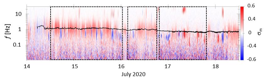
A&A proofs: manuscript no. output

                                                                                   The speed profile exhibits velocity variations of the order
                                                                              of ± 35-50 km/s, on typical timescales of 6-10 h, that can be
                                                                              attributed to the so called ‘microstreams’ as first observed by
                                                                              Ulysses in the fast polar wind (Neugebauer 1995, 1997) and
                                                                              in Helios data close to the Sun (Horbury et al. 2018). Neuge-
                                                                              bauer (2012) interpreted these structures as the in situ signature
                                                                              of reconnection jets, due to newly emerging bright-point loops
                                                                              with previously open magnetic fields (see e.g. Subramanian et
                                                                              al. 2010) present in the chromospheric network. Similar large-
                                                                              scale structures were observed also in the properties of the pro-
                                                                              ton plasma quantities and in the Alfvénicity (Borovsky 2016).
                                                                                   Following D’Amicis et al. (2021a) and references therein,
                                                                              we first study the Alfvénic content of the fluctuations. Alfvénic-
                                                                              ity can be studied using the Elsässer variables (Elsässer 1950),
                                                                              introduced for the first time in the interplanetary data analysis
                                                                              by Tu et al. (1989) and Grappin et al. (1991). The Elsässer vari-
                                                                              ables are defined as follows: z± = v ± b where b is the magnetic
                                                                              field expressed in Alfvén units (b = B/(4πρ)1/2 , with ρ being the
                                                                              mass density and B is the magnetic field). The sign in front of b
                                                                              is given by sign(−k · B0 ), where k is the wave vector and B0 is
                                                                              the ambient magnetic field:
                                                                               i) for a field directed outward with respect to the Sun, a nega-
                                                                                  tive (positive) correlation indicates a mode propagating away
                                                                                  from (toward) the Sun. In this case, Elsässer variables are de-
                                                                                  fined as z+ = v − b and z− = v + b for outward and inward
                                                                                  modes, respectively;
Fig. 2. Time series of plasma and other relevant parameters characteris-      ii) when the field is directed towards the Sun, the correlation
ing Alfvénicity in the slow wind stream observed by Solar Orbiter at a            sign reverses with respect to the previous cases. However, the
heliocentric distance of 0.64 AU: solar wind speed, V sw [km/s] (a); pro-         scientific community has agreed to define z+ (z− ) always as
ton number density, n p [cm−3 ] (black) and magnetic field magnitude, B           outward (inward)-directed Alfvénic fluctuations. To do this,
(red) (b); proton temperature, T p [K] (c); the normalised cross-helicity,        the magnetic field is rotated by 180◦ , every time that it is di-
σC (d); the Elsässer ratio, rE (e); the normalised residual energy, σR (f);       rected towards the Sun (Roberts et al. 1987; Bruno & Bavas-
and the Alfvén ratio, rA (g). The derived quantities are computed at 30
min scale.
                                                                                  sano 1991; Grappin et al. 1991). Then, in this case b → −b
                                                                                  and Elsässer variables are defined as z+ = v+b and z− = v−b.
                                                                              In this stream the magnetic field is essentially outward-directed
3.1. Alfvénic slow wind
                                                                              as we will see in the next section.
Fig. 2 shows an overview of the Alfvénic slow wind stream ob-                     In Fig. 2, as first introduced by Tu & Marsch (1995), we an-
served by Solar Orbiter at a heliocentric distance of 0.64 AU.                alyze the energy associated with z+ and z− modes, namely e+
The same time interval has been also studied in another paper                 (red) and e− (black) at 30 min scale as solar wind fluctuations
of this special issue by Louarn et al. (2021) focusing on differ-             show a strong Alfvénic character at this scale (Tu & Marsch
ent aspects and in particular on the characterisation of the proton           1995; Bavassano et al. 1998). In particular, we focus on their
distribution functions observed by PAS. During the selected in-               (normalised) difference, namely the normalised cross-helicity,
terval, the speed values (panel a) are less than 500 km/s thus                σc = (e+ − e− )/(e+ + e− ) (panel d), and their ratio, the Elsässer
identifying a slow stream. However, the speed profile is similar              ratio, rE = e− /e+ (panel e). As expected, there is a clear predom-
to that of a fast wind stream. Indeed, we observe a compres-                  inance of e+ respect to e− (σc close to 1 and rE  1) indicating a
sion region at the leading edge of the stream and a rarefaction               dominance of outward propagating Alfvén modes. Moreover, σc
at the trailing edge. The compression region (14.25 - 14.5 July)              profile evolves along the stream with higher values in the main
is characterised by an increase in the proton number density and              portion of the stream than in the rarefaction region. At the same
magnetic field magnitude (see panel b). The main portion of the               time, in the two regions, rE changes considerably with e+  e−
stream, extending from approximately 14.5 to 16 July, displays                in the main portion. On the other hand, we also evaluate the nor-
higher speed and large amplitude fluctuations and approximately               malised residual energy: σR = (ev − eb )/(ev + eb ) (panel f), and
constant n p and B. Then, a rarefaction region appears, which is              the Alfvén ratio, rA = ev /eb (panel g), where ev and eb are the
characterised by a gradual decrease of the flow speed and smaller             kinetic and magnetic energies, respectively. These quantities in-
amplitude fluctuations. Moreover, the proton temperature pro-                 dicate the imbalance between kinetic and magnetic energy of the
file, T p (panel c), follows the V-T relationship (see e.g. Burlaga           fluctuations. Fig. 2 shows overall an imbalance in favor of mag-
& Ogilvie 1970; Lopez & Freeman 1986; Matthaeus et al. 2006;                  netic energy (σR is negative implying eb > ev and rA < 1). Al-
Elliott et al. 2012; Perrone et al. 2019). This is indeed larger              though rA is very close to unity near the Sun (0.3 AU), it appre-
in the main portion of the stream than in the rarefaction region.             ciably decreases with increasing radial distance in near-ecliptic
The characterisation of the different portions of the stream will             solar wind (e.g. Bruno et al. 1985; Marsch & Tu 1990), reach-
be discussed in more details in the subsection 3.2.                           ing an asymptotic value of 0.5 around 1 AU. The departure from
                                                                              energy equipartition (namely eb ' ev as expected for an ideal
1
    http://amda.irap.omp.eu/                                                  Alfvén wave) might be due to the turbulence evolution (see e.g.
2
    http://soar.esac.esa.int/soar                                             Grappin et al. 1991; Roberts et al. 1992), to the effect of solar
Article number, page 4 of 16
R. D’Amicis et al.: First Solar Orbiter observation of the Alfvénic slow wind and identification of its solar source
divided by the product of their standard deviations:
P
j (V j − V̄)(B j − B̄)
ρvb = q (1)
2 2
P
j (V j − V̄) (B j − B̄)
where V j and B j are the velocity and magnetic field single mea-
surements and V̄ and B̄ are the velocity and magnetic field av-
erages in each 30 min window. In principle, this formula should
be applied to every component of the velocity (Vi ) and magnetic
fields (Bi ) (with i = R, T, N 3 ) and then we derive the total cor-
relation coefficient as the average from the three components,
i ρvbi /3. However, for the sake of simplicity, we consider only
P
the N component since more Alfvénic than the other two (Tu et
al. 1989). As in previous studies, ρvb indicates that the main por-
tion of the stream (red box of Fig. 4) is the most Alfvénic part
(very high absolute values of ρvb ), while Alfvénicity decreases
when moving towards the rarefaction region (blue box).
Fig. 3. 2D contour plot of σC vs σR for the Alfvénic slow wind stream The amplitude of velocity and magnetic fluctuations can
observed by Solar Orbiter at 0.64 AU. The color bar represents the per- be measured by their respective variances (panel c), defined as
centage with respect to the maximum value. Values of σC > 1 are arti-
σ2V = σ2VR + σ2VT + σ2VN (black) and σ2B = σ2BR + σ2BT + σ2BN (red),
facts of the 2D contour plot interpolation.
normalised to the square of their average fields. Both quantities
are larger in the main portion of the stream compared to the rar-
efaction region (blue box in Fig. 4), as also shown by Carnevale
wind structures (Tu & Marsch 1993) or also to effects related to et al. (2021). The higher variance of the fluctuations in the main
pressure anisotropy and ion differential streaming (Bavassano & portion indicates the presence of large amplitude Alfvénic fluc-
Bruno 2000). tuations. The transition between the main portion and the rar-
efaction region is such that the Alfvénic content of the fluctua-
The degree of the v-b correlation depends not only on the
tions along with the amplitude of fluctuations decrease consider-
type of wind, but also on the radial distance from the Sun and
ably (Ko et al. 2018).
on the time scale of the fluctuations (Bruno & Carbone 2013).
To understand the spatio-temporal evolution of the magnetic
Using 2D histograms of σC - σR (Bavassano et al. 1998), Bruno
field vector, we study the changes experienced by the vector ori-
et al. (2007) were able to characterise the turbulence state of so-
entation. Panel (d) displays the vector displacement, |δB|, be-
lar wind fluctuations of Helios observations and showed that at
tween each magnetic field instantaneous direction and an arbi-
short heliocentric distances (∼ 0.3AU) the turbulent population
trary fixed direction, normalised to the average magnetic field,
is largely dominated by Alfvénic fluctuations, characterised by
hBi, defined as:
high values σC and equipartition of energy. However, as the wind
expands, Alfvénic fluctuations are depleted and another popula- sX
tion, which displays lower values of σC and a clear imbalance |δB(t)|/hBi = (Bi (t) − Bi (t0 ))2 /hBi (2)
in favor of magnetic energy, becomes visible and easily distin- i
guishable from the Alfvénic population (Wicks et al. 2013). In
the top panel of Fig. 3, we characterise the state of turbulence of with i = R, T, N, as first studied by Bruno et al. (2004). The
this stream of Alfvénic slow wind in a similar way. A predom- arbitrary fixed direction was chosen to be the direction of the
inance of outward modes is observed, characterised by a mag- first vector of the time series, B(t0 ). However, the result of this
netic energy excess since the distribution extends over the quad- kind of analysis does not depend on this assumption. The vec-
rant σC > 0-σR < 0, in agreement with existing literature (Bruno tor displacement provides important information on solar wind
et al. 1985; Bavassano et al. 1998, 2000; D’Amicis et al. 2007, fluctuations, as shown in Bruno et al. (2004). Indeed, by look-
2011; D’Amicis and Bruno 2015). Moreover, the main feature ing how the magnetic field orientation fluctuates in space, these
is a pronounced peak corresponding to Alfvénic fluctuations (σc authors found that the magnetic fluctuations are characterised by
close to 1 and σR close to 0) and a tail towards lower values of the contribution of two components: small-amplitude and high-
σC , and more imbalanced magnetic structures (lower negative frequency fluctuations superimposed on a larger-amplitude low-
values of σR ) (Bavassano et al. 1998), features very similar to frequency background structure. Thus, this quantity is sensitive
the ones of the fast wind observed by Helios at 0.65 AU (Bruno to both propagating Alfvénic fluctuations and advected struc-
et al. 2007). tures (e.g., flux tubes), the two main ingredients of solar wind
turbulence (Bruno & Carbone 2013). Panel d clearly shows dif-
ferent regimes within the stream. Indeed, the main portion is
3.2. Identifying different portions of the stream dominated by directional fluctuations which are generally large,
i.e. the Alfvénic component. The other portions of the stream,
As anticipated in the previous subsection, different regions, with less (but still) Alfvénic, shows smaller fluctuations and fewer
well-defined features, can be identified in this Alfvénic slow large and quick directional jumps. This is in agreement with the
stream, as shown in Fig. 4. The solar wind speed is inserted in results by Bruno et al. (2004) and their interpretation according
panel (a) for completeness. Panel (b) shows the v-b correlation 3
Vi and Bi are in the heliographic Radial Tangential Normal (RTN)
coefficient, ρvb , computed at 30 min scale using a running win- coordinate system, where R points away from the Sun toward the space-
dow, as another parameter to measure Alfvénicity. It is defined craft, T is the cross product of the Sun’s spin axis and R, and N com-
as the ratio between the covariance of the two variables v and b, pletes the right-handed triad.
Article number, page 5 of 16A&A proofs: manuscript no. output
et al 2020; Mozer et al. 2020; McManus et al. 2020), naturally
associated with localised radial velocity enhancements (Kasper
et al. 2019; Horbury et al. 2020b) having oscillation amplitudes
comparable to the magnitude of the magnetic field (Bale et al.
2019). Although previously observed in the fast wind, by mis-
sions at different heliocentric distances (Behannon et al. 1981;
Tsurutani et al. 1994; Kahler et al. 1996; Balogh et al. 1999;
Yamauchi et al. 2002; Landi et al. 2006; Matteini et al. 2014;
Borovsky 2016), the switchbacks are ubiquitous features of the
Alfvénic slow wind in the inner heliosphere (e.g. D’Amicis et al.
2021a, and references therein).
The behaviour of the angle between the magnetic field and
the radial direction, θBR (panel f), provides similar information.
It shows large fluctuations around about 60◦ within the main por-
tion of the stream, while it is very small (almost radial field) in
the rarefaction region. This is a clear indication that, in the main
portion of the stream, the magnetic field direction is changing
due to the presence of large amplitude Alfvénic fluctuations.
Panel (g) shows the behaviour of the plasma beta, β, com-
puted as the ratio between the thermal pressure, pk and the mag-
netic pressure, pm or analogously as Vth2 /VA2 where, Vth , the ther-
mal speed, is defined as (2kB T p /m p )1/2 , and the VA , the Alfvén
speed, as B/(4πρ)1/2 , with kB the Bolzmann’s constant, T p the
average proton temperature, and m p the proton mass. The evo-
lution of β also identifies the different portion of plasma and, in
particular, it shows a transition from values higher than 1 in the
main portion of the stream to values well below 1 in the rarefac-
tion region.
It must be noted that the behaviour of the parameters charac-
terising the sub-interval (green box in Fig. 4) between the main
portion of the stream and the rarefaction region is rather differ-
ent from the other two. First of all, this interval is quite Alfvénic
but with smaller amplitude of the fluctuations with respect to
the main portion of the stream but larger than the rarefaction re-
Fig. 4. Time series of relevant parameters: solar wind speed, V sw [km/s] gion as shown in the behaviour of σ2V /hV 2 i and σ2B /hB2 i, and
(a); v-b correlation coefficient, ρvb (b), computed at 30 min scale (b); |δB(t)|/hBi. The radial component of the magnetic field does not
V and B variances normalised to the square of their respective mean
show switchbacks, rather a strong BR polarity inversion at odds
fields, σ2V /hV 2 i (black) and σ2B /hB2 i (red) (c); magnetic field vector dis-
placement, |δB|/hBi (d); radial component, BR [nT], in RTN coordinate with the dominant (positive) polarity of the stream. This reflects
system (e); angle between the magnetic field direction and the radial in a sudden change of θBR between very small values (almost
direction, θBR (f); and plasma beta, β (g). The red and blue boxes iden- aligned field) and θBR ∼ 120◦ . A detailed analysis of this region
tify the main portion of the stream and the rarefaction region, respec- will be performed in section 3.4. The difference in the switch-
tively. The green box identifies a region characterised by the presences back activity before 16 July 00:00 UT and after 16 July 18:00
of structures, that will be studied in detail in Section 3.4. UT, related to dramatic changes in the solar source region mag-
netic topology, will be discussed in Section 4.
To conclude this subsection, we analyzed the sharp discon-
to which the large jumps correspond to tangential discontinu- tinuity at day 16.766 (see Figure 2 and 4) which marks the be-
ities marking the borders between adjacent flux tubes. In each ginning of the rarefaction region and has been identified as a
flux tube the presence of Alfvénic fluctuations makes the mag- reconnection exhaust crossing. See also Lavraud et al. (2021),
netic field vector randomly wander about a local field direction. this special issue. This can be clearly seen in Figure 5, where
The effect of the directional jumps is to move the tip of the fluc- plasma and magnetic field observations are shown for the time
tuating vector from one particular average direction to another interval around the exhaust. Observations are reported in the
one (see also section 3.4 and Figure 10). LMN coordinates, with L (-0.81; -0.25;-0.52) being the direc-
The passage from one region to the other one is also marked tion of the anti-parallel component of the magnetic field (BL ),
by the different behaviour of the radial component, BR , of the M (0.31; -0.95; -0.022) the direction of X line (and of the guide
magnetic field (panel e), characterised by the presence of large field BM ) and N (-0.49; -0.18; 0.85) being along the normal to
and intermittent polarity reversals, called switchbacks, especially the current sheet. The N normal to the current sheet is computed
in the main portion of the stream. In the rarefaction region, the by means of the Minimum Variance (MV) analysis performed
field is almost radial in agreement with previous studies (e.g. across the exhaust (e.g. Sonnerup & Cahill 1967), M is com-
Orlove et al. 2013) and the switchback activity is much weaker puted as M = N × (BA − BB )/|BA − BB |, where BA and BB are
with much fewer inversions, and smaller amplitudes than the the magnetic field vectors tangential to the current sheet mea-
ones observed in the main portion of the stream. These polarity sured on the two sides of the exhaust, and L completes the or-
reversals, observed very recently by Parker Solar Probe, are S- thogonal triad (e.g. Davis et al. 2006). The plasma and field sig-
shaped magnetic structures (Dudok De Wit et al. 2020; Chhiber natures are characteristic of the crossing of a bifurcated current
Article number, page 6 of 16R. D’Amicis et al.: First Solar Orbiter observation of the Alfvénic slow wind and identification of its solar source
sheet encompassing decelerated plasma flows, which are roughly
Alfvénic, with the changes in V and B components (panels b
and d) being anticorrelated (correlated) on the leading (trailing)
portion of the exhaust. Moreover, such flows are quantitatively
consistent with the reconnection model that predicts that two ro-
tational discontinuities are present at the edge of the exhaust. In
such case, the plasma flows should vary across the current sheets
according to the relation:
h i1/2 h i
V pred = Vre f ± (1 − αre f )/(4πρre f ) (ρre f /ρ)B − Bre f (3)
where B, v, ρ are the magnetic field vector, plasma flow ve-
locity and mass density, respectively; Pk and P⊥ are the pres-
sure parallel and perpendicular to the magnetic field and α =
(Pk − P⊥ )4π/B2 is the pressure anisotropy factor (Hudson 1970;
Paschmann et al. 1970). The subscript ’ref’ indicates indicates
a dataset point in the ambient plasma in proximity of the dis-
continuity. In panels c and d of 5, the predicted values obtained
by the above relation are reported as black lines, with positive
(negative) sign for the trailing (leading) portion of the bifur-
cated current sheet and using for the leading (trailing) portion
the reference point indicated by the left (right) dashed line. The
leading and trailing portion predictions merge at about 16.778.
The comparison between the observed and predicted plasma
flows variations evidences that the observations are very well in
agreement with the quantitative prediction for reconnection. This
event would deserve a more detailed analysis that, however, falls
outside the scope of the present paper.
3.3. Spectral analysis
Fig. 5. From top to bottom: the magnetic field magnitude, B (panel a);
The identification of the different regions within the Alfvénic the magnetic field components in the LMN coordinates system (panel
slow stream also has implications on the spectral properties, that b); the solar wind speed, V sw (panel c); the solar wind velocity com-
motivated us to perform a comparative spectral analysis. ponents in the LMN coordinates system (panel d); the proton number
density, n p (e); and the proton temperature, T p (d). In panels c and d,
the black lines represent the reconnection model predictions according
3.3.1. Power spectra to Equation 3. The left (right) dashed line indicates the reference point
used for the prediction in the leading (trailing) portion of the exhaust.
The first part of the spectral analysis is devoted to a comparative
study of power spectra of the regions identified in Fig. 4, using
MAG data in normal mode with a sampling time of 0.125 s. Fig. the inertial and kinetic scales, as first identified by Bruno et al.
6 (bottom panel) shows the power spectral density (PSD) of the (2014) and more recently by D’Amicis et al. (2019).
trace of magnetic field fluctuations of the three regions. The PSD The upper panel of Fig. 6 shows the normalised power spec-
are computed over a one-day interval in the main portion of the tra of the trace of magnetic field fluctuations, similar to Bruno et
stream and in the rarefaction region (15 July 00:00-23.59 UT and al. (2019) and D’Amicis et al. (2020), to better highlight simi-
from 16 July 19:12 UT to 17 July 19:12 UT, respectively) and larities and/or differences between the relative amplitude of the
over 12 hours in the intermediate region (16 July 07:12-19:12 fluctuations and the scaling of the power spectra in the differ-
UT). The time resolution and the length of the interval allow us ent regimes we identified in this Alfvénic slow stream. The nor-
to clearly identify the three main frequency ranges of the turbu- malised power spectral density is derived in the following way.
lent spectrum, indicated in Fig. 6 as f −α , f −β , f −γ . Indeed, we The amplitude of the fluctuation δB( f ) at a given frequency f
observe an 1/ f scaling at low frequencies. Although its inter- can be computed as:
pretation has been highly debated (e.g. Matthaeus & Goldstein
δB( f ) = 2 f PB ( f )
p
1986; Dmitruk & Matthaeus 2007; Verdini et al. 2012; Tsurutani (4)
et al. 2018), it has been recently associated with the saturation of
the magnetic field fluctuations to the amplitude of the local mag- where PB ( f ) is the Fourier power spectral density. These values
netic field (Matteini et al. 2018; Bruno et al. 2019; D’Amicis et are then normalised to the corresponding local magnetic field in-
al. 2020; Perrone et al. 2020). Then, the inertial range is well- tensity averaged within each interval, hBi, so that the δB( f )/hBi
described by a spectral index between the Kraichnan and the is a dimensionless quantity that can be compared in different
Kolmogorov theoretical scaling. The higher power spectrum of solar wind regimes. According to the normalisation in Equa-
the main portion of the stream is the result of the presence of tion 4, the Kolmogorov scaling PB ( f ) ∼ f −5/3 corresponds to
large amplitude Alfvénic fluctuations characterising this region. δB( f ) ∼ f −1/3 , and the Kraichnan scaling PB ( f ) ∼ f −3/2 to
Finally, steeper spectra characterise the high frequency part of δB( f ) ∼ f −1/4 , indicated in the figure as dashed lines. The low-
the spectrum. In particular, the steepest spectrum corresponds frequency part of the spectrum shows a flattening corresponding
to the main portion of the stream characterised by the highest to the 1/ f scaling, indicating that the amplitude of the Fourier
power in the inertial range, highlighting a strong link between modes has saturated as discussed in Matteini et al. (2018) and
Article number, page 7 of 16A&A proofs: manuscript no. output
tended to wavelet analysis (e.g. Telloni et al. 2012), and further
refined to separate helicity contributions from different fluctua-
tions (Woodham et al. 2021). For this part of the analysis, we use
64 Hz burst-mode magnetic field measurements from the MAG
instrument, which has continuous coverage during our interval.
We calculate the normalised magnetic helicity in RTN coor-
dinates averaged over 1-min intervals:
n o
2= WT∗ (t, f ) WN (t, f )
σm (t, f ) = , (5)
|WR (t, f )|2 + |WT (t, f )|2 + |WN (t, f )|2
where Wi (t, f ) are the continuous Morlet wavelet transforms
(Torrence & Compo 1998) of the RTN magnetic field compo-
nents. This averaging procedure helps to smooth out some of the
variability in the full-resolution transform. We neglect the spec-
trum in that interval where a data gap is present within the corre-
sponding 1-min interval. σm takes values in the interval [−1, 1],
where σm = −1 indicates fluctuations with purely left-handed
helicity and σm = +1 purely right-handed helicity in the plasma
frame. A value of σm = 0 indicates no overall coherence.
In Figure 7, we plot σm (t, f ) for the interval 14.0-18.5 July.
In the spacecraft frame, the sign of σm depends on both the back-
ground field direction, B0 and the wave-vector k of the fluctua-
tions, which is Doppler shifted due to the Taylor hypothesis (e.g.
Woodham et al. 2019). Due to the small amplitude of the turbu-
lent fluctuations at small scales, the MAG noise floor can lead
to an artificial flattening of the power spectrum, at frequencies
above about 1 Hz in our interval. As the signal-to-noise ratio
decreases with increasing frequency, σm decreases towards zero
and so this signature is not real. We also see the presence of
right-handed fluctuations at frequencies, f > 10 Hz, which are
Fig. 6. Top panel: Normalised Power Spectral Density (PSD), δB/hBi, associated with an increase in power above the MAG noise floor.
derived as explained in the text, for the main portion of the stream (red), The Solar Orbiter Radio and Plasma Waves (RPW) (Maksimovic
for the rarefaction region (blue), and for the intermediate region (green). et al. 2020) observations by the search coil magnetometer are
The dashed lines correspond to the Kolmogorov scaling (δB( f ) ∼ f −1/3 ) able to properly characterise these wave modes, which have been
and to the Kraichnan scaling (δB( f ) ∼ f −1/4 ), along with a scaling
observed throughout the inner heliosphere (e.g. Lacombe et al.
δB( f ) ∼ f −5/4 corresponding to P( f ) ∼ f −7/2 , according to the normali-
sation described in the text. Bottom panel: PSD of the trace of magnetic 2014; Jagarlamudi et al. 2020). We do not address these signa-
field components for the three identified regions as in the top panel. The tures further in this paper.
slopes of the three frequency regimes are indicated with the same color Fig. 7 shows that coherent magnetic helicity signatures are
code of the different portions of the stream and are computed over the more prevalent in the main portion of the stream rather than in
following frequency ranges: f < 3 · 10−4 Hz, 2 · 10−3 < f < 10−1 Hz the intermediate region. Their occurrence rate in the rarefaction
and 2 · 10−1 < f < 2 Hz. region is even lower. The magnetic helicity signatures at pro-
ton scales in Figure 7 are consistent with many previous studies
throughout the heliosphere (He et al. 2011, 2012a,b; Podesta &
Bruno et al. (2019). The normalised PSD clearly shows that the Gary 2011; Klein et al. 2014; Bruno & Telloni 2015; Telloni et
three regions have different relative fluctuations, with the main al. 2015; Telloni & Bruno 2016; Telloni et al. 2019, 2020; Wood-
portion of the stream characterised by the largest relative fluctu- ham et al. 2019, 2021). The right-handed signature of σm ' 0.3
ations respect to the average background magnetic field than the centred at ∼ 1 Hz (close to the proton gyro-frequency, fcp , shown
other two regions. Indeed, the relative fluctuations decrease as as a solid black line in Fig. 7) is associated with right-handed tur-
one moves from the main portion to the rarefaction region, with bulent fluctuations propagating anti-sunward, with polarisation
the region characterised by the presence of the structures having properties consistent with KAWs (e.g., Howes & Quataert 2010;
an intermediate value. He et al. 2012b). The helicity signatures σm ' ±0.8 between 0.1-
1 Hz are associated with small-scale kinetic instabilities driven
3.3.2. Magnetic helicity spectrograms by non-equilibrium features in the particle distribution functions
(Kasper et al. 2002, 2008, 2013; Hellinger et al. 2006; Matteini
To better characterise the different portions of the stream, we et al. 2007; Bale et al. 2009; Maruca et al. 2012; Bourouaine
use a measure of the magnetic helicity, Hm , an invariant of et al. 2013; Gary et al. 2015; Alterman et al. 2018; Klein et al.
ideal magnetohydrodynamics (MHD), to analyze the nature of 2018, 2019).
the magnetic field fluctuations using their polarisation prop- The sign of the helicity is dependent on the direction of prop-
erties. Matthaeus et al. (1982) first introduced the fluctuating agation, which is not possible to determine due to the Doppler
reduced magnetic helicity for single-spacecraft observations, shift of proton distribution fucntions (Podesta & Gary 2011;
which gives the degree and handedness of helical rotations in B Woodham et al. 2019, 2021; Verniero et al. 2020; Bowen et al.
at a given frequency. More recently, this definition has been ex- 2020a; Bowen et al. 2020b). For an inward-oriented (negative
Article number, page 8 of 16R. D’Amicis et al.: First Solar Orbiter observation of the Alfvénic slow wind and identification of its solar source
Fig. 7. Spectrogram of the normalised magnetic helicity, σm . The dashed boxes are the same identified in Fig. 4. The black line corresponds to the
proton gyro-frequency.
polarity) magnetic field, assuming outward propagation, a left- Fig. 9 shows the time series of plasma and magnetic field
handed ion-cyclotron wave would have a positive magnetic he- parameters for this region: the solar wind speed, V sw (panel a);
licity and would correspond to a clockwise rotation of the mag- the normal, N, components of velocity, VN , and magnetic field
netic field vector. The same wave would result in negative he- in Alfvén units, VAN in RTN coordinate system (b); the proton
licity for an outward-oriented magnetic field (Narita et al. 2009; number density, n p (c), the proton temperature, T p (d), along
He et al. 2011). On the contrary, a right-handed kinetic Alfvén with magnetic field magnitude (e), azimuthal, ΦB (f) and polar
wave would have a negative magnetic helicity and would corre- angles, ΘB (g) and θBR (h). The bottom panels display kinetic, pk ,
spond to an anti-clockwise rotation of the magnetic field vector magnetic, pm and total pressure, ptot (i) and the plasma beta, β (l).
for an inward magnetic field and would have a positive magnetic These parameters allow us to identify different plasma parcels
helicity for an outward magnetic field. Hence, it is important to within the stream lasting typically around 30 minutes.
evaluate the angle θBR between the sampling direction assumed The last two structures at the end of the interval, highlighted
along the radial direction and the scale-dependent mean mag- with light red (labeled B0 ) and light blue (labeled R) boxes, re-
netic field. For this purpose, a complementary approach follows spectively, last longer. B0 and R are separated by the reconnec-
the angular distribution of the magnetic helicity. Based on Hor- tion exhaust crossing discussed in Sec. 3.2 event. The structure
bury et al. (2008), θBR between the local mean magnetic field and indicated as R has been already identified as the beginning of the
the sampling direction, is first computed as a function of t and rarefaction region. Although the magnetic field magnitude is al-
f . Then, σm (t, f ) is reordered into σm (θBR , f ), as first reported in most the same, B0 and R are oriented in two different directions
literature by Horbury et al. (2008); He et al. (2011); Podesta & (compare the magnetic field azimuthal and polar angles, ΦB and
Gary (2011) and later on by Bruno & Telloni (2015); Telloni et ΘB , and θBR in Table 1) and also the plasma parameters identify
al. (2015, 2020). For computational reasons, we use here normal different plasma parcels (notice the different but almost constant
mode MAG data at 16 Hz. values of n p and T p within the two structures). On the other hand,
The character of the fluctuations beyond the high-frequency the behaviour of the pressures is similar in the two cases, with a
break located between the fluid and kinetic regimes strongly de- similar behaviour for pk and pm , so that the plasma β is similar
pends on the Alfvénic content of the fluctuations in the iner- and smaller than 1. Not least, B0 is quite Alfvénic while in R the
tial range and on their amplitude (Telloni & Bruno 2016; Tel- v-b correlations are reduced (see also the behaviour of σc in Fig.
loni et al. 2019; Woodham et al. 2021). Similar to the fast wind 2 and of ρvb in Fig. 4).
(Bruno & Telloni 2015) and to a previous study on the Alfvénic Several structures at different scales are observed recalling
slow wind at 1 AU (Telloni et al. 2020), in the present study the spaghetti-like flux-tube texture of the interplanetary mag-
the main portion of the stream shows a clear signature of both netic field (McCracken & Ness 1966; Mariani et al. 1973;
right-handed and left-handed polarised fluctuations, around 90◦ Neugebauer 1981; Bruno et al. 2001; Borovsky 2008). The idea
and 0◦ , possibly associated with quasi-perpendicular KAWs and is that the s/c might cross the same structure during successive
quasi-parallel ICWs, respectively (see Fig. 8, upper panel). On time intervals. To prove this hypothesis, B0 along with the other
the other hand, the intermediate region and the rarefaction re- parcels identified as Bi (i = 1, 2, 3) were gathered in a group as
gion (intermediate and lower panel), where the wind speed and they display similar temporal evolution of different parameters.
the Alfvénicity of low-frequency fluctuations decrease, show a In a similar way, parcels labeled Ai were organized in a different
reduction in the presence of the ICW signature, in agreement group. In general, B structures show higher n p and lower T p val-
with Bruno & Telloni (2015). It is worth noticing that θBR in the ues than A structures. Moreover, Table 1 clearly shows that the
rarefaction region is limited to values smaller than 90◦ as also structures in each group have a different magnetic field orienta-
observed in Fig. 4. tion. In addition, most of the structures are quite Alfvénic (ex-
cept for the subinterval 16.5-16.6 comprising the magnetic dip
and other portions not highlighted in the boxes) and are gener-
3.4. Magnetic structures ally separated from one another by sharp discontinuities similar
to the tangential discontinuities already highlighted in previous
Fig. 4 clearly show that this stream can be divided in well- studies (e.g. Bruno et al. 2001). Indeed, along all the interval
defined regions, each one with peculiar characteristics. While the 16.2-16.9, there is no large variation of pressure values except
previous sections were devoted to a global comparative study of for the dip in the magnetic field around 16.5 that involves struc-
the three sub-intervals, in this section we focus on the charac- tures A1 , A2 and B1 . In this case, pk > pm thus resulting in a
terization of the region marked by a dashed green box in Fig. 4 β much greater than 1. A similar behaviour is observed in the
(16.2-16.9 July). reconnection event. In the rest of the interval pm > pk and β < 1.
Article number, page 9 of 16A&A proofs: manuscript no. output
Fig. 9. Time series of relevant parameters corresponding to the interval
16.2-16.8. From top to bottom: the solar wind speed, V sw (panel a); the
N components of velocity, VN , and magnetic field in Alfvén units, VAN
(b); the proton number density, n p (c), the proton temperature, T p (d),
along with magnetic field magnitude (e), azimuthal, ΦB (f) and polar
Fig. 8. Scalogram of the normalised magnetic helicity, σm (color map), angles, ΘB (g) and θBR (h); kinetic, pk , magnetic, pm and total pressure,
with respect to the angle, θBR , between the magnetic field and the radial ptot (i) and the plasma beta, β (j). The color boxes identify the structures
direction. From top to bottom: main portion of the stream, intermediate which have been grouped in structures A and B, along with the begin-
region and rarefaction region. The dashed line in each plot corresponds ning of the rarefaction region identified as R. All the structures have
to the proton gyrofrequency in the s/c frame. been identified with grey boxes apart from R in light blue and B0 and
B2 with light red as explained in the text.
In particular, β ∼ 0.7, before the dip, while β is close to 0.5 after
the dip. means of the angle the MV forms with the average magnetic field
A MV analysis further reveals the intrinsic similarities and (θB−MV ) and with the radial direction (θR−MV ). Table 1 contains
differences of the two groups and of the rarefaction region. The a summary of the MV variance analysis performed over all the
maximum, intermediate and minimum eingenvalues of the MV structures labeled Ai and Bi and also on R. From the comparison
matrix are identified as λmax , λint , λmin respectively. In all cases, of magnetic field orientation and of the MV results, we can eas-
λmin
λmax , λint thus clearly identifying the MV direction by ily exclude B1 from ‘group B’. Actually, although the magnetic
Article number, page 10 of 16You can also read