Improvement of the Cheetah Locomotion Control - (BioRob)/EPFL
←
→
Page content transcription
If your browser does not render page correctly, please read the page content below
É COLE P OLYTECHNIQUE F ÉDÉRALE DE L AUSANNE
P ROJET DE M ASTER
2010
S ECTION DE M ICROTECHNIQUE
TULEU Alexandre

                               Master Project Report
               Improvement of the Cheetah
                  Locomotion Control.

  Professor : Auke Jan I JSPEERT
  Supervisor : Alexander S PROEWITZ
  Date : January 29, 2010 Edited version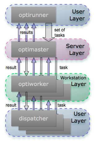
Abstract

     This project relates to the locomotion of Cheetah , a small and light robot, who features tri-
segmented, biologically inspired, compliant legs. It is a continuation of former BIRG students
projects, who brought the conception of two simulated model and two prototypes.
     This project focuses on the simulation aspect, where a Central Pattern Generator (CPG) is used
to abstract the control of the locomotion, and evolutionary algorithms are used to perform offline
learning with a model of the robot in the W EBOTS simulator.

     At first, the model of the robot has been improved to be more accurate toward the prototypes,
particularly on the level of the asymmetric compliant behavior of the leg. Afterwards the control
software has been carried out with the use of new Optimization and CPG framework developed at
BIRG . Then an implementation of locomotion self-stabilization principles, observed in quadrupedal
locomotion, has been introduced inside a Central Pattern Generator previously designed by Ludovic
R IGHETTI. Finally, the extensive study of a learned trot gait has been completed, measuring the
benefit of the implementation of such behaviors.
Contents
Introduction 3
1 Presentations and Motivations 4
1.1 Locomotion behavior in Nature for inspiration . . . . . . . . . . . . . . . . . . . . 4
1.1.1 Similarities in locomotion between quadruped mammals. . . . . . . . . . . 4
1.1.2 Leg retraction as a Self-Stabilization leg control strategy . . . . . . . . . . 5
1.1.3 Central Pattern Generators : a model for animal locomotion control . . . . 6
1.2 Cheetah a compliant leg robot . . . . . . . . . . . . . . . . . . . . . . . . . . . . 7
1.2.1 Global presentation of the Cheetah . . . . . . . . . . . . . . . . . . . . . 7
1.2.2 Asymmetric compliance leg design . . . . . . . . . . . . . . . . . . . . . 7
1.2.3 Previous simulation model of Cheetah . . . . . . . . . . . . . . . . . . . 8
1.3 Goals of the project . . . . . . . . . . . . . . . . . . . . . . . . . . . . . . . . . . 9
2 Modelization of Cheetah in W EBOTS 10
2.1 Knee Articulation Modelization . . . . . . . . . . . . . . . . . . . . . . . . . . . 10
2.1.1 Modelization of the cable . . . . . . . . . . . . . . . . . . . . . . . . . . . 11
2.1.2 Servo Specifications . . . . . . . . . . . . . . . . . . . . . . . . . . . . . 12
2.1.3 Implementation in W EBOTS . . . . . . . . . . . . . . . . . . . . . . . . . 13
2.1.4 ODE unrealistic behavior with the Cheetah knee mechanism . . . . . . . . 16
2.2 Using the B IO ROB Software framework. . . . . . . . . . . . . . . . . . . . . . . . 19
2.2.1 LIBCPG - NETWORK an Object Oriented simulator of dynamical system. . . 19
2.2.2 Optimization framework . . . . . . . . . . . . . . . . . . . . . . . . . . . 19
2.2.3 Extension of the job file . . . . . . . . . . . . . . . . . . . . . . . . . . . 20
2.3 Software organization . . . . . . . . . . . . . . . . . . . . . . . . . . . . . . . . . 22
2.3.1 General . . . . . . . . . . . . . . . . . . . . . . . . . . . . . . . . . . . . 22
2.3.2 Cheetah Controller . . . . . . . . . . . . . . . . . . . . . . . . . . . . . . 22
2.3.3 Physics Plug-in . . . . . . . . . . . . . . . . . . . . . . . . . . . . . . . . 24
2.3.4 WorldMaker . . . . . . . . . . . . . . . . . . . . . . . . . . . . . . . . . 25
3 Implementation of the locomotion control 26
3.1 Central Pattern Generator defintion and extension . . . . . . . . . . . . . . . . . . 26
3.1.1 A Central Pattern Generator for quadrupedal walking . . . . . . . . . . . . 26
3.1.2 Addition of the leg retraction principle . . . . . . . . . . . . . . . . . . . . 30
3.2 Definition of the offline learning process. . . . . . . . . . . . . . . . . . . . . . . 32
3.2.1 Particle Swarm Optimization . . . . . . . . . . . . . . . . . . . . . . . . . 32
3.2.2 Fitness Evaluation definition. . . . . . . . . . . . . . . . . . . . . . . . . . 32
3.2.3 Choice of the Open Parameters . . . . . . . . . . . . . . . . . . . . . . . . 33
4 Execution of the learning process 35
4.1 PSO parameter tuning . . . . . . . . . . . . . . . . . . . . . . . . . . . . . . . . . 35
4.1.1 Clamp and Zero invalidation mode comparison . . . . . . . . . . . . . . . 35
4.1.2 Use of a decreasing constriction to increase the exploration of the parameter
space . . . . . . . . . . . . . . . . . . . . . . . . . . . . . . . . . . . . . 36
4.2 Study of a learned trot gait without sensory feedback . . . . . . . . . . . . . . . . 38
14.2.1 Dynamical analysis . . . . . . . . . . . . . . . . . . . . . . . . . . . . . . 38
4.2.2 Proposition of a method to find the less influential parameters . . . . . . . 41
4.2.3 Insight for improving the gaits . . . . . . . . . . . . . . . . . . . . . . . . 43
Conclusion 44
Bibliography 3
Glossary 5
Acronyms 7
List of Figures 8
List of Tables 9
2Introduction
In recent years, there are more and more designed robot, which are biomomimetics copies of
animals, like for example the Sony Aibo entertainment robot. But bioinspired robotics is not just
making robot that look like animals, it is understanding the underlying principle of the animal, and
adapt them to machine [WHI+ 00].
Cheetah is a robot that try to follow this idea : it features compliant, pantographic leg, that are
designed from observations in small mammals [WHI+ 00, FB06]. In addition, previous work on this
robot [Rie08, Kvi09], used Central Pattern Generator (CPG) to control its locomotion : they are a
model of how animals produce rhythmic neural activities to control their movements. CPG abstract
the command of the whole dynamic, with a few parameters. One approach is to use optimization
algorithms to learn the optimal value of these parameters, to perform locomotion.
The same approach is taken in this project. After a in-depth presentation of Cheetah and
locomotion behaviors in nature, an improvement of the simulated model of Cheetah is presented.
Then an extension of an existing CPG is proposed. Finally the study of a learned trot gait with the
work flow is carried out.
[Med]
3Part 1
Presentations and Motivations
Legged locomotion is a well spread mechanism in nature. However, due to the complex mech-
anisms it implies, (complex movement of limbs, complex bodies dynamics, non continuous contact
with the ground, ...), it is also one of the most challenging problem in robotics. A way to outcome
these difficulties, as stated by [WHI+ 00] is to take inspiration from the nature, as the behavior found
in animal, results from evolution process of thousands of generations.
Cheetah is an implementation of this idea. Thus, to understand its conception choice, locomo-
tion behavior found in quadruped mammals will be introduced before the presentation of the actual
robot and the previous work about this platform. Finally the goal of this project will be introduce.
1.1 Locomotion behavior in Nature for inspiration
As it names let it guess, Cheetah takes inspiration from the mammals. After a brief presen-
tation of behavior and "blueprints" found in mammals, it will present how locomotion control is
abstracted with Central Pattern Generator (CPG).
1.1.1 Similarities in locomotion between quadruped mammals.
Study of the animal locomotion behavior is a growing field in biomechanics [Ale84, FSS+ 02,
FB06, WBH+ 02, Sch05]. As stated by [WHI+ 00], the extension of the biomechanics to the animal
yield to the extraction of principles that could extend the engineer toolbox. As the common ancestor,
in an evolution point of view, of large quadruped and biped mammals like horse, dog and humans
are the small mammals, the study should focus in first place on the later.
[FB06, WHI+ 00, WBH+ 02], compares and extract several similarities between several species,
that are useful to understand why animal are so efficient in locomotion.
- The limb of mammals are almost Tri-segmented shaped (see figure 1.1), and have the same
forelimb and hindlimb configuration in term of functionality [FB06]. However the serial
segments are no longer homologous.
- The progression is mainly due to the retraction - caudal displacement of the limb - of the most
proximal segment i.e., the scapula for forelimb and the femur for the hindlimb, [FB06].
- Two segments (scapula/lower arm for forelimb and femur/foot) operate almost parallel during
retraction of the limb, as in a pantograph mechanism, [FB06, WHI+ 00].
- High limb compliance is a general principle for small mammals, and this help the self-
stabilization of the limb, i.e., the stable locomotion of the animal, in presence of external
disturbance without the necessity of a sensory feedback, [FB06], More details are given in
the section 1.1.2
- In asymmetrical running gait, like galop, canter, or bound, the animals extensively use the
bending of their spinal cord, and thus the back of the spine become the main propulsive
segment for the hindlimb [FB06, WHI+ 00].
4Figure 1.1 – The tri-segmented limb abstraction for small mammals. If the most distal segment are omitted,
the limbs are segmented in three parts : (a) for the forelimbs : scapula, humerus and lower arm, (b) for the
hindlimbs : femur, shank and foot . Taken from [FB06].
- One can observes in certain animals, a connection between the wrist and precedent segment.
This connection is made by elastic tendons, which also gives compliant foot/hand.
One of the most important point before, is the self-stabilization capacity of the leg in animals.
Indeed, if the robot dynamics, passively goes into a limit cycle, it simplifies its control effort [IP04].
Therefore one might be interested in other self-stabilization behaviors.
1.1.2 Leg retraction as a Self-Stabilization leg control strategy
As stated previously, the self-stabilization of the locomotion seems to be a general strategy
among the animals. At least three self-stabilization principle has been observed :
1. leg stiffening : animals can modulates the leg stiffness to perform different gait, and also
stabilize it [DK09]. However it is too difficult to implement such a mechanical behavior for
a light robot, so this possibility has not been investigated further.
2. leg extension : it has been shown for small birds, that at each stride, the leg is automatically
fully extended if the contact on the ground has not been made at the expected touchdown. This
behavior limit the changes of height of the Center of Mass (CoM), under ground height dis-
turbance like step up and step down, which help the self-stabilization of the animal [DVB09].
However as this is not a well known behavior for quadruped locomotion, it had not been
investigated further.
3. leg retraction : that state the animal start the retraction of the limb a certain time before the
touchdown. Then the foot touches the ground with a non-zero horizontal velocity [SGH03].
To bring out this last behavior [SGH03] uses a spring mass model, where the angle of attack is
controled. This model although it is conservative, is asymptotically stable, and predict human data
at moderate running speed. However it was not stable for low speed, and a high accuracy of the
angle of attack is needed to achieve stability.
5Figure 1.2 – Leg retraction principle for [SGH03]. The angle at APEX and the rotational velocity are controlled,
which provides an increase of the basin of attraction of the global system according to [SGH03].
[SGH03] extend this model : instead of controlling the angle of attack at each touchdown,
controls the angle at the APEX - point where the height of the Center of Mass (CoM) is maximal
- and the rotational velocity of the leg, once the APEX is passed (see figure 1.2) . Thus it showed
that the bigger this speed is, the more it increase the size of the basin of attraction of the system.
Moreover this model is also able to find limit cycle for low speed running gait.
1.1.3 Central Pattern Generators : a model for animal locomotion control
Central Pattern Generators are now a well diffused assumptions in biologically fields, as stated
in [Ijs08], that movement in animals are centrally generated through block of neurons, that generate
rhythmic pattern of neural activity, without receiving rhythmic input.
They are a big field in biologically research, and it has been established several neurobiological
models, at different levels. All these models are good tools for describing the movements, and
there is more and more research over the past few year, that try to use this model to control the
locomotion of robots. [Ijs08] propose several reasons for preferring the use of a CPG instead of
classical methods :
1. The purpose of CPG models is to exhibit limit cycle behavior, therefore they are more robust
to perturbation.
2. CPG models have only few parameters to drive speed, direction or even the type of gait.
Therefore, at higher level, the command is simplified, as command just have to provide only
a small number of variable.
3. CPG are ideally suited for sensory feedback, that able us to control finely the mutual interac-
tion between the CPG and the body dynamics.
4. CPG are a really good substrate for learning and optimization algorithm.
They are several model of CPG that are well suited for robotics control from standard to
modular robot, like phase oscillator [IC07, SMM+ 08] or Hopf modified oscillators [RI08, Wie08].
It is the last one that is used in Cheetah . Note, as an analogy with biological study, the oscillators
are also named neurons, as in biological fields, these oscillators are just a mathematical macroscopic
model of how a group of neurons acts.
6Figure 1.3 – First prototype of the Cheetah robot.
1.2 Cheetah a compliant leg robot
1.2.1 Global presentation of the Cheetah
[WHI+ 00] propose several principles for the design of bioinspired quadruped robots. These
principles has been partially applied by [Rut08] in the design of the Cheetah robot. The first proto-
type is then a small and light robot, who has a size similar to a small cat. It features tri-segmented
pantographic leg, which are compliant, and actuated by two Degree of Freedom (DoF), in the hip
and in the knee. In agreements with [WHI+ 00], all its actuators are located on the main part, the
trunk, and the actuation of the knee is made through Bowden cables (section 1.2.2).
1.2.2 Asymmetric compliance leg design
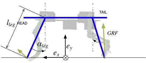
The legs of Cheetah are tri-segmented; They are designed with a pantographic mechanism
(see figure 1.4) such as the femur (l3 ) and the foot (l1 ) are always parallel. The kinematic may be
abstracted by the leg segments (λ1 , λ2 , λ3 ). [Rut08] proposed the following relative length (1.1) for
one leg, and a total leg length of 150 mm for the forelimb and 180 mm for the hindlimb.
λ3 = 0.39
λ2 = 0.45
(1.1)
λ1 = 0.16
λ p = 12mm
Figure 1.4 – Schematics of the Cheetah robot, from [Rut08]
7(a) Resting position (b) Actuated (c) Under external forces
Figure 1.5 – Passive functioning of the compliant mechanism of the pantographic leg of the Cheetah . Here,
for drawing simplification, the actual Bowden cable is replaced by a simple wire.
The compliance of the leg is within the knee mechanism. As shown in figure 1.5, the motor is
pulling a Bowden cable that tends to reduce the diagonal of the parallelogram of the tibia segment,
and then contract the leg. One can sees three operation modes :
1. If there is no action of the servo, and no action on the distal segment, then the spring extends
the leg at its maximum (figure 1.5a).
2. If the motor pulls the wire, then it contract actively the leg (figure 1.5b).
3. In the presence of external interaction (if the robot stands on the ground), then the wire
is loosened, disconnecting the motor from the system. The equilibrium is obtained by the
spring, counter-acting the gravity force from the weight of the robot.
[Rut08] state that this leg can be abstracted by a single compliant leg, with the use of the
following equation for the leg length and angle :
q
lλ = Lλl = λ22 sin2 ϕ + (λ1 + λ3 − λ2 cos(ϕ))2 (1.2)
λ1 + λ3 − λ2 .cos(ϕ)
cos(ϕ3 − αleg ) = (1.3)
λl
1.2.3 Previous simulation model of Cheetah
In order to study the locomotion of the Cheetah , a W EBOTS model of the robot had been made
by Yvan B OURQUIN and Martin R IESS [Rie08] (see figure 1.6a). The purpose was to use this model
and implement a Central Pattern Generator designed by Ludovic R IGHETTI (see [RI08] and section
3.1), thus a quantitative study of a couple of gait (walk and trot) have been done. The approach
used by [Rie08] was to use a mechanical model really close to the reality. However the model was
complex, causing large computation time. Thus it prevents the use of optimization algorithm, which
large amount of trial for the optimization of one gait.
Then another study had been made by Ivan K VIATKEVITCH [Kvi09] (see figure 1.6b), with
a more abstracted model of the leg. This new model did not perform sufficiently, so it had been
decided to use a more reality-close one. However [Kvi09] pointed out some flaw in the W EBOTS
simulation like the bad quality of contact modelization and the need to filter the sensory feedback
information
8(a) Realistic model by Martin R IESS (b) Abstracted Model by Ivan K VIATKEVITCH
Figure 1.6 – The two previous models of Cheetah in W EBOTS
1.3 Goals of the project
1. Recover and update the previous work on the cheetah platform :
• Choose among the previous W EBOTS model made by [Rie08] and [Kvi09].
• Create new foot with just a straight segment, connected with a rotational spring (stiff-
ness is to determine ).
• optionally :
– Make the geometry of the model as a parameter for optimization.
– Add a new DoF for each legs (hips).
– Add a spine to the robot. Look in the literature for possible spines.
• Assure the model is sufficiently coherent with the reality, by making him carrying
weight, drop it on the ground, and some naive gaits.
2. Prepare the optimization process by using the Optimization framework made by Jesse VAN
DEN K IEBOOM . It should be extended for using any optimization algorithm wanted, or type
of Central Pattern Generator (CPG).
3. Use the CPG, as described by Ludovic R IGHETTI [RI08]. The foot trajectory should be
generated, using two principles found in animal legged locomotion. This could be done by
either inverse kinematics or integrated in the CPG. The leg retraction behavior should also be
carried out and tested .
4. Make extensive research on :
• search for a good fitness function that does take into account control of speed, gait and
direction changes (with the emphasis on speed and robustness).
• the stability of the walk, by examining some criteria as Zero moment Point or Pointcaré
return map. This information could be also use to increase the basin of attraction of the
locomotion, by using it in the CPG.
• study the robustness of cheetah under terrain changes of slope (up, down, tilt right and
left), and changes of friction.
• the optimal leg geometry (optional).
9Part 2
Modelization of Cheetah in W EBOTS
The first task to this project was to choose between Martin R IESS or Ivan K VIATKEVITCH
model. As the introduction of Jesse Optimization framework helped to distribute evolutionary al-
gorithms over cluster of computer, speed is not the first priority. Therefore the more realistic Model
has been chosen.
At first some minor changes had been done on the model :
1. The legs were redesigned to have both a functional length of 160 mm ( see section 1.2.2).
2. The legs have now the same cranial orientation (first segment femur/scapula is oriented to-
ward the head). Previously the forelimb had their femur caudally oriented.
3. The density of the materials has been updated.
4. The weight of the servo-motor has been updated due to a change of type between the first and
second prototype of Cheetah .
However the biggest changes were maid for the Knee actuator. Indeed the original model were
biased. The system described in 1.2.2 was indeed modelized by a linear motor with a P Controller.
Thus the asymmetrical behavior was obtained by the fact that in one direction the maximum force
available is different from the other. This is not the case in reality, as the motors see a non-constant
non-linear charge. Thus a better modelization of the servo-motor had been developed.
2.1 Knee Articulation Modelization
The Cheetah robot knee actuator present an asymmetry (section 1.2.2) and then cannot be
straight forward modelized in W EBOTS using only W EBOTS primitives. Therefore a mathematical
model of the mechanism must be created, who features a more precise model of the servo-motor,
whose characteristic had been guessed.
Figure 2.1 – Mechanism of the knee actuator.
10τ pert
Umot KI τmot + τch 1 Θmot µred Θout
+ R+L.p + 0 ).p2
(Jeq
− ηred
Ωmot
Ke .p
Figure 2.2 – Model of the servo-motor.
The knee mechanism is show in figure 2.1. He is comprised of a servo-motor (α, τ) that drive a
wheel, on which is fixed a cable with a spring. The movement of the cable ∆xc can also be different
from ∆x. One can found the following relation :
∆xc = α.R (2.1)
where τc is the couple from the cable tension, and R the ratio of the gear :
τc = r.Fc (2.2)
and where Fc is the cable tension. For the servo-motor, the following model is used as described
by figure 2.2. The following notation is used :
• KI and KE respectively the torque and speed constant of the DC motor.
• R and L respectively the intern resistance and inductance of the DC motor
• Jeq the equivalent inertia of the motor axis with its charge.
• µred and νred , respectively the efficiency and the ratio of the gear.
It results the following 2nd order equation that drives the motor :
µred µ2
Jeq Rα̈(t) + KE KI α̇(t) = KI U(t) − red
2
Rτc (t) (2.3)
ηred ηred
Finally, it is assumed that the motor is controlled by a PID controller (however, one must notice
that the constructor could have settled a more sophisticated controller) :
Z t
U(t) = k p (αdes (t) − α(t)) + kd (α̇des (t) − α̇(t)) + ki (αdes (t) − α(t)) dt (2.4)
0
2.1.1 Modelization of the cable
Their are two ways to modelize the cable : by a spring or a rigid body.
2.1.1.a Asymmetric Spring Model
The cable tension is defined by using the equation of a spring with a constant kc >> ks . Then
the value of Fc is given by equation (2.5) :
(
kc (∆xc − ∆x) ,if ∆xc ≥ ∆x
Fc = (2.5)
0 , else
112.1.1.b Asymmetric rigid body
In the case of a pure rigid cable, then the value of Fc can be computed as the solution of an
optimization problem :
αr ≤ x
α̇r ≤ ẋ , i f
αr = x
min (Fc ) , with : (2.6)
Fc
equation(2.3)
Fc ≥ 0
Equation (2.3) show us that Fc is a decreasing function of (α, α̇, α̈). One can compute Fc using
the algorithm 1.
Algorithm 1 Computation of the tension of the rigid Bowden cable
1: procedure COMPUTE T ENSION I N R IGID C ASE(x(t), ẋ(t), α(t), α̇(t), α̈(t))
2: if α(t).r ≥ x(t) then . We violate our first boundary condition
x(t)
3: αN = r . We decrease α in order to respect our first condition
αN −α(t)
4: α̇N = dt + α̇(t) . We compute the corresponding speed
5: if α̇N > ẋ then . We don’t respect the second condition
6: ȧl phaNN = ẋr . decrease speed in order to respect second condition
7: α̈NN = α̇NNdt−α̇ + α̈ . Compute corresponding acceleration
8: αNN = (α̇NN − α̇) .dt + α . Compute corresponding position, we have αNN < αN ,
so first condition is still valid
9: . Now as we have the "should be" state, we compute Fc using equation (2.4)
U = k p (αdes− αNN ) + kd . (α̇des − α̇NN ) + ki . 0t (αdes (t) − αNN
R
10: (t)) dt
2
ηred µred
11: return max µ 2 .R η .KI .U − Jeq .Rα̈NN − KE .KI α̇NN , 0 . We make sure we
red red
have the last condition full-filled
12: end if
13: α̈N = α̇Ndt−α̇ + α̈
14: . Now as we have the "should be" state, we compute Fc using equation (2.4)
U = k p (αdes− αN ) + kd . (α̇des − α̇N ) + ki . 0t (αdes (t) − αN(t)) dt
R
15:
η2
16: return max µ 2red.R ηµred .KI .U − Jeq .Rα̈N − KE .KI α̇N , 0 . We make sure we have
red red
the last condition full-filled
17: end if
18: return 0 . here the cable is loosened
19: end procedure
2.1.2 Servo Specifications
This new mathematical model is based on lot of the mechanical characteristics of the servo-
motor, like the gear ratio and efficiency, motor inner characteristics ... However these characteristics
are not given for almost all servo-motor, and particularly for the one used by Cheetah (DYNAMIXEL
RX-28). Therefore these parameters have to be estimated from the few characteristic given by the
constructor (see table 2.1) : as the gear ratio of the servo is given, one can estimate some of the
characteristics of the motor.
As the mark and series of the motor, the motor with the closest characteristics can be found in
the constructor documentation [Mot], ( table 2.2).
For the gear, it seems that DYNAMIXEL use a custom one. So the value of a Maxon gear that
could be fitted in the servo-motor is taken. Its specifications are given by table 2.3.
12Type Constructor Data Estimated value for the motor
Gear ratio 1:193 -
Weight 72 g < 72 g
Applied Voltage 12 V 12 V
2,781
Stall Torque 2, 78 Nm 193 = 14, 04 mNm
Maximum velocity with no load 59, 9 rpm 59, 9 ∗ 193 = 11560 rpm
Starting Current 1, 2 A 1, 15 A
Mark and series of the motor Maxon ReMax Series Maxon ReMax Series
Table 2.1 – Dynamixel RX-28 constructor specifications, from [Rob], and estimated value for its DC motor.
The weight and starting current are smaller, as one must take into account the weight of the additional gear and
packaging, and the current consumption of the electronic command.
Characteristic Value
Nominal Voltage 12 V
No load Speed 11500 rpm
Stall torque 14, 4 mN.m
Starting Current 1, 45 A
Internal resistance 8Ω
Torque Constant 9, 32e−3 N.m.A− 1
Speed Constant 9, 92e−3 V.s.rad− 1
Weight 26 g
Rotor Inertia 0, 868 g.cm2
Table 2.2 – Specification of the Maxon ReMax 21 48 97, from [Mot]
Characteristic Value
Ratio 1 : 199
Inertia 8e−3 g.cm2
Efficiency 0, 53
Weight 30 g
Table 2.3 – Guessed specification for the gear, from [Mot]
2.1.2.a Tuning of the PID parameter
Once the characteristic are chosen, the last step is to find the good parameter for the PID
constant. For that purpose the Ziegler-Nichols closed loop method [Wik] is applied on the model
of one motor. Ziegler-Nichols is applied on the servo-motor alone because the end-user of the
servo-motor doesn’t have access to the tuning of the controller.
The ultimate gain obtened is KU = 1870 with oscillations of period TU = 72 ms. Therefore the
value of the PID are given in table 2.4 for the PID.
kp kd ki
KU .0, 6 = 1123 k p T8U = 10, 09 TU
2k p = 0, 025
Table 2.4 – PID parameter identified by Ziegler-Nichols closed loop method
2.1.3 Implementation in W EBOTS
2.1.3.a Implementation using a force driven linear servo-motor
The following system has been firstly implemented on W EBOTS , using a linear W EBOTS
actuator to model the global system composed of the servo, the spring (with mechanical stops) and
the cable. This servo is directly commanded by the force computed by the new model.The two
13cable model described in section 2.1.1 are implemented, but only the spring one currently stable.
The following algorithm is used to update the state of the system :
1. Get the value xt from W EBOTS , and compute ẋt
2. Retrieve previously computed αt , α̇t , α̈t .
3. Compute Fct using one of the two model described in section 2.1.1.
4. Compute Fout , the actual force to add in W EBOTS , by adding it the spring force and a damping
force.
5. Derive the W EBOTS linear servo-motor with the computed force Fout
6. Update αt+1 , α̇t+1 , α̈t+1 using equation (2.3) and a Runge-Kutta 4 method (instead of a Euler
one to avoid computation instability).
In order to prevent some instability in the model, the following limitations had been added :
- The order given to the servo are prefiltered, not to exceed maximum speed the servo can give
(Vmax = 6, 27 rad.s−1 ). It is done by a low-pass filter (see algorithm 2)
- The cable tension is limited to an amount Fcmax = 45 N with the spring cable model.
- A damping value of 60 Nm−1 s has been added on the spring. This value had been empirically
computed to reduce oscillation of the spring.
Algorithm 2 Low pass filter on command.
t , α t−1 )
procedure LOW PASS F ILTERO N C OMMAND(αdes des
t −α t−1
αdes des
if dt > Vmax then
t −α t−1
αdes
des
dt t−1
return .Vmax + αdes
α −α t−1
t
des des
dt
else
t
return αdes
end if
end procedure
2.1.3.b Comportment under extreme conditions
A minimalist simulation has been computed, where the four knee actuators had a command that
was over the speed limit the servo can admit, in order to see the model consistency. The results are
made of a movie of the simulation (http://akay.fr/data/CheetahHardCondition.
avi) and the output measured from W EBOTS (see figure 2.3)
This figure shows the following results :
• The servo-motor doesn’t see any load, because desired and real angular position concord.
Indeed all the charge is taken by the springy cable.
• There is an expected mismatch between desired and observed contraction in absence of dis-
turbance, because of the use of a spring cable.
• The cable force is noisy, as oscillations of high frequencies appear, but it is asymptotically
stable.
14Figure 2.3 – Output of a knee actuator (with a springy cable) at the limit of its capacities. One can sees that :
(a) the desired servo position match the computed output. This is less due to the well tuning of PID parameters,
than the fact that the cable (because it’s a spring) is taking all the load (b) the spring movement is noisy, with
high frequency oscillations. However, its seems asymptotically stable. (c) the final contraction of the spring
is always lower than the desired one, in absence of disturbance. It is not surprising due to the springy cable.
However the compliance of the leg appears when the leg touches the ground.
However this last point brings up some problems : These high oscillations make the model
overcome overriding mechanical stop constraint. Under a high disturbance the tibia segments could
go over their end positions and become crossed each other. Such a problem appears because these
constraints are too soft. Open Dynamics Engine (ODE), the physics engine upon which W EBOTS
is based, permits the tuning of the softness of these constraints through the tuning of the Constraint
Force Mixing (CFM)/Error Reduction Parameter (ERP) parameters.
An empirical tuning of these parameters was performed, in order to avoid such a situation.
However this brought another problem as it will be discussed in section 2.1.4.
2.1.3.c Discussion and further improvement
Although this method works to implement the symmetric behavior of the leg, some further
improvements are needed :
• The first annoying thing, is that the servo doesn’t see any charge, so a workaround must be
found.
• The hard cable model is not working, because, in opposition with the spring mode, it sends
all the load of the mechanism to the servo-motor, causing too high torques on the servo-motor
axis, and then causing numerical explosion of the model.
• Under high constraint, the W EBOTS joints of the mechanism are oscillating around their axis,
due to the high constraints of the mechanism. One way to deal with is to tune more finely the
ERP / CFM parameters for these particular joints, but it is not an easy job to do in W EBOTS ,
because this must be done inside a physics plug-in (W EBOTS only let use manage ERP and
CFM on a global perspective).
• The spring constant is limited to an amount of 3000 N.m−1 , to preserve consistancy of the
mechanism simulation. Although the prototype had lower value (≈ 2300 N.m−1 ) this is a low
value compared to the one Martin R IESS used (5000 N.m−1 )
15One way to deal with all of these problems would be to reduce the time step of the simulation.
There is not so many scopes for this, because the current time step is already small (4 ms). One
way too deal with the first two problems alone, is to only decrease the time step of the integration
of the model, by repeating step 3,4 and 6 of the algorithm (section 2.1.3.a) several times for each
simulation step. However this possibility has not been yet tested.
2.1.4 ODE unrealistic behavior with the Cheetah knee mechanism
2.1.4.a Problem description
As described by figure 2.4, the model of the Cheetah was subjected to unrealistic behavior :
the complete robot was not able to fall on the side, or more precisely, takes several minute to roll of
a few degrees.
(a) t = 0 s (b) t = 30 s (c) t = 60 s
Figure 2.4 – ODE physics simulation unrealistic behavior. Although Cheetah should fall on the side in a short
time, it takes minute to do so.
Yvan B OURQUIN, who design in first place the model under W EBOTS , observed this behavior,
by increasing the CFM parameter. However :
• A good tradeoff between the resolution of this problem and the stability of the new knee
actuator model was not found.
• It is pretty hard for a human observer, to determine the correctness of the simulation, without
a pretty good analytical model of the system, or real data to compare with the numerical
model, And at the time of this project, none of both was available, and then it is hard to find
the correct value for the CFM.
Therefore, it might be useful to present the meaning in ODE of these parameters.
2.1.4.b Presentation of the ERP/CFM parameters
Open Dynamics Engine is the physics engine used by W EBOTS [Cyb], and like almost physics
engine, it is based on the integration of the 2nd Newton law for rigid bodies [ODE]. The con-
tact forces and joint constraint forces (forces that maintain the restriction of motions between two
bodies) are expressed by ODE - and other - as a solution of a linear optimization problem under
constraint, in a similar way than for the rigid Bowden cable constraint in section 2.1.1.b.
A choice made by ODE, is the possibility to transgress this constraint, in order to gain some
computation time. Other physics engines that use hard constraint resolution like A RBORIS [ISI],
are much slower in comparison.
There are two parameters that drive how the constraints are managed [ODE] :
• Error Reduction Parameter : it is a value between 0 and 1. it drives the forces that are added
to bodies,in order to align correctly, those which joint position have drifted apart due to
numerical instability. 0 mean that the bodies can drift apart (no extra forces will be applied),
and 1 means that the solver will try to correct the numerical drift in one single step. A value
between 0.2 and 0.8 is advised by [ODE].
16• Constraint Force Mixing : it is a value > 0 that indicates how much the solver can violate
a constraint, by in some way, reducing proportionally to the CFM value the forces resulting
from a given constraint.
Then, in addition to reduce the computation time, these parameters could be used for the
experienced user to modelize soft constraints. But a bad tuning could also lead to instabilities.
Therefore one can imagine, the fact that the increase of CFM solves the unrealistic behavior, is
because the system is over-constrained. However it is a bad approach to release these superfluous
constraints by increasing CFM :
• It denotes more a problem of conception of the ODE model, and the fault should rather be
searched here.
• Under big external disturbances, the use of a high CFM also lead to unrealistic behavior of
the legs (section 2.1.3.b)
• Closed loop must be carefully performed. If there is some initial misplacement of the bodies
axis, it will cause unrealistic torque and force to be added, to maintain the constraints. And
as the goal is to modify the model programmatically, usually it may have such errors.
Therefore, in this project it will be better to find out the constraint, that cause these unrealistic
behavior.
2.1.4.c Finding the design problem of the model
(a) t = 0 s (b) t = 90 s (c) t = 360 s
(d) t = 0 s (e) t = 0.5 s (f) t = 1 s
Figure 2.5 – Test of two closed loop mechanism similar to the Cheetah ’s leg mechanism. With only one
closed loop (no closure between the piston and the ankle), the simulation seems to be physically realistic.
W EBOTS comes with several samples of a closed loop mechanism, and several come with more
than two loops. All simulations seemed realistic, and used a standard CFM parameter. However
None used closed loop that recovers each other, i.e. where several joints of the two loops have the
same axis.
So a small model was made in W EBOTS , that is exactly the same mechanism of the Cheetah
leg but with easily computable dimensions (a square mechanism, angle of 90 and 45 degrees) to
avoid bad closure of the loop. All joints were tuned to be passives, to reduce the error of a bad
command, and the loop closure was made by the same code than for the Cheetah legs. It leads to
17the following results : in the presence of a double intersected loop closure, the same bug appear in
huge proportions.
It seems to be a restriction of ODE not to be able to solve such mechanisms. But as the
resolution of this problem is part of the ODE internal, the easier solution is to open one of the two
loop of the mechanism.
2.1.4.d Resolution of the design error
As the model of the knee actuator directly give us the output force of the system (composed of
the spring, the Bowden cable, and the servo-motor), it is easiest to remove the closed loop between
the "muscle" part and the ankle joint (see figure 2.6). Then, to drive the whole mechanism, the
physics plug-in is used, to tell ODE to apply directly the computed force from the knee model,
between the femur and foot bodies, aligned on the diagonal of the mechanism (figure 2.6b).
(a) 2 loop (b) 1 loop
Figure 2.6 – Old and new mechanical model of the leg in W EBOTS . To avoid the unrealistic behavior,
the second closed loop is opened, and the forces computed with the model are directly applied to mechanical
bodies in the physics plug-in. The other part are conserved and are driven by servo to follow their real position,
to keep the accuracy of the Cheetah limb inertia.
However the knee model needs the contraction of the spring as input (section 2.1.3). For this
purpose, a direct kinematic model of the leg is used. This model is also used to drive the W EBOTS
servo-motors of the "muscle" part, in order to follow the position these bodies should have, in the
case where the 2nd loop is closed.
One can notice that these parts aren’t anymore useful for the modelization of the knee, and are
only kept to maintain the accuracy of the leg inertia computation. If one want to neglect this inertia,
these parts should be removed from the model.
182.2 Using the B IO ROB Software framework.
The second task of the project was, to include the B IO ROB 1 Software framework made by
Jesse VAN DEN K IEBOOM [vdK09], to control, and perform offline learning of the Cheetah. What
is presented here is just a brief overview, for a more in depth presentation please refer to the corre-
sponding documentation .
After the presentation of the two main tool of this framework, an overview of the whole con-
troller will be done.
2.2.1 LIBCPG - NETWORK an Object Oriented simulator of dynamical sys-
tem.
The first software is the LIBCPG . As seen in section 1.1.3, CPG are often referred as dynamical
system, and more precisely, as a network of coupled oscillators.
The LIBCPG has been conceived like a general, Object Oriented simulator for dynamical sys-
tem, and is not limited to the only study of CPG : the user defines objects that contains properties,
that are mathematical expression that can reference other properties of the same object. Data can
be transmitted between object with the use of link. Some property can be marked as "integrated",
in order to establish differential equation of 1st order for this property. Then by combining dif-
ferent object property and link, one can simulate any dynamical system with an Euler integration
principle.
The library permits the definition of such dynamical system, in several way :
1. Directly with the C API.
2. Through the definition of an XML file that defines the dynamical system. It is then loaded
and executed in a program with the C API.
3. With the use of a GUI, that help the creation and debugging of the XML file.
This library features also a way to make controller that easily drive a W EBOTS model with
a CPG, as a property of an object could be automatically linked to a command value of a Servo
in W EBOTS . However as in this case, the output values doesn’t drive directly W EBOTS servo-
motor, but complex model are used that seems hard to code using the LIBCPG , one couldn’t use
this feature. But for this purpose, two tools are proposed (section 2.3.2), and a extension of the file
job description (section 2.2.3), to facilitate the creation of generic controllers.
2.2.2 Optimization framework
As stated by its name, the purpose of this framework is to solve optimization task. but more-
over, it is designed to distribute all the computation in parallel on several computer. Indeed this
framework only implement evolutionary algorithms. All of these algorithms have in common to
maintain a set of solutions where their fitness are estimated at each iteration. Therefore the paral-
lelization of the algorithm is straight forward, as these estimations are independent from each other.
When performing offline learning of a robot, this lead to huge decrease of the computation time
: the fitness computation of one individual is time consuming as it is often the estimation of the
behavior of a simulated robot for a certain duration.
This framework gives all the tools necessary to perform optimization on several computers.
Moreover, a cluster of 45 computers is maintained at B IO ROB , in addition of a token server to share
fairly the available computational power over several end users. Each components is dedicated to
one particular task :
1 new name of BIRG
19Figure 2.7 – Overview of the optimization framework. End user had to step in the optirunner program through
an XML job definition file, and in writing the right dispatcher program for its application.
• The OPTIRUNNER program, which is used by the end user to launch optimization task, defined
by an XML job file.
• The OPTIMASTER program, which is run on a server. Each OPTIRUNNER that are performing
optimization are connected to it, and send it tasks. Then the OPTIMASTER distribute them to
available workstation.
• Each workstation are running OPTIWORKER programs. They are connected to the OPTIMAS -
TER and receive one task description at a time. Then OPTIWORKER prepare the environment
and launches the DISPATCHER .
• A DISPATCHER program is responsible of the computation of a task. In evolutionary algo-
rithms, it is the fitness computation of an individual. Then it send back the result to the
OPTIWORKER , who will transmit it to the OPTIMASTER and finally the later will give back
the result to the OPTIRUNNER .
The end user had to :
• manage the OPTIRUNNER program, by providing the job definition file, that define the type
of optimization algorithm and it settings, the parameters to optimize with their boundaries,
and which dispatcher to use.
• provide the right dispatcher that will perform a given task.
Here a W EBOTS DISPATCHER is used, that load simulation of Cheetah . The robot is driven by
a CPG as described in section 3.1 and implemented with the LIBCPG . However if a small changes
is made to the optimization process, like the parameter to explore, the W EBOTS controller might
also need some small changes which is cumbersome. So an extension of the job configuration file
structure is proposed.
2.2.3 Extension of the job file
The goal of this extension, is to made the controller aware of which optimization parameter
and settings are linked to which CPG parameter.
For this purpose the definition of the parameter node of the job description file is extended
[vdK09] from :
20to :
...
where object_name and property_name designate the property of one object, the pa-
rameter parameter_name is linked to.
The possibility to link LIBCPG properties to setting is also added by adding the
node after the one :
...
...
...
and then each defined under whose name is setting_name
will be linked to the corresponding LIBCPG properties.
212.3 Software organization
2.3.1 General
The software that controls the optimization of the Cheetah relies on three main parts, a W E -
BOTS controller a physics plug-in, and the WORLD M AKER executable.
For the W EBOTS controller the goal was to develop a generic controller for the Cheetah , where
everything is controlled by configuration files. With this approach, several optimizations could be
performed in the same time. This would not be possible, or easily manageable, if the executable
needs to be recompiled, at each change of parameter.
The role of the WORLD M AKER is to programmatically change the geometric configuration of
the Cheetah .
The whole software was coded in C++, because it is an industry standard Object Oriented
language. For complex task like GUI, the Q T library has been used, which is an open source library
under LGPL license. However the whole framework can be at runtime independent from Q T and
can be used without it (with the absence of a GUI, for example during optimization). However all
the Makefile generation is handled by the QMAKE utility which is part of the Q T development tool.
2.3.2 Cheetah Controller
The controller can be launched in two mode :
• OPTIMIZATION mode : it act as a back end for a . It can
perform different types of optimization through the use of .
• RUN mode, when compiled with Q T libraries : it launches a GUI that controls for example
the properties, or monitors some values of the robot.
The launch of the controller need some arguments :
• -j/-job (mandatory) : path to the XML job configuration file
• -c/-cpg (mandatory) : path to the XML cpg configuration file
• -o/-optimization : launches the controller in optimization mode (will try to get a
request from a dispatcher, if none will quit)
• -r/-redirect : will redirect stdout (standard output) on a temporary unique file
• -n/-none : will launch the controller in VOID mode, all actuator will stay at their zero
position.
While performing OPTIMIZATION mode, the controller can use the additional dispatcher
settings :
• "Simulation::Duration" : who in most cases defines the duration of the estimation
of one individual. It depends of the used (section 2.3.2.a).
• "ValidityTest" which is a string of the form :
Test1:Args11:Args12:....|Test2:Arg21:Arg22:...|.....
where "TestX" designate a (section 2.3.2.b), and "ArgsXY" its
arguments. The number of arguments depend on the «> ValidityTest>
• "OptimizationType" which designate the to use.
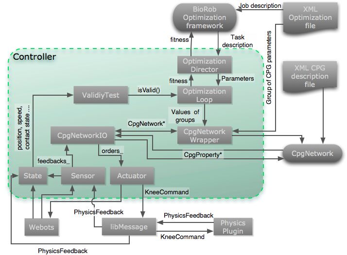
22Figure 2.8 – General organization of the controller.
2.3.2.a and classes
An is responsible for providing the loop of a certain type of opti-
mization, and for defining what will be the response of the task. The
take charge of getting the task description from the dispatcher, and of selecting the right Optimiza-
tionLoop.
The also check the validity of the Cheetah , through
the . If the state become invalid, the simulation is stopped, and the corre-
sponding fitness is returned without any further computation.
Currently two are implemented :
• : the simulation will last for "Simulation::Duration" time.
then the traveled distance along the x direction (clamped to a minimum of zero) is returned.
The corresponding value of "OptimizationType" is "distance" , and its the default
value.
• : the simulation is run several time, with a user defined parameter
being changed. Then the weighted mean (weight are also defined by the user) of the fitnesses
is returned. The corresponding value of "OptimizationType" is "uniform" .
2.3.2.b class
The tests if the of the Cheetah is valid through the use of
. The enabling/disabling and configuration of is done
with the "ValidityTest" setting. There are several ValidityTest implemented know :
• : tests if the speed over the last second of the cheetah is too high. Its setting
name is "Speed" and it takes one numerical arguments.
• : tests if the distance traveled by the robot is too high. Its setting name
is "Distance" and it takes one numerical arguments.
23• : tests if the geometric center of Cheetah is outside defined bounds. Its
setting name is "Height" and it takes two numerical arguments. First argument is the
upper bound and second the lower.
π
• : tests if the robot had a pitch or roll rotation of more than 2 from its
starting position. Its setting name is "Renversed" and it takes no argument.
• : test if the trunk of the Cheetah is touching the ground. Its setting name
is "Contact" and it takes no argument.
2.3.2.c and
These two classes are respectively abstraction of the actuator output and sensor input of Chee-
tah . permits the implementation of more complex model then P controlled
. There are several implemented :
• is the same as a .
• free joint. Used to measure the corresponding joint angle.
• modelize the knee actuator as in section 2.1.
• modelize the toe actuator as a passive spring.
There is two implemented classes. Both of them use basic signal processing on
the W EBOTS data. The signal is filtered by a low pass filter, and hysteresis threshold. Then
they both return value that are either 0.0 (no contact) or 1.0 (contact).
1. that use a standard as input for the
signal.
2. that use direct measurement of the Ground Reaction Forces
(GRFs) from the Physics plug-in.
2.3.2.d and
The class aims to manage the input and output of the
. Then it gives the orders to the and receives feedback from the .
The is responsible for extracting the parameters of the job file
that are associated with properties. Then it give an interface to easily access
these properties.
2.3.3 Physics Plug-in
The physics plug-in is a dynamic library that is responsible for :
• Closing the mechanical loop of the leg at the ODE world initialization.
• Apply the forces computed from the model (section 2) and given by .
• extracting, at the end of each step, the GRFs, and send them back to .
• detecting if the trunk of the Cheetah is in contact with the ground and send back the informa-
tion to the Controller
• Display visual hints, like the knee forces, and the Ground reaction forces.
• Enable and disable a , that restrict the motion of the Cheetah to the sagital
plane.
For the communication with the controller, the previously developed library LIB M ESSAGE
was used [Tul09, May09].
242.3.4 WorldMaker
The WORLD M AKER is responsible for the automatic generation of W EBOTS model of the
Cheetah with the use of the "worldBuilderPath" . This option of optimization feature permits
to test different leg configuration.
The WORLD M AKER can be launched from the command line with the -i/-interactif
option. Then it will ask for the value that define the leg configuration.
If no option are specified, it will follow the expected comportment of WORLF B UILDER : it
will
• read the standard input for a ,
• generate the world file in a unique-named, temporary file,
• send back the location of this file on standard output.
In this mode, the job description file must also provide the additional dispatcher settings :
• "Cheetah::Fore::LegDescription" , a string that describe the geometry of the fore-
limbs , which is of the form "Length|FemurCoeff|TibiaCoeff|FootCoeff|DeltaTibia"
, where :
– "Length" is the total length of the leg.
– "FemurCoeff" is the λ3 parameter of figure 1.4.
– "TibiaCoeff" is the λ2 parameter of figure 1.4.
– "FootCoeff" is the λ1 parameter of figure 1.4.
– "DeltaTibia" is the λ p parameter of figure 1.4.
• "Cheetah::Hind::LegDescription" the same parameters as the previous one, but
for hindlimbs.
• "Cheetah::Controller::Arguments" , which is the standard arguments to pass to
the Cheetah controller.
The WORLD M AKER has been made upon the LIBWBT , a library who add be designed for the
writting of W EBOTS world file (.wbt).
25Part 3
Implementation of the locomotion
control
3.1 Central Pattern Generator defintion and extension
For the control of the Cheetah a Central Pattern Generator, previously designed by Ludovic
Righetti[RI08] has been used. This CPG is able to generate up to four gait found in quadrupedal
(walk, trot, pace and bound), and features sensory feedback, that synchronizes the command with
the state of the foot (stance and swing phases). After a presentation of this CPG, a modification is
proposed to introduce the leg retraction strategy.
3.1.1 A Central Pattern Generator for quadrupedal walking
3.1.1.a General presentation
The CPG proposed by [RI08], is based on a modified Hopf oscillator. There are four neurons
which have a state (xi , yi )
ẋi = α(µ − r2 )xi − ωi yi (3.1)
ẏi = β (µ − r2 )yi + ωi xi + ∑ ki j y j (3.2)
j6=i
ωst ωsw
ωi = + (3.3)
1 + eby 1 + e−by
According to [RI08], this oscillator exhibit a limit cycle (see figure 3.1) , which is the circle of
√
radius µ in the phase space (x, y). [RI08] shows that the choose of the appropriate coupling matrix
(ki, j ) for four oscillators, leads them to phase lock. The resulting difference of phase between the
oscillator depends on symmetries between block of the chosen matrix (see figure 3.2 as an example).
[RI08] also gives 4 matrices for each of the following gait : walk, trot pace and bound.
Figure 3.1 – Representation of the attraction field of one oscillator. from [RI08]
26Figure 3.2 – Trot coupling for the CPG. taken from [RI08]
One nice property of this oscillator, is that the phase velocity ωi is not constant, but is "smoothly"
separated into two phases :
• the stance phase for y < 0. In this case the ωst term is prevailing in (3.3).
• the swing phase for y > 0. In this case the ωsw term is prevailing in (3.3).
However this introduces some drawback. One can remark experimentally, that even the aver-
age of the two angular frequencies ωst and ωsw is kept constant, it doesn’t set the frequency of the
final system. Indeed the relation between angular frequency and the frequency f of the limit cycle
is not straight forward : if the system (3.1-3.3) is transformed in polar coordinates (r, θ ), T = 1f
becomes the result of the following integral :
Z 2π
1 1
=T = ω ω√sw dθ (3.4)
f 0 √st +
1+eb µ sin(θ ) 1+e−b µ sin(θ )
Which is not easily computable.
This have two consequences :
• the angular frequencies should be the same for each of our oscillators : oscillator with differ-
ent frequency will converge slower (or even not converge) to a global limit cycle. The final
frequency is also not easily predictable.
• It is hard to relate the duty factor expected for one leg, to the value of the angular frequency.
An approximation of the integral (3.4) is proposed, in order to relate the duty factor to the
angular frequencies and frequency.
3.1.1.b Relations between frequency, angular frequencies and duty ratio
The idea behind the equation (3.3) is to use the hyperbolic tangent to "smoothly" switch be-
tween the two angular frequencies. Then for high values of b, the switch is almost instantaneous
between the two values. In the other case for small values of b, the value of ω is almost constant.
For this two cases, the expressions of the angular frequencies depending on the main frequency
of the oscillator and its duty ratio is presented :
- Case b >> 1 In this case, the integral (3.4) is divided in two parts :
Z 2π
1 1
Z π
T= ω ω√sw dθ + ω ω√sw dθ
0 √st + π √st +
1+eb µ sin(θ ) 1+e−b µ sin(θ ) 1+eb µ sin(θ ) 1+e−b µ sin(θ )
| {z } | {z }
= ω1sw = ω1
st
(3.5)
π π
= +
ωsw ωst
ωst + ωsw
T =π
ωst ωsw
27One can also identify in (3.5) the half period corresponding to stance phase Tst = ωπst and the
half period corresponding to the swing phase Tsw = ωπsw . Therefore the definition of the duty ratio d
becomes :
Tst ωsw
d= = (3.6)
T ωsw + ωst
This bring up the expressions of the angular frequencies depending on f and d :
π
ωst = f (3.7)
d
π
ωsw = f (3.8)
1−d
- case b• Have a fast transition between the two phases of the oscillator:
– while the oscillator is in the stance phase, and the foot leaves the ground.
– while the oscillator is in the swing phase, and the foot touches the ground.
• Stop the transition of the oscillator :
– from stance to swing phase, while there is still a sufficient weight supported by the foot.
– from swing to stance phase, while the foot still doesn’t touch the ground.
For this purpose [RI08] propose to add the following control input ui to equation (3.2) :
− sign(yi )F for fast transition
ui = − ωi xi − ∑ ki, j y j for stop transition
(3.12)
j6=i
0 otherwise
The sensory feedback should either not be enabled for every time. [RI08] propose to activate
the sensory feedback only for subspace of the phase space ( see figure 3.3)
3.1.1.d Use with Cheetah
For controlling the Cheetah , this CPG is used. However, with some trial test it appears that the
global dynamical system converge much faster with the same µ for the four oscillators. Therefore,
the possibility to have different value for the front and hindlimb is important, the following values
are added for the command.
ϕihip = ai ∗ xi + hi (3.13)
ȧi = ka ai − ades
i (3.14)
ḣi = kh hi − hdes
i (3.15)
Where ai is the the amplitude of the oscillator and hi its offset. The two last equation provide only
smooth changes of these parameters, the user should only change the values ades i and hdes
i
Figure 3.4 – Threshold for extension/contraction of the knee joint.Θextension and Θcontraction defines the two
regions where the leg should be either contracted (ϕiknee = λi > 0) or extended (ϕiknee = 0).
There are two active joints per leg. As stated before, the most proximal joint (here the hip
joint) must brought the most considerable contribution to the locomotion [FB06]. So ϕi becomes
output as the command of the hip joint. The knee joint, according to the principle of [WHI+ 00], as
the most active distal joint must only drives the foot clearance. Therefore the joint must only jump
from the state "extended" ( ϕiknee = 0 ) in the stance phase to the state "contracted" (ϕiknee = λi ) in
the swing phase. This behavior is parameterized by two thresholds (figure 3.4) :
(
knee 0 if Θextension ≤ θi < Θcontraction
ϕi = (3.16)
λi else
29You can also read