(In)Stability for the Blockchain: Deleveraging Spirals and Stablecoin Attacks
←
→
Page content transcription
If your browser does not render page correctly, please read the page content below
(In)Stability for the Blockchain: Deleveraging Spirals and
                                                                 Stablecoin Attacks∗
                                                                   Ariah Klages-Mundt†                 Andreea Minca‡
arXiv:1906.02152v2 [q-fin.TR] 4 Jun 2020

                                                                                    June 5, 2020
                                                                             Original release: June 2019

                                                                                          Abstract
                                                     We develop a model of stable assets, including noncustodial stablecoins backed by cryp-
                                                 tocurrencies. Such stablecoins are popular methods for bootstrapping price stability within
                                                 public blockchain settings. We derive fundamental results about dynamics and liquidity
                                                 in stablecoin markets, demonstrate that these markets face deleveraging feedback effects
                                                 that cause illiquidity during crises and exacerbate collateral drawdown, and characterize
                                                 stable dynamics of the system under particular conditions. From these insights, we sug-
                                                 gest design improvements that aim to improve long-term stability. We also introduce new
                                                 attacks that exploit arbitrage-like opportunities around stablecoin liquidations. Using our
                                                 model, we demonstrate that these can be profitable. These attacks may induce volatility
                                                 in the ‘stable’ asset and cause perverse incentives for miners, posing risks to blockchain
                                                 consensus.

                                           1     Introduction
                                           In 2009, Bitcoin [19] introduced a new notion of decentralized cryptocurrency and trustless
                                           transaction processing. This is facilitated by blockchain, which introduced a new way for mis-
                                           trusting agents to cooperate without trusted third parties. This was followed by Ethereum [22],
                                           which introduced generalized scripting functionality, allowing ‘smart contracts’ that execute al-
                                           gorithmically in a verifiable and somewhat trustless manner. Cryptocurrencies promise notions
                                           of cryptographic security, privacy, incentive alignment, digital usability, and open accessibility
                                           while removing most facets of counterparty risk. However, as these cryptocurrencies are, by
                                           their nature, unbacked by governments or physical assets, and the technology is quite new and
                                           developing, their prices are subject to wild volatility, which affects their usability.
                                               A stablecoin is a cryptocurrency with an economic structure built on top of blockchain
                                           that aims to stabilize the purchasing power of the coin. A true stablecoin, often referred to as
                                           the “Holy Grail of crypto”, would offer the benefits of cryptocurrencies without the unusable
                                           volatility and remains elusive. A more tangible goal is to design a stablecoin that maximizes
                                           the probability of remaining stable long-term. If one can establish guarantees for the stability
                                           of such a stablecoin, this would be a significant step toward forming a robust decentralized
                                           financial system and facilitating economic adoption of cryptocurrencies.
                                              ∗ We thank David Easley, Steffen Schuldenzucker, Christopher Chen, Sergey Ivliev, Tomasz Stanczak, and

                                           Sid Shekhar for helpful discussions. All errors are our own. AK and AM are funded through NSF CAREER
                                           award #1653354. AK thanks Lykke, Binance, and Amherst College for additional financial support.
                                              † Cornell University, Center for Applied Mathematics
                                              ‡ Cornell University, Operations Research & Information Engineering

                                                                                              1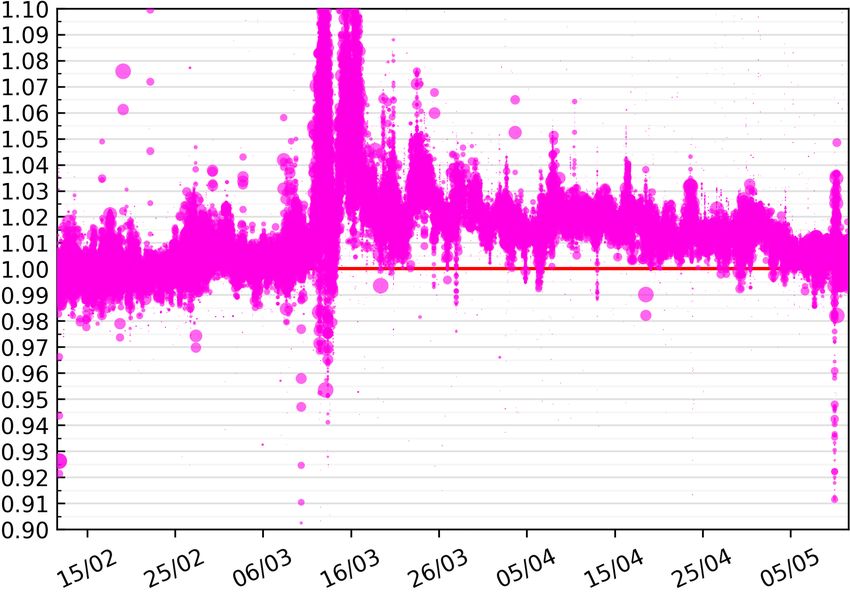
Cryptocurrency volatility Cryptocurrencies face difficult technological, usability, and reg-
ulatory challenges to be successful long-term. Many cryptocurrency systems develop different
approaches to solving these problems. Even assuming the space is long-term successful, there
is large uncertainty about the long-term value of individual systems.
    The value of these systems depends on network effects: value changes in a nonlinear way as
new participants join. In concrete terms, the more people who use the system, the more likely
it can be used to fulfill a given real world transaction. The success of a cryptocurrency relies
on a mass of agents–e.g., consumers, businesses, and/or financial institutions–adopting the
system for economic transactions and value storage. Which systems will achieve this adoption
is highly uncertainty, and so current cryptocurrency positions are very speculative bets on new
technology. Further, cryptocurrency markets face limited liquidity and market manipulation. In
addition, the decentralized control and privacy features of cryptocurrencies can be at odds with
desires of governments, which introduces further uncertainty around attempted interventions
in the space.
    These uncertainties drive price volatility, which feeds back into fundamental usability prob-
lems. It makes cryptocurrencies unusable as short-term stores of value and means of payment,
which increases the barriers to adoption. Indeed, today we see that most cryptocurrency trans-
actions represent speculative investment as opposed to typical economic activity.

Stablecoins Stablecoins aim to bootstrap price stability into cryptocurrencies as a stop-gap
measure for adoption. Current projects take one of two forms:
   • Custodial stablecoins rely on trusted institutions to hold reserve assets off-chain (e.g.,
     $1 per coin). This introduces counterparty risk that cryptocurrencies otherwise solve.
   • Noncustodial (or decentralized) stablecoins create on-chain risk transfer markets
     via complex systems of algorithmic financial contracts backed by volatile cryptoassets.
We focus on noncustodial stablecoins and, more generally, the stable asset and risk transfer
markets that they represent. Noncustodial systems are not well understood whereas custo-
dial stablecoins can be interpreted using existing well-developed financial literature. Further,
noncustodial stablecoins operate in the public/permissionless blockchain setting, in which any
agent can participate. In this setting, malicious agents can participate in stablecoin systems.
As we will see, this can introduce new economic attacks.

1.1    Noncustodial (decentralized) stablecoins
The noncustodial stablecoins that we consider create systems of contracts on-chain with the
following features encoded in the protocol. We refer to these as DStablecoins.
   • Risk is transferred from stablecoin holders to speculators. Stablecoin holders receive
     a form of price insurance whereas speculators expect a risky return from a leveraged
     position.1
   • Collateral is held in the form of cryptoassets, which backs the stable and risky positions.
   • An oracle provides pricing information from off-chain markets.
   • A dynamic deleveraging process balances positions if collateral value deviates too much.
   • Agents can change their positions through some pre-defined process.
  1 ‘Leverage’   means that the speculator holds > 1× their initial assets but faces new liabilities.

                                                         2
These systems are noncustodial (or decentralized) because the contract execution and collateral
are all completely on-chain; thus they potentially inherit all of the benefits of cryptocurrencies,
such as minimization of counterparty risk. DStablecoins are variants on contracts for difference,
which we describe next. The risk transfer typically works by setting up a tranche structure in
which losses (or gains) are borne by the speculators and the stablecoin holder holds an instru-
ment like senior debt.2 There are also other non-collateralized (or algorithmic) stablecoins–for
a discussion of these, see [4]. We don’t consider these directly in this paper; however, we discuss
in Section 7 how our model can accommodate these systems as well.
Contract for difference Two parties enter an overcollateralized contract, in which the spec-
ulator pays the buyer the difference (possibly negative) between the current value of a risky
asset and its value at contract termination.3 For example, a buyer might enter 1 Ether into
the contract and a speculator might enter 1 Ether as collateral. At termination, the contract
Ether is used to pay the buyer the original dollar value of the 1 Ether at the time of entry. Any
excess goes to the speculator. If the contract approaches undercollateralization (if Ether price
plummets), the buyer can trigger early settlement or the speculator can add more collateral.
Variants on contracts for difference DStablecoins differ from basic contracts for difference
in that (1) the contracts are multi-period and agents can change their positions over time, (2)
the positions are dynamically deleveraged according to the protocol, and (3) settlement times
are random and dependent on the protocol and agent decisions. The typical mechanics of these
contracts are as follows:
• Speculators lock cryptoassets in a smart contract, after which they can create new sta-
blecoins as liabilities against their collateral up to a threshold. These stablecoins are sold
to stablecoin holders for additional cryptoassets, thus leveraging their positions.
• At any time, if the collateralization threshold is surpassed, the system attempts to liqui-
date the speculator’s collateral to repurchase stablecoins/reduce leverage.
• The stablecoin price target is provided by an oracle. The target is maintained by a
dynamic coin supply based on an ‘arbitrage’ idea. Notably, this is not true arbitrage as
it is based on assumptions about the future value of the collateral.
– If price is above target, speculators have increased incentive to create new coins and
sell them at the ‘premium price’.
– If price is below target, speculators have increased incentive to repurchase coins
(reducing supply) to decrease leverage ‘at a discount’.
• Stablecoins are redeemable for collateral through some process. This can take the form of
global settlement, in which stakeholders can vote to liquidate the entire system, or direct
redemption for individual coins. Settlement can take 24 hours-1 week.
• Additionally, the system may be able to sell new ownership/decision-making shares as a
last attempt to recapitalize a failing system – e.g., the role of MKR in Dai (see [17]).
2 Intuitively, these are like collateralized debt obligations (CDOs) with the important addition of dynamic
deleveraging according to the rules of the protocol. As we will see, it is critical to understand deleveraging
spirals as they affect the senior tranches.
3 Intuitively, this is similar to a forward contract except that the price is only fixed in fiat terms while payout
is in the units of the underlying collateral.
3NuBits Charts bitUSD Charts
Zoom 1d 7d 1m 3m 1y YTD ALL Zoom 1d 7d 1m 3m 1y YTD ALL
From Sep 24, 2014 To Dec 12, 2018 From Sep 12, 2018 To Dec 12, 2018
$1.00 $1.00
Price (USD)
Price (USD)
$0.500000 $0.800000
$0 $0.600000
24h Vol
24h Vol
0 0
Jan '15 Jul '15 Jan '16 Jul '16 Jan '17 Jul '17 Jan '18 Jul '18 17. S ep 1. Oct 15. Oct 29. Oct 12. Nov 26. Nov 10. Dec
2015 2016 2017 2018 2016 2018
Market Cap Price (USD) Price (BT C) 24h Vol Market Cap Price (USD) Price (BT C) Price (BT S) 24h Vol
coinmarketcap.com coinmarketcap.com
(a) NuBits trades at cents on the dollar. (b) BitUSD has broken its USD peg.
Figure 1: Depeggings in decentralized stablecoins.
DStablecoin risks DStablecoins face two substantial risks:
1. Risk of market collapse,
2. Oracle/governance manipulation.
Our model in this paper focuses on market collapse risk. We further remark on oracle/governance
manipulation in Section 7.
Existing DStablecoins Examples of noncustodial stablecoins include Dai and bitUSD (as
well as other BitShares Market Pegged Assets). In Steem Dollars, Steem market cap is essen-
tially collateral. Steem dollars can be redeemed for $1 worth of newly minted Steem, and so
redemptions affect all Steem holders via inflation. Notably, unlike custodial stablecoins, Dai
is not currently considered as emoney or payment method subject to the Payment Services
Directive in the European Union since there is no single issuer or custodian. Thus it does not
have AML/KYC requirements.
In an academic white paper, [5] proposed a variation on cryptocurrency-collateralized DStable-
coin design. It standardizes the speculative positions by restricting leverage to pre-defined
bounds using automated resets. A consequence of these leverage resets is that stablecoin hold-
ers are partially liquidated from their positions during downward resets–i.e., when leverage rises
above the allowed band due to a cryptocurrency price crash. This compares with Dai, in which
stablecoin holders are only liquidated in global settlement. An effect of this difference is that,
in order to maintain a stablecoin position in the short-term, stablecoin holders need to re-buy
into stablecoins (at a possibly inflated price) after downward resets. Of the many designs, it is
unclear which deleveraging method would lead to a system that survives longer. This motivates
us to study the dynamics of DStablecoin systems.
Noncustodial stablecoins have faced surprising levels of volatility and failure. As discussed
in [11], Nubits has traded at cents on the dollar since 2018 (Figure 1a), and bitUSD and Steem
Dollars have broken their USD pegs periodically (Figure 1b). Since releasing the original form
of this paper, massive liquidation events around Black Thursday in March 2020 resulted in a
substantial depegging in Dai [16]. Despite these problems, there is a large interest to develop
new noncustodial stablecoins. For instance, Basis raised $133m in 2018 (although it has since
closed down), two other projects raised $32m each, and many other projects raised several
million [4].
41.2 Relation to prior work
Stablecoins are active cryptocurrencies, for which pre-existing models do not understand how
the collateral rule enforces stability and how the interaction of different agents can affect sta-
bility.
With the notable exception of [5], rigorous mathematical work on noncustodial stablecoins
is lacking. They applied option pricing theory to valuing tranches in their proposed DStablecoin
design using advanced PDE methods. In doing so, they need the simplifying assumption that
DStablecoin payouts (e.g., from interest/fee payments and liquidations from leverage resets) are
exogenously stable with respect to USD. This may circularly cause stability. In reality, these
payouts are made in volatile cryptocurrency (ETH). From these ETH payments, stablecoin
holders can
1. Hold ETH and so take on ETH exposure,
2. Use the ETH to re-buy into stablecoin, likely at an inflated price as it endogenously
increases demand after a supply contraction,
3. Convert the ETH to fiat, which requires waiting for block confirmations in an exchange
(possibly hours) during times when ETH is particularly volatile and paying costs for fiat
conversion (fees, potentially taxes). Notably, this is not available in all jurisdictions.
To maintain a DStablecoin position, stablecoin holders need to re-buy into DStablecoins at
each reset at endogenously higher price. Stablecoin holders additionally face the risk that the
size of the DStablecoin market collapses such that the position cannot be maintained (and so
ends up holding ETH). As no stable asset models exist to understand these endogenous effects,
the analysis can’t be easily extended using the traditional financial literature.4 Our focus in
this paper is complementary to understand these endogenous stable asset effects.
[14] studied the evolution of custodial stablecoins.
In the context of central counterparty clearinghouses, the default fund contributions, margin
requirements and participation incentives have been studied in, e.g., [6], [1], and [8]. The
critical question in this area is understanding the effects of a liquidation policy of a member’s
portfolio in the case of a significant event. The counterpart of this in a decentralized setting is
understanding the impact of DStablecoin deleveraging on system stability.
Stablecoin holders bear some resemblance to agents in currency peg and international finance
models, e.g., [18] and [9]. In these models, the market maker is essentially the government but
is modeled with mechanical behavior and is not a player in the game. For instance, in [9],
devaluation is modeled by a simple exogenous threshold rule: the government abandons the
peg if the net demand for currency breaches the threshold and is otherwise committed to
maintaining the peg. In contrast to currency markets, no agents are committed to maintaining
the peg in DStablecoin markets. The best we can hope is that the protocol is well-designed
and that the peg is maintained with high probability through the protocol’s incentives. The
role of government is replaced by decentralized speculators, who issue and withdraw stablecoins
in a way to optimize profit. A fully strategic model would be a complicated dynamic game–
these tend to be intractable and, indeed, are avoided in the currency peg literature in favor
of a sequence of one period games. We enable a more endogenous modeling of speculators’
optimization problems under a variety of risk constraints. Our model is a sequence of one-
period optimization problems, in which dynamic coupling comes through the risk constraints.
4 A secondary issue with their continuous model is that these systems are inherently discontinuous due to
the discrete nature of incorporating blockchain transactions into blocks. Thus resets can occur beyond the set
thresholds.
5DStablecoin speculators are similar to market makers in market microstructure models (e.g.,
[20]). Like classical market microstructure, we do have a multi-period system with multiple
agents subject to leverage constraints that take recurring actions according to their objectives.
In contrast, in the DStablecoin setting, we do not have a truly stable asset that is efficiently
and instantaneously available. Instead, agents make decisions that endogenously affect the
price of the ‘stable’ asset and affect the agents’ future decisions and incentives to participate
in a non-stationary way. In turn, the (in)stability results from the dynamics of these decisions.
Since the initial release of our paper in June 2019, [13] has described a complementary model
of noncustodial stablecoins related to the model in this paper. That paper explores a different
model of liquidation structure that affects speculator decision-making and applies martingale
methods to analytically characterize stability. In contrast, in this paper we derive stability
results about a simpler model that is more amenable to simulations, which we perform, and
demonstrate stablecoin attacks that can arise from profitable bets against other agents.
1.3 This paper
We develop a dynamic model for noncustodial stablecoins that is complex enough to take into
account the feedback effects discussed above and yet remains tractable. Our model can be
interpreted as a market microstructure model in this new type of asset market.
Our model involves agents with different risk profiles; some desire to hold stablecoins and
others speculate on the market. These agents solve optimization problems consistent with a
wide array of documented market behaviors and well-defined financial objectives. As is common
in the literature on market microstructure and currency peg games, these agents’ objectives
are myopic. These objectives are coupled for non-myopic risk using a flexible class of rules that
are widely established in financial markets; these allow us to model the effects of a range of
cyclic and counter-cyclic behaviors. The exact form of these rules is selected and self-imposed
by speculators to match their desired responses and not part of the stablecoin protocol. Thus
well-established manipulation of similar rules as applied to traditional financial regulation is
not a problem here. Our model goes largely beyond a one-period model. We introduce this
model with supporting rationale for design choices in Section 2.
Using our model, we make the following contributions:
• We derive fundamental results bout dynamics and liquidity in our model (Section3).
• We demonstrate that stablecoins face deleveraging feedback effects that may cause illiq-
uidity during crises and exacerbate collateral drawdown (Section 3.3).
• We characterize stable dynamics of the system under certain conditions that guarantee
no liquidity crash (Section 4) and show instability can occur in simulations outside of this
setting (Section 4.2).
• We simulate a wide range of market behaviors and find that speculator behavior has a
large effect on realized volatilities, but that stablecoin failure times are largely determined
by underlying asset movements (Section 5).
• We describe new attacks that exploit arbitrage-like opportunities around stablecoin liq-
uidations (Section 6)
We relate these results to historicla stablecoin events, apply these insights to suggest design
improvements that aim to improve long-term stability. Based on these insights, we also sug-
gest that interactions between multiple speculators and attackers may be the most interesting
relationships to explore in more complex models.
62 Model
Our model couples a number of variables of interest in a risk transfer market between stablecoin
holders and speculators. The stablecoin protocol dictates the logic of how agents can interact
with the smart contracts that form the system; the design of this influences how the market
plays out. Many DStablecoin designs have been proposed. We set up our model to emulate a
DStablecoin protocol like Dai with global settlement, but the model is adaptable to different
design choices. Note that our model is formulated with very few parameters given the problem
complexity.
Our model builds on the model of traditional financial markets in [2] but is new in design by
incorporating endogenous stablecoin structure. In the model, we assume that the underlying
consensus layer (e.g., blockchain) works well to confirm transactions without censorship or
attack and that the system of contracts executes as intended.
Agents Two agents participate in the market.
• The stablecoin holder seeks stability and chooses a portfolio to achieve this.
• The speculator chooses leverage in a speculative position behind the DStablecoin.
Stablecoin holders are motivated by risk aversion, trade limitations, and budget constraints.
They are inherently willing to hold cryptoassets. In the current setting, this means they are
likely either traders looking for short-term stability, users from countries with unstable fiat
currencies, or users who are using cryptocurrencies to move money across borders. In the future,
cryptocurrencies may be more accepted in economic exchange. In this case, stablecoin holders
may be ordinary consumers who face risk aversion and budgeting for required consumption.
Speculators are motivated by (1) access to leverage and (2) security lending to borrow
against their Ether holdings without triggering tax incidence or giving up Ether ownership.
In order to begin participating, speculators need to either have confidence in the future of
cryptocurrencies, think they can make money trading the markets, or face unusually high tax
rates (or other barriers) that make security lending cheaper than outright selling assets. The
model in this paper focuses on the first motivation. We propose an extension to the model that
considers the second motivation.
Assets There are two assets. For simplicity, we give these assets specific names; however,
they could be abstracted to other cryptocurrencies or outside of a cryptocurrency setting.
• Ether: high risk asset whose USD market prices pE
t are exogenous
• DStablecoin: a ‘stable’ asset collateralized in Ether whose USD price pD
t is endogenous
Notably, a large DStablecoin system may have endogenous amplification effects on Ether
price, similarly to how CDOs affected underlying assets in the 2008 financial crisis. We discuss
this further in Section 7 but leave formal modeling of this to future work.
There are several barriers for trading between crypto and fiat, which motivate our choice
of assets. Most crypto-fiat pairs are through Bitcoin or Ether, which act as a gateway to other
cryptoassets. Trading to fiat can involve moving assets between a number of exchanges and can
take considerable time to confirm on the blockchain. Trading to a stablecoin is comparatively
simple. Trading to fiat can also trigger more clear tax incidence. Additionally, some countries
have imposed strict capital controls on trading between fiat and crypto.
7Model outline At t = 0, the agents have endowments and prior beliefs. In each period t:
1. New Ether price is revealed
2. Ether expectations are updated
3. Stablecoin holder decides portfolio weights
4. Speculator, seeing demand, decides leverage
5. DStablecoin market is cleared
2.1 Stablecoin holder
The stablecoin holder starts with an initial endowment and decides portfolio weights to attain
the desired stability. The following table defines the agent’s state variables.
Variable Definition
n̄t Ether held at time t
m̄t DStablecoin held at time t
wt Portfolio weights chosen at time t
The stablecoin holder weights its portfolio by wt . We denote the components as wtE and
wtD for Ether and DStablecoin weights respectively. The stablecoin holder’s portfolio value at
time t is
At = n̄t pE D E D
t + m̄t pt = n̄t−1 pt + m̄t−1 pt .
Given weights, n̄t and m̄t will be determined based on the stablecoin clearing price pD t .
The basic results in Section 3 hold generally for any wt ≥ 0 (i.e., there is no shorting). In this
case, wt could be chosen, e.g., from Sharpe ratio optimization, mean-variance optimization, or
Kelly criterion (among others). In Sections 4 & 5, in order to focus on the effects of speculator
decisions, we simplify the stablecoin holder as exogenous with unit price-elastic demand. In
this case, DStablecoin demand is constant in dollar terms.
2.2 Speculator
The speculator starts with an endowment of Ether and initial beliefs about Ether’s returns and
variance and decides leverage to maximize expected returns subject to protocol and self-imposed
constraints. The following table defines variables and parameters for the speculator.
Variable Definition
nt Ether held at time t
rt Expected return of Ether at time t
σt2 Expected variance of Ether at time t
Lt Total stablecoins issued at time t
∆t Change to stablecoin supply at time t
λ̃t Leverage bound at time t
Parameter Definition
γ Memory parameter for return estimation
δ Memory parameter for variance estimation
β Collateral liquidation threshold
α Inverse measure of riskiness
b Cyclicality parameter
82.2.1 Ether expectations
The speculator updates expected returns rt , log-returns µt (used for the variance estimation),
and variance σt2 based on observed Ether returns as follows:
pE
t
rt = (1 − γ)rt−1 + γ ,
pE
t−1
pE
t
µt = (1 − δ)µt−1 + δ log , (1)
pE
t−1
pE 2
σt2 = (1 − δ)σt−1
2
+ δ log Et − µt .
pt−1
For fixed memory parameters γ, δ (lower memory parameter = longer memory), these are ex-
ponential moving averages consistent with the RiskMetrics approach commonly used in finance
[15]. For sufficiently stepwise decreasing memory levels and assuming i.i.d. returns, this process
will converge to the true values supposing they are well-defined and finite. In reality, specula-
tors don’t outright know the Ether return distribution and, as we will see in the simulations,
the stablecoin system dynamics occur on timescales shorter than required for convergence of
expectations. Thus, we focus on the simpler case of fixed memory parameters.
Note that γ 6= δ may be reasonable. Current cryptocurrency markets are not very price
efficient, and so traders might reasonably take into account momentum when estimating returns
while using a wider memory for estimating covariance.
We additionally consider the case in which the speculator knows the Ether distribution
outright and γ = δ = 0. This is consistent with a rational expectations standpoint but ignores
how the speculator arrives at that knowledge.
2.2.2 Optimize leverage: choose ∆t
The speculator is liable for Lt DStablecoins at time t. At each time t, it decides the number of
DStablecoins to create or repurchase. This changes the stablecoin supply Lt = Lt−1 + ∆t . If
∆t > 0, the speculator creates and sells new DStablecoin in exchange for Ether at the clearing
price. If ∆t < 0, the speculator repurchases DStablecoin at the clearing price.
Strictly speaking, the speculator will want to maximize its long-term withdrawable value.
At time t, the speculator’s withdrawable value is the value of its ETH holdings minus collateral
required for any issued stablecoins: nt pE
t − βLt . Maximizing this is not amenable to a myopic
view, however, as maximizing the next step’s withdrawable value is only a good choice when
the speculator intends to exit in the next step.
Instead, we frame the speculator’s objective as maximizing expected equity: nt pE D
t −E[p ]Lt .
In this, the speculator expects to be able to settle liabilities at a long-term expected value of
E[pD ]. The market price of DStablecoin will fluctuate above and below $1 naturally depending
on prevailing market conditions. The actual expected value is nontrivial to compute as it
depends on the stability of the DStablecoin system. For individual speculators with small
market power, we argue that E[pD ] = 1 is a an assumption they may realistically make, as we
discuss further below. This is additionally the value realized in the event of global settlement.
We suggest that this optimization is a candidate for ‘honest’ behavior of a speculator as it
is consistent with the speculator acting on perceived arbitrage in mispricings of DStablecoin
from the peg. In essence, the speculator expects to increase (reduce) leverage ‘at a discount’
when pD t is above (below) target. This is the typically cited mechanism by which these systems
maintain their peg and thus how the designers intend for speculators to behave. However, this
9assumes that pD t is sufficiently stable/mean-reverting to $1 and so this behavior may not in
fact be a best response.
Aggregate vs. individual speculators In our model, the single speculative agent, which is
not a price-taker, is intended to reflect the aggregate behavior of many individual speculators,
each with small market power.5 In a normal liquid market, an individual speculator would be
able to repurchase DStablecoins at dollar cost and walk away with the equity. By maximizing
equity, the aggregate speculator considers its liabilities to be $1 per DStablecoin. This may turn
out to be untrue during liquidity crises as the repurchase price may be higher. In our model,
speculator’s don’t know the probability of crises and instead account for this in a conservative
risk constraint.
Formal optimization problem The speculator chooses ∆t by maximizing expected equity
in the next period subject to a leverage constraint:
max rt nt−1 pE t + ∆ t pD
t (L t ) − Lt
∆t
s.t. ∆t ∈ Ft
where Ft is the feasible set for the leverage constraint. This is composed of two separate
constraints: (1) a liquidation constraint that is fundamental to the protocol, and (2) a risk
constraint that encodes the speculator’s desired behavior. Both are introduced below.
If the leverage constraint is unachievable, we assume the speculator enters a ‘recovery mode’,
in which it tries to maximize its chances of returning to the normal setting. In this case, it
solves the optimization using only the liquidation constraint. If the liquidation constraint is
unachievable, the DStablecoin system fails with a global settlement.
2.2.3 Liquidation constraint: enforced by the protocol
The liquidation constraint is fundamental to the DStablecoin protocol. A speculator’s position
undergoes forced liquidation at time t if either (1) after pE E
t is revealed, nt−1 pt < βLt−1 , or
E
(2) after ∆t is executed, nt pt < βLt . The speculator aims to control against this as liquidations
can occur at unfavorable prices and are associated with fees in existing protocols (we exclude
these fees from our simple model, but they can be easily added).
Define the speculator’s leverage as the β-weighted ratio of liabilities to assets6
β · liabilities
λt = .
assets
The liquidation constraint is then λt ≤ 1.
2.2.4 Risk constraint: self-imposed speculator behavior
The risk constraint encodes the speculator’s desired behavior into the model. We assume
no specific type for the risk constraint in our analytical results, which are generic. For our
simulations, we explore a variety of speculator behaviors via the risk constraint. We first
consider Value-at-Risk (VaR) as an example of a constraint realistically used in markets. This
5 We propose to relax this simplification in follow-up work by considering the interaction of many speculators
with longer term strategic thinking.
6 We choose this definition to simplify the model. The alternative definition λ0 = assets
assets−β·liabilities
describes
1
the same idea scaled from 0 to ∞. I.e., λ0 = 1−λ
is monotonically increasing in λ for 0 ≤ λ0 < 1.
10is consistent with narratives shared by Dai speculators about leaving a margin of safety to avoid
liquidations. We then construct a generalization that goes well beyond VaR and allows us to
explore a spectrum of pro-cyclical and counter-cyclical behaviors encoded in the risk constraint.
Manipulation and instability resulting from similar externally-imposed VaR rules is a well-
known problem in the risk management and financial regulatory literature (see e.g., [2]). This
is of less concern here as the precise parameters of the risk constraint are selected and self-
imposed by speculators to approximate their own utility optimization and are not part of the
DStablecoin protocol. Further, we consider constraints that go beyond VaR. We instead need
to show that our results are robust to a variety of risk constraints that speculators could select.
Example: VaR-based constraint The VaR-based version of the risk constraint is
λt ≤ exp(µt − ασt ),
where α > 0 is inversely related to riskiness. This is consistent with VaR for normal and
maximally heavy-tailed symmetric return distributions with finite variance.
Let VaRa,t be the a-quantile per-dollar VaR of the speculator’s holdings at time t. This is
the minimum loss on a dollar in an a-quantile event. With a VaR constraint, the speculator
aims to the liquidation constraint in the next period with probability 1 − a,
avoid triggering
E
i.e., P nt pt+1 ≥ βLt ≥ 1 − a. To achieve this, the speculator chooses ∆t such that
nt−1 pE
t + ∆ t p D
t (Lt ) (1 − VaRa,t ) ≥ βLt .
This requires λt ≤ 1 − VaRa,t , which addresses the probability that the liquidation constraint
is satisfied next period and implies that it is satisfied this period.
Define λ̃t := exp(µt − ασt ). Then λ̃t is increasing in µt and decreasing in σt . Further, the
fatter the speculator thinks the tails of the return distribution are, the greater α will be, and
the lesser λ̃t will be, as we demonstrate next.
VaR constraint with normal returns If the speculator
assumes Ether √ log returns are
√
(µt , σt ) normal, then VaRa,t = 1−exp µt + 2σt erf−1 (2a−1) . Defining α = − 2erf−1 (2a−1),
which is positive for appropriately small a, the VaR constraint is λt ≤ 1 − VaRa,t = exp(µt −
ασt ).
VaR constraint with heavy tails If Ether log returns X are symmetrically distributed
with finite mean µt and finite variance σt2 , then for any α > 1, Chebyshev’s inequality gives us
1
P(X < µt − ασt ) ≤ .
2α2
For the maximally heavy-tailed case, this inequality is tight. Then for VaR quantile a, we can
find the corresponding α such that a = 2α1 2 . The log return VaR is µt − ασt , which gives the
per-dollar VaRa,t = 1 − exp(µt − ασt ). Then the VaR constraint is λt ≤ exp(µt − ασt ).
Generalized risk constraint Similarly to [2], we can generalize the bound to explore a
spectrum of different behaviors:
ln λ̃ = µt − ασtb ,
where α is an inverse measure of riskiness and b is a cyclicality parameter. A positive b means
that λ̃t decreases with perceived risk (pro-cyclical). A negative b means that λ̃t increases with
perceived risk (counter-cyclical).
112.3 DStablecoin market clearing
The DStablecoin market clears by setting demand = supply in dollar terms:
wtD n̄t−1 pE D D
t + m̄t−1 pt (Lt ) = Lt pt (Lt ).
The demand (left-hand side) comes from the stablecoin holder’s portfolio weight and asset
value. Notice that while the asset value depends on pD D
t , the portfolio weight wt does not.
That is, the stablecoin holder buys with market orders based on weight. This simplification
allows for a tractable market clearing; however, it is not a full equilibrium model.
We justify this choice of simplified market clearing with the following observations:
• The clearing is similar to constant product market maker model used in the Uniswap
decentralized exchange (DEX) [23].
• Sophisticated agents are known to be able to front-run DEX transactions [7]. As specula-
tors are likely more sophisticated than ordinary stablecoin holders, in many circumstances
they can see demand before making supply decisions.7
• Evidence from Steem Dollars suggests that demand need not decrease tremendously with
price in the unique setting in which stable assets are not efficiently available. Steem
Dollars is a stablecoin with a mechanism for price ‘floor’ but not ‘ceiling’. Over significant
stretches of time, it has traded at premiums of up to 15× target.
In most of our results, the time period context is clear. To simplify notation, in a given
time t, we drop subscripts and write with the following quantities:
Quantity Sign Interpretation
x := wtD n̄t−1 pE
t x≥0 New DStablecoin demand available
y := wtD m̄t−1 − Lt−1 y≤0 |y| = ‘free supply’ in DStablecoin market
z := nt−1 pEt z≥0 Speculator value available to maintain market
L := Lt−1
∆ := ∆t
λ̃ := λ̃t
w := wt
With ∆ > y, which turns out to be always true as discussed later, the clearing price is
x
pD
t (∆) = .
∆−y
As the model is defined thus far, stablecoin holders only redeem coins for collateral through
global settlement. However, this assumption is easily relaxed to accommodate algorithmic or
manual settlements.
3 Stable Asset Market Dynamics
We derive tractable solutions to the proposed interactions and results about liquidity and
stability.
7 This said, DEX mechanics differ slightly from our specific formulation. To make the model more realistic,
stablecoin holders could issue buy offers in token units instead of weights at the expense of greater model
complexity.
123.1 Solution to the speculator’s decision
We first introduce some basic results about the speculator’s leverage optimization problem.
Solving the leverage constraint
Prop. 1. Let ∆min ≥ ∆max be the roots of the polynomial in ∆
−β∆2 + ∆ λ̃(z + x) − β(L − y) − λ̃zy + βLy.
Assuming ∆ > y,
• If ∆min , ∆max ∈ R, then [∆min , ∆max ]∩(y, ∞) is the feasible set for the leverage constraint.
• If the roots are not real, then the constraint is unachievable.
[Link to Proof]
Setting λ̃ = 1 gives the expression for the liquidation constraint alone.
The condition ∆ > y makes sense for two reasons. First, if ∆ < y then pD t < 0. Second, as
we show below, the limit lim∆→y+ pD t = ∞. Thus, if we start in the previous step under the
condition ∆ > y, then the speculator will never be able to pierce this boundary in subsequent
steps. We further discuss the implications of this condition later.
Solving the leverage optimization
Prop. 2. Assume that the speculator’s constraint is feasible and let [∆min , ∆max ] ∩ (y, ∞) be
√
the feasible region. Define r := rt , let ∆∗ = y + −yrx, and define
x
f (∆) = r∆ − ∆.
∆−y
Then the solution to the speculator’s optimization problem is
• ∆∗ if ∆∗ ∈ [∆min , ∆max ] ∩ (y, ∞)
• ∆min if ∆∗ < ∆min
• ∆max if ∆∗ > ∆max
[Link to Proof]
3.2 Maintenance condition for the stable asset market
The next result describes a bound to the speculator’s ability to maintain the market. This
bound takes the form of
(a lower bound on collateral) - (capital available to enter the market),
which must be sufficiently high for the system to be maintainable.
Prop. 3. The feasible set for the speculator’s liquidation constraint is empty when
2
λ̃(x + z) − βLwD < 4β λ̃LxwE
13[Link to Proof]
In Prop. 3, βLwD ≥ 0 is interpreted as a lower bound on the capital required to maintain the
DStablecoin market into the next period (i.e., the collateral required for the minimum size of the
DStablecoin market), λ̃ ∈ [0, 1], and x + z ≥ 0 is the capital available to enter the DStablecoin
market from both the supply and demand sides. The inequality then states that the difference
between the capital available to enter the market and the lower bound maintenance capital
must be sufficiently high for the market to be maintainable by the speculator. The constraint
∆ < y implies that the case of the negative difference does not work.
3.3 Deleveraging effects, limits to market liquidity
Limits to the speculator’s ability to decrease leverage The next result presents a fun-
damental limit to how quickly the speculator can reduce leverage by repurchasing DStablecoins,
given the modeled market structure. Note that this limit applies even if the speculator can bring
in additional capital. The term −y = L(1 − wD ) represents the ‘free supply’ of DStablecoin
available for exchange, which can be increased by a positive ∆.
Prop. 4. The speculator with asset value z cannot decrease DStablecoin supply at t more than
z
∆− := y.
z+x
Further, even with additional capital, the speculator cannot decrease the DStablecoin supply at
t by more than y.
[Link to Proof]
Deleveraging affects collateral drawdown through liquidity crises The result leads
to a DStablecoin market price effect from leverage reduction. This can lead to a deleveraging
spiral, which is a feedback loop in leverage reduction and drying liquidity. In this, the spec-
ulator repurchases DStablecoin to reduce leverage at increasing prices as liquidity dries up as
repurchase tends to push up pD t if outside demand remains the same. At higher prices, more
collateral needs to be sold to achieve deleveraging, leaving relatively less in the system. Sub-
sequent deleveraging, whether voluntary or through liquidation, becomes more difficult as the
price effects compound.
Whether or not a spiraling effect occurs will depend on the demand behavior of stablecoin
holders. The action of the stablecoin holder may actually exacerbate this effect: during extreme
Ether price crashes, stablecoin holders will tend to increase their DStablecoin demand in a ‘flight
to safety’ move. Table 1 illustrates an example scenario of a deleveraging spiral in a simplified
setting with constant unit demand elasticity and in which the speculator’s risk constraint is
the liquidation constraint. Similar results hold under other constant demand elasticities. The
system starts in a steady state. the Ether price declines trigger three waves of liquidations,
forcing the speculator to liquidate her collateral to deleverage at rising costs.
If Ether prices continue to go down,8 the deleveraging spiral is only fixed if (1) more money
comes into the collateral pool to create more DStablecoins, or (2) people lose faith in the
system and no longer want to hold DStablecoins, which can cause the system to fail. There is
no guarantee that (1) always happens.
This liquidity effect on DStablecoin price makes sense because the stablecoin (as long as
it’s working) should be worth more than the same dollar amount of ETH during a downturn
8 Ether price decline can further be facilitated by feedback from large liquidations, as discussed earlier.
14t pE
t ∆t Lt pDt nt
0 85 100.583 0.994 1.8
1 83 −3.115 97.468 1.026 1.761
2 82 −4.105 93.363 1.071 1.708
3 81 −4.57 88.793 1.126 1.644
Table 1: Example scenario of a deleveraging spiral.
Dai Charts
Zoom 1d 7d 1m 3m 1y YTD ALL
From Nov 12, 2018 To Dec 12, 2018
$70M $1.04
Market Cap
Price (USD)
$60M $1.00
$50M $0.960000
24h Vol
0
14. Nov 18. Nov 22. Nov 26. Nov 30. Nov 4. Dec 8. Dec 12. Dec
Jan '18 May '18 S ep '18
Market Cap Price (USD) Price (BT C) Price (ET H) 24h Vol
coinmarketcap.com
(a) (b)
Figure 2: Model Results explain data from Dai market. (a) Dai deleveraging feedback in Nov-
Dec 2018 (image from coinmarketcap). (b) Dai normally trades below target with spikes in
price due to liquidations (image from dai.stablecoin.science).
because the stablecoin comes with additional protection. If the speculator is forced to buy back
a sizeable amount of the coin supply, it will have to do so at a premium price.
One might think the spiral effect is good for stablecoin holders. As we explore in Section 6,
this can be the case for a short-term trade. However, as we will see, the speculator’s ability to
maintain a stable system may deteriorate during these sort of events as it has less control or
less willingness to control the coin supply. Deleveraging effects can siphon off collateral value,
which can be detrimental to the system in the long-term.
This suggests the question: do alternative non-custodial designs suffer similar deleveraging
problems? We compare to an alternative design described in [5]. In this design, the stablecoin
is restricted to pre-defined leverage bounds, at which algorithmic ‘resets’ partially liquidate
both stablecoin holder and speculator positions at $1 price. While this quells the price effect on
collateral, it shifts the deleveraging risk from speculator to stablecoin holder. The stablecoin
holder is liquidated at $1 price but, if they want to maintain a stablecoin position, they have
to re-buy in to a smaller market at inflated price. Of the many designs, it is unclear which
deleveraging method would lead to a system that survives longer.
Results explain real market data A preliminary analysis of Dai market data suggests
that our results apply. Figure 2a shows the Dai price appreciate in Nov-Dec 2018 during
multiple large supply decreases. This is consistent with an early phase of a deleveraging spiral.
Figure 2b shows trading data from multiple DEXs over Jan-Feb 2019: price spikes occur in
the data reportedly from speculator liquidations [21]. This provides empirical evidence that
liquidity is indeed limited for lowering leverage in Dai markets. Further, as discussed in the
next section, Dai empirically trades below target in many normal circumstances.
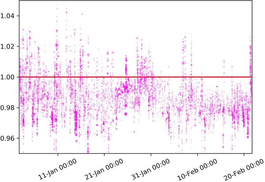
Since releasing the original form of this paper in June 2019, massive liquidation events
around Black Thursday in March 2020 provide additional evidence of deleveraging effects in
the Dai market. Figure 3a depicts a ∼ 50% ETH price cash on 12 Mar. 2020, which precipitated
a cascade of cryptocurrency liquidations. Figure 3b depicts the price effects of these liquidations
15(a) (b)
Figure 3: Black Thursday in March 2020. (a) ∼ 50% ETH price crash (image from On-
ChainFX). (b) liquidation price effect on Dai DEX trades (image from dai.stablecoin.science).
on Dai prices on DEXs. Speculators deleveraging during this event had to pay premiums of
∼ 10% and face consistent premiums > 2% weeks into the aftermath. See [12] for further
discussion of this event.
4 Stability results
We now characterize stable price dynamics of DStablecoins when the leverage constraint is
non-binding. For this section, we make the following simplifications to focus on speculator
behavior:
• The market has fixed dollar demand at each t: wtD At = D. This is consistent with the
stablecoin holder having unit-elastic demand, or having an exogenous constraint to put a
fixed amount of wealth in the stable asset.
• Speculator’s expected Ether return is constant rt = r̂ > 1. This means they always want
to fully participate in the market and is consistent with γ = 0.
D
This is like setting x = D and y = −L. Now the DStablecoin market clearing price is pD
t = Lt .
The leverage constraint (assuming L + ∆ > 0) becomes
−β∆2 + ∆(λ̃(z + D) − 2βL) + L(λ̃z − 2β − βL) ≥ 0.
D
The speculator’s maximization objective becomes r̂∆ L+∆ − ∆, which gives
√
∆∗ = −L + LDr̂.
While we prove a stability result in this simplified setting, we believe the results can be
extended beyond the assumption of constant unit-elastic demand.
4.1 Stability if leverage constraint is non-binding
Prop. 5. Assume wtD At = D (DStablecoin dollar demand) and rt = r̂ (speculator’s expected
Ether return) remain constant. If the leverage constraint is inactive at time t, then the DStable-
coin return is r
pD
t L
= .
pD
t−1 Dr̂
[Link to Proof]
16Supposing that D ≈ L (i.e., the previous price was close to the $1 target) and the constraint
is inactive, Prop. 5 tells us that the DStablecoin behaves stably like the payment of a coupon
on a bond.
Consider estimators for DStablecoin log returns µ̄t and volatility σ̄t computed in a similar
way to Ether expectations in Eq. 2.2.1. When the leverage constraint is non-binding, DStable-
pD
coin log returns remain µ̄t ≈ 0, the contribution to volatility at time t is ln pDt − µ̄t ≈ 0, and
t−1
the DStablecoin tends toward a steady state with stable price and zero variability. The next
theorem formalizes this result to describe stable dynamics of price and the volatility estimator
under the condition that the system doesn’t breach the speculator’s leverage threshold.
Theorem 1. Assume wtD At = D (DStablecoin demand) and rt = r̂ (speculator’s expected
Ether return) remain constant. Let L0 = D and µ̄0 , σ̄0 be given. If the leverage constraint
remains inactive through time t, then
2t −1
(1 − δ)t µ̄0 − δ (1−δ)t −2−t ln r̂, if δ 6= 1/2
2(1−δ)−1
Lt = Dr̂ 2 t
, µ̄t =
2−t µ̄0 − 1 t ln r̂ , if δ = 1/2
2
2
(1−δ)k −2−k+1 (1−δ)
t t−k k
+ (1 − δ)t σ̄02 ,
P
(1 − δ) δ (1 − δ) µ̄ − ln r̂ if δ 6= 1/2
k=1 0 2(1−δ)−1
σ̄t2 = 2
2−t tk=1 2−k−1 (k/2 − 1) ln r̂ − µ̄0 + 2−t σ̄02 ,
P
if δ = 1/2
Further, assuming the constraint continues to be inactive and that δ ≤ 12 , the system converges
exponentially to the steady state Lt → Dr̂, µ̄t → 0, σ̄t2 → 0.
[Link to Proof]
Notice that if the leverage constraint in the system is reached, we can still treat the system
as a reset of µ̄0 and σ̄0 when we reach a point at which the constraint is no longer binding.
While the system subsequently remains without a binding constraint, we again converge to a
steady state starting from the new initial conditions.
Interest rates and trading below $1 A consequence of Theorem 1 is that the DStablecoin
will trade below target during times in which Ether expectations are high. This is empirically
seen in Figure 2b. An interest rate charged to speculators can balance the market (the ‘stability
fee’ in Dai). This can temper expectations by effectively reducing r in Theorem 1. In the stable
steady state, setting the interest rate to offset the average expected ETH return will achieve
the price target. However, this is practically difficult as r changes over time and is difficult to
measure accurately. It also depends on holding periods of speculators. It is an open question
how to target these fees in a way that maintains long-term stability.
4.2 Instability if leverage constraint is binding
When the speculator’s leverage constraint is binding, DStablecoin price behavior can be more
extreme. We argue informally that this can lead to high volatility in our model. The proba-
bility distribution for the leverage constraint to be binding in the next step has a kink at the
boundary of the leverage constraint. In particular, it becomes increasingly likely that the lever-
age constraint is binding in a subsequent step due to deleveraging effects described previously.
Note that feedback of large liquidations on Ether price, if added to the model, will add to this
effect.
17DStablecoin Returns by Constraint Activity
103 Active DStablecoin Volatility vs. Memory Parameter
Inactive 0.05 Ether volatility
102 70 percentile
0.04 95 percentile
Volatility (Daily)
Density 101
100 0.03
10−1 0.02
10−2 0.01
−0.10 −0.05 0.00 0.05 0.10 0.15 0.20
Log return 0.00
0.1 0.2 0.3
Memory Parameter
(a) Histogram of DStablecoin returns
when leverage constraint is binding vs. (b) Heat map of volatility under different
non-binding with constant r̂. speculator γ = δ memory parameters.
Figure 4: DStablecoin volatility, 10k simulation paths of length 1000.
We show such instability computationally in Figure 4a in simulation results. In this figure,
the shape of the inactive histogram reflects the speculator’s willingness to sell at a slight discount
when the leverage constraint is non-binding due to the constant r̂ assumption.
We relax this assumption in Figure 4b, which shows the effects on volatility of different
speculator memory parameters. This figure is a heat map/2D histogram. A histogram over
y-values is depicted in the third dimension (color: light=high density, dark=low density) for
each x-value. Each histogram depicts realized volatilities across 10k simulation paths using the
simulation setup introduced in the next section and the given memory parameter (x-value).
Horizontal lines depict selected percentiles in these histograms. The dotted line depicts the
historical level of Ether volatility for comparison.
In Figure 4b, volatility is bounded away from 0 even in non-binding leverage constraint
scenarios; the distance increases with the memory parameter. This happens because r updates
faster with a higher memory parameter. As the speculator’s objective then changes at each step,
the steady state itself changes. Thus we expect some nonzero volatility, although it remains
low in most cases.
In not-so-rare cases, however, volatility can be on the order of magnitude of actual Ether
volatility in these simulations. As seen in Figure 5, this result is robust to a wide range of
choices for the speculator’s risk constraint. This suggests that DStablecoins perform well in
median cases, but are subject to heavy tailed volatility.
5 Simulation Results
We now explore simulation results from the model considering a wide range of choices for the
speculator’s risk constraint. Unless otherwise noted, the simulations use the following parameter
set with a simplified constant demand assumption (D = 100) and a t-distribution with df=3 to
simulate Ether log returns. Cryptocurrency returns are well known for having very heavy tails.
This choice gives us these heavy tails with finite variance. Note, however, that this doesn’t
capture path dependence of Ether returns. We instead assume Ether returns in each period
are independent. We run simulations on 10k paths of 1000 steps (days) each. This is enough
time to look at short-term failures and dynamics over time. The simulation code is available
at https://github.com/aklamun/Stablecoin_Deleveraging.
18Parameter Value Rationale
n0 400 4x initial collateralization > typical Dai level
r0 1.00583 Historical daily Ether mult. return 2017-2018
µ0 0.00162 Historical daily Ether log return 2017-2018
σ0 0.027925 Historical daily Ether volatility 2017-2018
γ=δ 0.1 ∼ Recommended value [15]
β 1.5 Threshold used in MakerDAO’s Dai
α ∼ 1.28 Value assuming normal distr. + a = 0.1
b 1 Consistent with VaR constraint
Note that our simulations study daily movements. We choose this time step to examine
these systems under reasonable computational requirements. More realistic simulations might
study intraday movements. One plausible scenario of a Dai freeze is if the price feed moves too
far too fast instraday, so that speculators don’t have enough time to react before liquidations
are triggered and keepers (who perform actual liquidations) are unable to handle the avalanche
of liquidations. As the price feed in Dai faces an hourly delay in the price feed, hourly time
steps are a natural choice for follow-up simulations. This said, daily time steps can actually
be reasonable due to a behavioral trend in Dai data: most Dai speculators realistically don’t
track their positions with very high frequency as supported by overall high liquidation rates.
5.1 Speculator behavior affects volatility
We compare DStablecoin performance under the following speculator behaviors encoded in the
risk constraint.
Name Speculator risk constraint
VaRN.1 VaR using a = 0.1 + normality assumption
VaRN.01 VaR using a = 0.01 + normality assumption
VaRM.1 VaR using a = 0.1 + heavy-tailed assumption
VaRM.01 VaR using a = 0.01 + heavy-tailed assumption
AC1 Anti-cyclic constraint, b = −0.5, α = 0.01
AC2 Anti-cyclic constraint, b = −0.5, α = 0.02
RN Risk neutral, only faces liquidation constraint
Figure 5 compares the effects on volatility of these behavioral constraints under various Ether
return distributions. These figures are heatmaps/2D histograms similar to that in Figure 4b.
The results suggest that DStablecoins face significant tail volatility (on the order of Ether
volatility) even under comparatively ‘nice’ assumptions on Ether return distributions, such
as with significant upward drift (Figure 5b) and a normal distribution (Figure 5c). Figure 7
depicts relative (% difference) mean-squared difference of simulated volatility for the different
risk management methods vs. a risk neutral speculator. The mean-squared difference is large,
suggesting that the speculator’s risk management method has a large effect on volatility.
The results suggest how speculator behavior can affect DStablecoin volatility within the
model. Stricter cyclic risk management (e.g., VaR) on the part of the (single) speculator can
lead to increased DStablecoin volatility without improving the safety of the system. Whether
countercyclic (setting constraint to increase leverage during downturns) or cyclic (setting con-
straint to decrease leverage during downturns), the resulting DStablecoin volatility is connected
with how narrow the feasible region for the constraint becomes. A risk neutral speculator,
which has the widest feasible region for the constraint, leads to the lowest volatility. Stricter
risk management serves to reduce the feasible region. Note that these results may be different
19You can also read