HERMES: Mobile System for Instability Analysis and Balance Assessment
←
→
Page content transcription
If your browser does not render page correctly, please read the page content below
HERMES: Mobile System for Instability Analysis and Balance
Assessment
HYDUKE NOSHADI and FOAD DABIRI, University of California at Los Angeles and Google Inc.
SHAUN AHMADIAN, NAVID AMINI, and MAJID SARRAFZADEH, University of California at
Los Angeles

We introduce Hermes, a lightweight smart shoe and its supporting infrastructure aimed at extending gait
and instability analysis and human instability/balance monitoring outside of a laboratory environment.
We aimed to create a scientific tool capable of high-level measures, by combining embedded sensing, signal
processing and modeling techniques. Hermes monitors walking behavior and uses an instability assessment
model to generate quantitative value with episodes of activity identified by physician, researchers or
investigators as important. The underlying instability assessment model incorporates variability and
correlation of features extracted during ambulation that have been identified by geriatric motion study
experts as precursor to instability, balance abnormality and possible fall risk. Hermes provides a mobile,
affordable and long-term instability analysis and detection system that is customizable to individual users,
and is context-aware, with the capability of being guided by experts. Our experiments demonstrate the
feasibility of our model and the complimentary role our system can play by providing long-term monitoring
of patients outside a hospital or clinical setting at a reduced cost, with greater user convenience, compliance
and inference capabilities that meet the physician’s or investigator’s needs.

Categories and Subject Descriptors: C.3 [Computer Sysytems Organization]: Special-Purpose and Ap-
plication Based System—Real-time and embedded systems; J.3 [Compute Applications]: Life and Medical
Sciences—Medical information system; H.1.2 [Information Systems]: User/Machine Systems—Human
information processing
General Terms: Design, Experimentation, Human Factors, Measurement
Additional Key Words and Phrases: Instability modeling and analysis, Plantar Pressure Sensing, Sensor
Selection, Wireless Health, Balance and Instability assessment
ACM Reference Format:                                                                                                   57
Noshadi, H., Dabiri, F., Ahmadian, S., Amini, N., and Sarrafzadeh, M. 2013. HERMES: Mobile system for
instability analysis and balance assessment. ACM Trans. Embedd. Comput. Syst. 12, 1s, Article 57 (March
2013), 24 pages.
DOI: http://dx.doi.org/10.1145/2435227.2435253

1. INTRODUCTION
Embedded networked systems and wide area cellular wireless systems are becoming
ubiquitous in applications ranging from environmental monitoring to urban sensing.
These technologies have recently been adopted to support the emerging work in Wire-
less Health. Wireless Health merges data, knowledge, and wireless communication
technologies to provide health care and medical services, such as prevention, inter-
vention, diagnosis, and rehabilitation outside of the traditional medical enterprise.

Author’s addresses: H. Noshadi, Computer Science Department, University of California at Los Angeles;
email: hyduke@cs.ucla.edu.
Permission to make digital or hard copies of part or all of this work for personal or classroom use is granted
without fee provided that copies are not made or distributed for profit or commercial advantage and that
copies show this notice on the first page or initial screen of a display along with the full citation. Copyrights for
components of this work owned by others than ACM must be honored. Abstracting with credit is permitted.
To copy otherwise, to republish, to post on servers, to redistribute to lists, or to use any component of this
work in other works requires prior specific permission and/or a fee. Permissions may be requested from
Publications Dept., ACM, Inc., 2 Penn Plaza, Suite 701, New York, NY 10121-0701 USA, fax +1 (212)
869-0481, or permissions@acm.org.
c 2013 ACM 1539-9087/2013/03-ART57 $15.00
DOI: http://dx.doi.org/10.1145/2435227.2435253

          ACM Transactions on Embedded Computing Systems, Vol. 12, No. 1s, Article 57, Publication date: March 2013.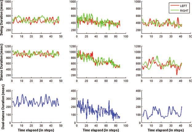
57:2                                                                                          H. Noshadi et al.

Ever-increasing opportunities in health care have thus motivated researchers in Com-
puter Science and Electrical Engineering to develop technologies that can be adopted
in the medical and physiological fields to serve the recently growing demand of low cost
and widely accessible health care services.
   Fall related injuries are one of the challenges that our health care system is facing to-
day. In 2002, more than $19 billion was spent on all fall injuries for people 65 and older
alone [Stevens et al. 2006]. This number may exceed $55 billion in 2020 (adjusted for in-
flation) [Englander et al. 1996] [CDC 2008]. Even more surprisingly, direct and indirect
costs associated with falls are $75 to $100 billion in the U.S. annually [Comodore 1995].
   Mean hospitalization cost of falls was $17,500 in 2004 [Roudsari et al. 2005]. A recent
study shows that hospital and long-term-care costs resulting from falls in nursing
homes and long term care facilities has been estimated to be an average of $6, 200 per
year per resident [Carroll et al. 2008].
   Even with this knowledge, the current health care system does not have the capabil-
ity of monitoring an individual’s fall risk outside a hospital setting. Although regular
doctor visits are helpful, it can be too expensive and inconvenient for most patients to
perform at a granularity that is effective; that is why a low-cost and more proactive sys-
tem is needed. In hopes of mitigating the economic and emotional costs of falls, we have
developed Hermes, a lightweight, non-invasive system for everyday use to aid ordinary
individuals in assessing their fall risk. Although Hermes alone does not directly prevent
falls, it does allow primary-care providers to make assessments that allow preventa-
tive measures to be taken. The cost associated with the current version of the Hermes
prototype is approximately $400 and will decrease under commercial production.
   The remainder of this article is organized as follows. In Section 2 we discuss related
work and introduce the article’s main contributions. In Sections 3 and 4 we describe
hardware and software architecture that comprise Hermes. In Section 5 our proposed
instability assessment model and framework is introduced. Section 6 demonstrates
our investigation on sensor selection and placement to minimize hardware and energy
costs. Section 7 describes the signal processing stack used to extract temporal and
spatiotemporal parameters in order to assess consistency in human walk. Finally, we
conclude the article with Sections 8 and 9 by illustrating the feasibility of our model
and discussing future work.
2. RELATED WORK
To better understand the potential impacts of Hermes we present several methods cur-
rently used by physicians and geriatric experts for assessing instability and measuring
imbalance. In general these methods can be categorized into two major classes. The first
set of methods are clinical tests that rely mainly on the trained eyes of a physician for
evaluation and diagnosis. One benefit of this class of tests is that little or no equipment
is required. The second major class of tests are those that occur in motion laboratories
using expensive motion capture equipment along with pressure-based devices; conse-
quently these methods render highly quantitative and accurate results. With recent
advances in embedded and wireless communication, a third class has emerged from
academic and industry-based research labs based on wearable and mobile platforms
for instability and gait analysis. Having introduced the main methods we now explore
them in detail.
   Clinical methods. Methods such as clinical balance tests are benchmarks to measure
static, reactive and anticipatory postural control for comparison against standardized
scores. The Berg Balance Test is one such test that measures balance based on the
performance of a predefinded set of tasks [Thorbahn and Newton 1996]. It consists
of 14 mobility tasks of varying degrees of difficulty from easy to difficult. Clinicians
score each task on a scale from 0 to 4, where 0 means that the subject is not able to

        ACM Transactions on Embedded Computing Systems, Vol. 12, No. 1s, Article 57, Publication date: March 2013.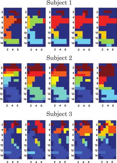
HERMES: Mobile System for Instability Analysis and Balance Assessment                                        57:3

complete the task and 4 if the subject was able to complete the task. A total score
is tailed out of 56. A pre-set score has been established in the literature to identify
subjects at increased risk for falls. [Yenets et al. 2007]. Another test, the Up-and-Go
Test, compares the time that it takes a patient to stand up from a sitting position, walk
3 meters, turn around and return to sitting position [Podsiadlo and Richardson 1991].
The measured time is compared against standardized ranges to assess the patient’s
fall risk level. Unlike the previous two tests, the Functional Reach Test is a stationary
test that measures the maximum forward reach of an individual on a fixed base of
support [Behrman et al. 2002]. It has been demonstrated that this test can detect
balance abnormality and its change over time. Despite its convenience and low-cost
administration, clinical balance tests have severe limitations. For one, they do not
produce the kinetic and kinematic data necessary to determine the gait parameters
of the patient, which are important for diagnosing problems. The duration and the
controlled setting of these experiments require a great deal of extrapolation to the
diverse environmental settings typical of daily activities.
  Gait Labs. Through state-of-the-art pressure and motion capture systems, gait mea-
surement labs address the intrinsic parameters that clinical balance tests fail to mea-
sure. One such system called a force plate [Bertec 2008] measures ground reaction
forces during stance and ambulation. Using these measures posturography [Mon-
sell et al. 1997] can quantify postural control in static and dynamic condition and
determine postural sway. Since force plates are small in diameter most of the measure-
ments are derived from recordings of a single step. Instrumented walkways such as
GaitRite [GaitRite 2008] try to extend the duration of experiments to multiple steps
by using pressure sensitive floor mats ranging from 3-5 meters in length. This allows
for greater visibility into spatiotemporal gait parameters as investigated in [Cutlip
2000]. Camera-based motion capture systems such as Vicon [Vicon 2008] provide the
most extensive view of kinematic parameters of human gait but such systems are ex-
tremely expensive and fairly rare. Less expensive motion capture systems have been
proposed for motion analysis but mostly with the ultimate goal of human tracking and
not biomechanical assessment [Davis and Gao 2003; Niyogi and Adelson 1994; Yam
et al. 2004; Johnson et al. 2003; Gatech 2002].
  Mobile. To address the lack of mobility in these systems Pedar utilizes in-sole pres-
sure sensing hardware and a PDA sized data-acquisition board to collect pressure
distribution for each foot. The collected data is passed through signal processing soft-
ware to derive temporal gait parameters as well as center-of-pressure displacement
[Novel 2008b]. Similar to the aforementioned systems, although accurate, Pedar is ex-
pensive (over $20,000 for the basic measuring system [Novel 2008a]) and cannot easily
be deployed in a non-laboratory setting.
  Low-cost, pressure-based systems like Hermes have been proposed for various health
applications including foot ulcer prevention, fitness, and extraction of basic gait param-
eters. One such system [Morley et al. 2001; Maluf et al. 2001] quantifies the condition
to predict the progression of ulceration in diabetic patients suffering from neuropathy.
A wireless enabled “smart shoe” has been introduced in Dabiri et al. [2008], which
identifies abnormal pressure under the foot and pre-emptively alerts patients and care
givers. Pressure sensing based system has been introduced by Zhu et al. [1990], which
measures pressure distribution under the feet by utilizing force sensitive resistors and
quantifies the difference between different gait events such as walking and shuffling
and mentions the need to have the test over the large population to collect data in log
period of time [Zhu et al. 1991, 1993]. Possibility of falling and existence of pattern
in gait has been studied, which is using temporal parameters of the gait extracted
by two pressure sensor (one on the toe and the other on the heel) [Hausdorff et al.

ACM Transactions on Embedded Computing Systems, Vol. 12, No. 1s, Article 57, Publication date: March 2013.
57:4                                                                                           H. Noshadi et al.

Fig. 1. Hermes takes advantage of data modeling to shift the accuracy and inference capability of the mobile
platform.

1995, 1999, 2001, 1996]. The most relevant application to our work is the shoe inte-
grated wireless sensor system introduced in Bamberg et al. [2008]. This system uses
a combination of pressure sensors, a 3-axis accelerometer and a gyroscope to extract
spatial and spatiotemporal gait parameters. The system is designed to be worn in any
shoe while having little impact on gait parameters. The shoe is capable of long-term
data collection as well as accurate detection of events such as heel strikes and toe
lifts, in addition to the foot orientation and position, all of which are important for gait
analysis.
   The aforementioned clinical techniques and commercial systems lack quantitative
and reproducible measures (such as those acquired through an electronic device) or
are limited to controlled environment (such as lab) and only support short duration
examinations. Even recent low-cost, mobile alternatives lack data modeling techniques
to properly assess instability and its progression.
   Our system is motivated by Maki [1997] and recent findings in Hausdorff [2007] that
show gait variablilty to be an effective measure to analyze the risk of falling. However,
the discussion of which gait parameters and how they vary is still an active discussion
in the medical literature. Although these new findings have been critical to our un-
derstanding of instability and fall risk, they require large data sets that span a long
interval of time; since only then are variability measurements meaningful. Low-power,
wireless mobile platforms can address this issue, but they are prone to low data fidelity.
To address this issue by taking instability analysis, cost and power into consideration,
we developed Hermes, which draws upon data modeling techniques (Figure 1). Hermes
is designed to provide a gait and instability analysis model configurable by researchers
and health care professionals to meet their needs. To make this possible, our research
contributions are threefold:

(1) A mobile sensing platform integrated in the shoe that is non-invasive, customiz-
    able, low-power, and low-cost and a processing stack responsible for synchronizing
    multiple sensing channels, handling malformed signals, extraction of temporal and
    spatiotemporal features and their associated timeseries parameters.
(2) Development of an instability assessment model that incorporates temporal,
    spatiotemporal factors to assess balance and instability; and a corresponding set
    of experiments to show its feasibility.
(3) Empirical study of Pedar [Novel 2008b] to model its behavior to be able to
    design such a system that can operate in low-power environment with low-cost
    components.

         ACM Transactions on Embedded Computing Systems, Vol. 12, No. 1s, Article 57, Publication date: March 2013.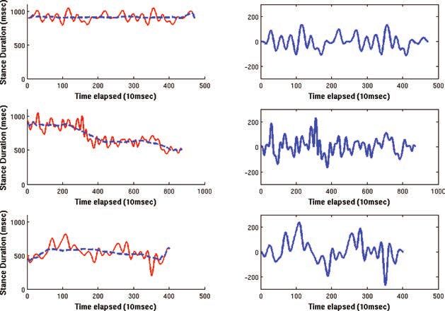
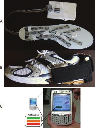
HERMES: Mobile System for Instability Analysis and Balance Assessment                                        57:5

Fig. 2. Hardware (a) A single shoe insole unit, this is the entirety of the required hardware, which can
be used in different types of shoes of the same size. (b) This is a shoe with the insole unit placed inside,
with the microcontroller strapped to the outside. (c) After wireless data transfer to a mobile device, fall risk
assessment occurs here.

3. HARDWARE ARCHITECTURE
The Hermes hardware architecture consists of the components shown in Figure 2 : off
the shelf, low-cost sensors, integrated into the insole and shoe, measuring pressure,
motion and rotation; embedded computing platform to support data acquisition, syn-
chronization, low-power Bluetooth and radio interfaces; a personalized device, which
provides intermediate storage and is Bluetooth-enabled and has a Wi-Fi and GPS in-
terface. The personal device is capable of processing the sensor readings received from
the shoe in real-time, as well as sending the received data or a subset of the data to a
centralized server through Wi-Fi or GPRS. In addition, the personalized device is ca-
pable of providing feedback to the user both visually and non visually, such as through
vibration and sound notification.
   The data is transferred to the centralized server and can be used for future in-depth
analysis and verification purposes. The collected data in the centralized server can be
aggregated with the data associated with the user’s location and environment to per-
form more elaborate analysis of the collected data. The collected data can be uploaded
to a server opportunistically, to increase battery life, and it can decide when to upload
based on some kind of schedule determined by the specific situation. For example if
Wi-Fi access is rare, it may just upload whenever it comes into range, or if Wi-Fi access
is abundant, it may upload on a daily schedule. Once the data has been uploaded, it
becomes unnecessary and undesirable to keep it stored on the device. Although, with a
standard 1GB microSD card, we can store nearly 100 hours worth of continuous data.
The specific device we used in our tests has an operational battery life in the range of
7.5 hours (talk time) up to 250 hours (idle time) [HP 2008]. This gives us a very rea-
sonable flexibility with the amount of time a user can use our system away from a lab.

ACM Transactions on Embedded Computing Systems, Vol. 12, No. 1s, Article 57, Publication date: March 2013.
57:6                                                                                               H. Noshadi et al.

            Sensor Reading (raw)
                                   300
                                                                                                 Pedar
                                   200                                                           Hermes

                                   100

                                     0
                                      0   50   100   150         200           250   300   350        400
                                                           Time elapsed (ms)

Fig. 3. Readings of sensors from Pedar and Hermes in the same location. The readings are inherently noisier
for Hermes due to the lack of conditioning circuits in the current prototype. The reason to have nonzero value
is that the foot can still apply some pressure on the insole, due to tightness of the shoe, while the foot is on
the air.

  To collect and relay the data, we have used MicroLEAP [Au et al. 2007] sensing
platform, which has been designed at UCLA. MicroLEAP has an MSP430 embedded
processor and it uses Bluetooth communication stack.

3.1. Embedded Sensors
Hermes is equipped with a set of non-invasive sensors. This set of sensors on the shoe
consists of pressure sensors, a 3-axis accelerometer and 3 single axis gyro, where the 3-
axis accelerometer and a 2-axis gyro is embedded on the MicroLEAP and a single-axis
gyro is connected externally.
  Pressure Sensors are ultra-thin and piezoresistive sensors that can easily be spread
across the insole [Tekscan 2008]. The FlexiForce force sensor is an ultra-thin (thick-
ness of 0.127 mm) and flexible printed circuit consisting of two layers of substrate
(polyester/polyimide) film. On each layer, a conductive material is applied, followed
by a layer of pressure-sensitive ink. The electrical resistance of FlexiForce sensors is
inversely proportional to the force applied to the active sensing area, which has a diam-
eter of 9.53 mm. The sensor range of 0–100 lbs can be used for patients with different
weights. A simple voltage divider circuit has been used to produce an output voltage
corresponding to resistance values. Each FlexiForce sensor was individually calibrated
using an accurate digital weight scale and the accuracy of calibration results was
comparable to those provided by the manufacturer.1
  3-D Accelerometer used in this system is a low-power accelerometer by Analog
Devices [Analog 2010a] with the capacity to measure acceleration in the range of ±3g.
Before conducting each experiment, we calibrated the accelerometer by aligning its
axes parallel and perpendicular to gravity (corresponding to nominal output of 1 and
0 g, respectively) and adjusted the gain and offset accordingly.
  Gyroscopes used on Hermes are 3 single axis gyros, with measurement range of 150 ◦
/s [Analog 2010b], two of which are embedded inside the MicroLEAP platform and the
3rd one is connected externally. The accelerometer and gyro are used to detect the linear
acceleration and angular movement of each foot. With regards to gyroscopes, through-
out all experiments, we have relied on specifications given by the manufacturers.
  The MicroLEAP is mounted in the back of the shoe, such that one axis of accelerom-
eter and gyro are aligned with body. The force sensors embedded inside each insole
measure the forces applied to the bottom of each foot and are connected to the process-
ing unit through a 16 bit ADC channel. (See Figure 3).

1 We use conductance as opposed to resistance in the calculations, since the force measured with these sensors
have a linear relation with the conductance, otherwise it is evident that both represent the same physical
properties of the sensor.

          ACM Transactions on Embedded Computing Systems, Vol. 12, No. 1s, Article 57, Publication date: March 2013.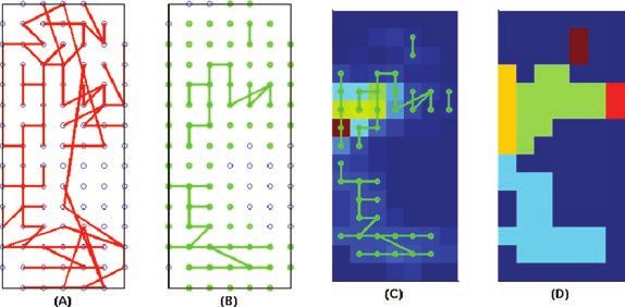
HERMES: Mobile System for Instability Analysis and Balance Assessment                                        57:7

Fig. 4. Diagram of software architecture of Hermes, consists of the embedded software (running on the
shoe) and the personalized device software.

4. SOFTWARE ARCHITECTURE
The software architecture in our system consists of two main components as shown in
Figure 4, which are: the embedded software running on each processing unit embedded
inside the shoe and software running on personalized device.
   The embedded software running on each processing unit is responsible for data
acquisition, preliminary data and signal analysis, time synchronization between the
two shoes, and data transfer to the personalized device or pervasive environment. The
sensor values are collected based on appropriate time interval and after performing
a filtering on small samples window the collected signal is transferred over radio
interface or Bluetooth. Sensor data collected from data acquisition units in the shoe
can be streamed to a variety of devices, as long as they are Bluetooth enabled. For
experimental purposes we interface the shoe with both a PDA and a PC.
   The Software system on the personalized device is responsible for computational
and storage intensive tasks such as, visual data display, notification and guidance.
It has the following three layers of architecture: network interface, processing, and
presentation.
4.1. Network Interface Layer
In the network layer, streamed data packets received from the shoe are buffered,
ordered, and batched before sending to the processing layer.
4.2. Processing Layer
The processing layer is responsible for logging streamed data, signal processing, and
providing an API to each of its components. The processing unit performs different
signal processing techniques such as filtering, feature selection and classification to
convert a raw signal into a meaningful chain of data, which can then be interpreted by
a model, in this case by the instability assessment model. The logging module stores
received data from each sensor through the network layer. The logged data can be used
for a variety of purposes, such as displaying the activity on the UI and monitoring
patterns over a long period of time.

ACM Transactions on Embedded Computing Systems, Vol. 12, No. 1s, Article 57, Publication date: March 2013.
57:8 H. Noshadi et al.
4.3. Presentation Layer
Users can interact with the processing and network layers through the provided API.
The presentation layer displays the data read from each pressure sensor and accelerom-
eter in real time. It also has the capability of playing the logged data for a desired period
of time. Through the presentation module (i.e., graphical user interface), real time nor-
malized data streams from each pressure sensor and accelerometer and is displayed in
separate plots for each sensor type. Finally, the notification unit is triggered by events
that occur in the processing unit, which can be an indication of an emergency, an ab-
normal situation, or any event that requires attention. The notification component is
responsible for propagating the detected abnormality to the user via the user interface
and/or various other mediums, such as SMS, email, and phone calls.
5. INSTABILITY ANALYSIS
Instability is defined as a an individual’s inability to control and maintain proper bal-
ance and orientation [Yenets et al. 2007]. The presence of instability has been identified
as a primary cause of falls. Common fall risk factors include hearing, vision, motor, and
cognitive impairments resulting from aging as well as chronic conditions such as di-
abetes [ASTHO 2006; Sorock 1988]. These conditions affect the normal ambulatory
pattern, which in turn alter gait parameters, such as step length, double limb support,
cadence, time for each taken step, gait speed, stride length, and stance-to-swing phase
ratio [Yenets et al. 2007].
We define the spatial and temporal parameters according to Whittle [2007] as follows.
(1) Step length is the distance from a point of contact with the ground of one foot to
the following occurrence of the same point of contact with the other foot. This can
generally be thought of as the distance one foot moves forward in front of the other.
(2) Step time is the time taken for each step.
(3) Cadence is the number of steps taken per second.
(4) Stride length is defined as the distance between successive points of initial contact
of the same foot. It consists of two steps lengths, left and right.
(5) Gait speed is the product of stride length and cadence.
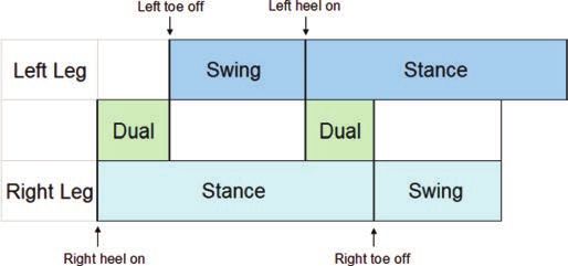
(6) Stance-to-swing ratio, where the stance phase is the time from heel-contact to toe-
off, and the swing phase is the time between toe-off and heel-contact. An ambulation
contains 60 percent of stance phase and 40 percent of swing phase (Figure 5).
(7) Dual stance (Double limb support) is the time that both feet are in contact with the
ground.
(8) Pressure correlation is the correlation of the pressures recorded in each step with
the previous steps.
Destabilizing forces imposed by the environment or degradation in visual, vestibu-
lar, motor and somatosensory systems would manifest themselves in gait changes and
hence gait parameters. Furthermore, variability in these parameters as indicated by
[Maki 1997] is an important factor in fall prediction. Having talked with experts at the
UCLA VA Hospital, we introduced an instability assessment model that addresses most
of the factors associated with physiological, cognitive, visual, motor and also environ-
mental factors to assess instability. We perform instability assessment by aggregating
the parameters extracted in each step, as shown in Figure 6.
In the pre-processing step, the time series signal is filtered and segmented based on
the implemented segmentation rule. The segmentation rule categorizes each segment
into classes defined by the segmentation policy. The policy is set by physician or the in-
terested party in the instability assessment result. The segmentation rule identifies the
granularity of analysis. Some examples of segmentation rules are: fixed time interval,
ACM Transactions on Embedded Computing Systems, Vol. 12, No. 1s, Article 57, Publication date: March 2013.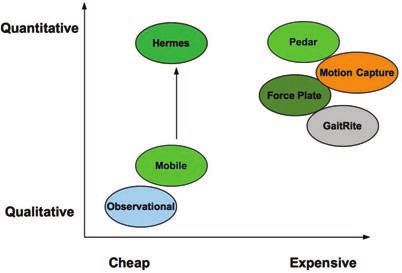
HERMES: Mobile System for Instability Analysis and Balance Assessment                                        57:9

Fig. 5. Gait cycle beginning with the right heel making initial contact with the ground, where walking
direction is left to right. Figure illustrates stance/swing phases for both legs, as well as the double limb
support.

Fig. 6. Processing stack shows the steps implemented for assessing instability and risk computation. Fil-
tering and segmentation is part of pre-processing. In the processing stage, temporal, spatiotemporal and
consistency features are extracted and finally in the Risk assessment step the risk associated with each
segment is computed.

activity based (e.g., walking or running) or based on a set of events triggered by exter-
nal factors (e.g., based on geographical location using an external signal received from
GPS on personalized device). In the processing step, first the gait cycles are identified
on each segment. Then the interest points are detected in each cycle, which are used for
feature extraction. Meanwhile the correlation of neighbor steps in the same segment of
the each signal, received from pressure based and non pressure based sensors is com-
puted. The goal is to quantify the similarity, harmony, and step consistency. For each
step a correlation relation is generated that is relative to the previous close steps and
the baseline steps of the same signal to measure variation. Then the gradual shift of
each extracted feature is computed over time. The gradual shift represents the change
in walking pace and is used as the baseline to measure the variability of detected tem-
poral and spatiotemporal features. Once the trends for the features are computed the

ACM Transactions on Embedded Computing Systems, Vol. 12, No. 1s, Article 57, Publication date: March 2013.
57:10                                                                                         H. Noshadi et al.

variability of each feature is calculated relative to the trend. Finally, in the instability
assessment section, for each segment we compute the instability based on Equation (1),
where VT and VST are the variance of temporal and spatiotemporal parameters in the
segment. VT and VST are computed based on Equation (1), where τi is the variance
of temporal feature i and σ j is the variance of spatiotemporal feature j. αi and γ j
are the coefficients that indicate the importance of a particular feature and they are
constrained by Equation (2). The coefficients can be set by physicians, clinicians and
domain exports to tailor the instability assessment to best fit the individual patient.


                                                      n
                                                                       m
                           Risk = VT + VST =                αi Vτi +         γ j Vσ j                         (1)
                                                      i=1              j=1


                                                        n
                                                                     m
                                                              αi +         γ j = 1.                           (2)
                                                        i=1          j=1

  Our instability assessment engine aggregates the computed risk for each class of
segments, defined by a segmentation policy, and produces a matrix, which maps each
class to a set of risk values. The presence of risk values is used to generate the statistics
regarding the instability in each class, which will be used by physicians for diagnosis
and monitoring purposes (see Figure 6).

6. SENSOR CLUSTERING
Hermes utilizes a limited set of pressure sensors for the purpose of realtime monitoring
of the human locomotion and pressure distribution. A very important question to be
answered is the number and location of these pressure sensors. Mobility and wear-
ability requirement of the system imposes some limitations in terms of the number
of pressure sensors that can be incorporated. Furthermore, due to physical nature of
human physiology and motion patterns, it is only natural to assume that there are
certain locations beneath the foot that the pressure data is either very similar and/or
mutually dependent. In this section, we study the correlation and dependance across
different pressure points and introduce a sensor clustering methodology that is used to
identify locations and sensors that capture most of the dynamics of human locomotion.
   To get a better understanding of the signals resulting from the exertion of pressure by
the feet we turned to Pedar [Novel 2008b]. Pedar is an accurate and reliable pressure
distribution measuring system for monitoring local loads between the foot and the
shoe. It is comprised of insoles equipped with a grid of pressure sensors and a data
acquisition unit capable of local storage and transmission to a PC over wireless or
wired connection.
   The console of the Pedar system is covered with 99 pressure sensors to cover almost
the whole bottom of the foot. In this section, we aim to optimize the system performance
through ÓSensor SelectionÓ. Sensor selection, intuitively, refers to selecting a subset
of the available sensors and only monitor the data from this set. The reason to pursue
such an objective lies in the fact that sampling each sensor, storing the data from it and
transmitting the data requires resources such as power and memory and unless neces-
sary, there is no justification to allocate these resources in a low power mobile system.
   Pedar enables us to utilize its large number of sensors and extract the most effective
positions in the bottom of the foot and therefore we equip Hermes accordingly. In other
words, Pedar is our view of the whole space of possible sensor locations and our goal
is to find the best and critical locations that is needed for constant monitoring. These
locations are where the Hermes sensors are positioned.

        ACM Transactions on Embedded Computing Systems, Vol. 12, No. 1s, Article 57, Publication date: March 2013.
HERMES: Mobile System for Instability Analysis and Balance Assessment 57:11
6.1. Problem Formulation
Let’s first formulate the sensor selection problem analytically. We model the sensors
on the insole with a graph G(V, E), where V = {s1 , s2 . . . , sn} is the set of nodes in
the graph representing the sensors and E = {(si , s j ) . . .} is the edges amongst them.
We will describe the definition of an edge in Section 6.2. The objective we seek is to
select a minimum subset of sensors that will not affect the precision of the instability
analysis in this article. Since the objective under study (i.e., instability analysis) is a
function of the variance of temporal (VT ) and spatiotemporal (VST ) features, we state
the sensor selection objective with the function , which is the error introduced to these
parameters as a result of sensor selection. The accuracy can formally be represented
as a constraint to an optimization problem in the form of S⊆V (VT + VST ), which
indicates the accuracy in VT + VST when the subset S of the sensors are selected. With
the introduction of this constraint, the sensor selection problem can be defined as:
minimize|S|
where : S ⊆ V
s.t. : S (VT + VST ) ≥ η, (3)
where η is the target accuracy and ideally: η = V (VT + VST ), which means we have all
the sensor to measure the temporal and spatiotemporal features. We will not analyt-
ically solve the problem but will propose a selection methodology that experimentally
leads to an acceptable efficient solution.
6.2. Sensor Selection
We propose an empirical solution to this problem supported by simulation and exper-
imental results. In this study, we make use of two key concepts from data modeling:
Variability to provide information about the shape of the signal and how it is distributed
and Correlation to provide information about how similar the shape (not amplitude) of
the individual sensing channels are to one another. For our study we focused on using
correlation to combine sensor readings that have similar shapes and using variability
to determine which sensors contributed most to the underlying phenomenon. To do so,
we first construct the edges of the graph G:
∀vi , v j ∈ V : ei j ∈ E
and : w(ei j ) = ρ(vi , v j ),
where w(ei j ) is the weight assigned to the edge ei j and is equal to the correlation factor
of the data from sensors vi and v j : ρ(vi , v j ).
Once the edges in G are constructed, the process of sensor selection can be summa-
rized as the following three steps: Removing weak edges, finding strong components
and selecting a sensor from each component.
For the first step we remove all the edges where ρ(vi , v j ) < δ. The threshold δ can
be estimated using the correlation distribution across all the edges and its relation to
edges distance based on the objective of the problem Figure 7 shows the distribution of
pairwise correlation among all the sensor pairs. As the figure suggests due to nature of
human walk both positive and negative correlation values are present. Figure 8 shows
the relationship between distance of two sensors and their correlation among all pairs
with positive correlation values. We chose δ = 0.7 since it would leave us with enough
edges that would connect nodes in different active pressure area under the foot). After
the edge removal we end up with the graph G :
G = (V, E )
where : E ⊂ E, ∀ei j ∈ E , ρ(vi , v j ) ≥ δ.
ACM Transactions on Embedded Computing Systems, Vol. 12, No. 1s, Article 57, Publication date: March 2013.57:12 H. Noshadi et al.
1000
900
800
700
Sensor Pairs
600
500
400
300
200
100
0
−0.5 0 0.5 1
Correlation Value
Fig. 7. Distribution of pairwise linear Pearson’s correlation among all the sensor pairs.
Correlation between each 2 sensors sorted by distance
1
0.9
0.8
0.7
0.6
correlation
0.5
0.4
0.3
0.2
0.1
0
0 1 2 3 4 5 6 7 8
Distance
Fig. 8. Distance vs Pearson’s correlation of each two pairs of sensors that have positive correlation value.
Sensors in Pedar’s insole construct a grid. We define the distance between each two sensor as the shortest
path between them in the grid.
In the next stage we find all the connected components of G and call them Ci (Vi , Ei ).
Each connected component is believed to be a set of sensors that are highly correlated.
For each sensor v in a given component Ci we compute the “strength” of the sensor:
λ(v)
λ(v) = w(evu) + w(euw ), (4)
u∈N(v) u,w∈N(v)
where N(v) is the set of the neighbors of v in the component that v belongs to. Intu-
itively, Equation (4) indicates that a strong sensor is not only strongly connected to its
neighbors (first term in the right hand side of the equation) but also its neighbor in
ACM Transactions on Embedded Computing Systems, Vol. 12, No. 1s, Article 57, Publication date: March 2013.HERMES: Mobile System for Instability Analysis and Balance Assessment 57:13
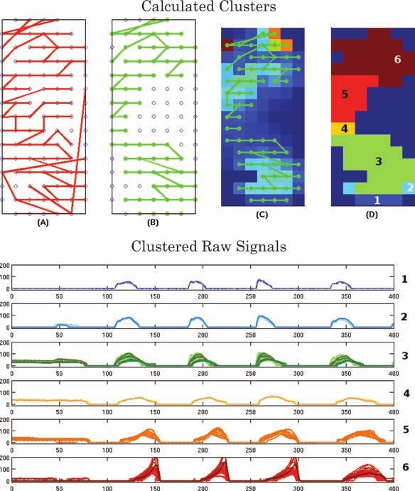
Fig. 9. Sensor clustering involves : Removing weak (a, b). Finding strong components (c). Choosing a sensor
from final cluster set (d).
the component are also highly correlated (second term in the right hand side of the
equation).
For each component Ci , the selected sensor si∗ will become:
si∗ = argmax(λ(si )), si ∈ Vi . (5)
This concludes the process in which for each component of the graph, one sensor is
selected as the representative of that component.
The resulting graph after removing the weak ages (Figure 9(a)), provides insight
into the structure of the data. Some noticeable features are the horizontal and vertical
connections. The horizontal connections indicate temporal consistency, meaning the
shift of pressure from the back (heels) to the front (toes) is highly synchronized hori-
zontally. The existence of vertical connections indicates spatial consistency as a result
of a flatter application of pressure. Although many other factors influence correlation
of the signals, here we want to show the higher-level inferences that can be derived
from quantitative measures such as correlation.
As we can see from Figure 10 correlation-based clusters mainly provide a reduction
by aggregating signals with similar temporal patterns. One interpretation of this is
that the clusters 1 to 6 in Figure 10 provide the progression of pressure from the
heel to the toe. Also, Figure 11 demonstrates that the intra-subject temporal patterns
(clusters) remain almost constant. This would mean if the physician was interested in
checking for temporal consistency of pressure signals they would only have to sample
a small subset, in this case 6 pressure channels.
6.3. Customization Through Sensor Selection
The pressure distribution under the feet varies across individuals. Figure 11 illus-
trated the result of our experiments for three different subjects that we acquired from
Pedar data for 3 different runs. The results illustrate that the formed clusters are
consistent for each subject, while different across the subjects. Systems such as Pedar
that have 99 sensors in the insole can measure desired parameters in all individuals
since the sensors cover all the area under the feet. Unfortunately this is not the case
in Hermes and any other system in wireless health that have power and fidelity
constrains. Therefore, the sensors placement in Hermes is decided after the analysis
done on the Pedar system. In other words, Hermes is customized for individual users
based on the sensor clustering results described in this section.
ACM Transactions on Embedded Computing Systems, Vol. 12, No. 1s, Article 57, Publication date: March 2013.57:14 H. Noshadi et al.
Fig. 10. Top graph shows the 6 clusters created through our graph-based clustering algorithm. The bottom
plots are from raw sensor readings grouped according to the cluster membership. Notice the similarity in
shape within each cluster and variance across each set, validating the goals of the clustering.
7. SIGNAL PROCESSING
7.1. Temporal Feature Extraction
7.1.1. The Requirements. Temporal parameters are extracted through pressure signal
analysis. The extraction of left and right stance phase, left and right swing phase, and
dual-support phase features can be done by processing a minimum of four signals,
which are most closely associated to the point of pressure for the toe and heel. For the
purposes of illustration we will examine the gait cycle beginning at the first point of
contact between the right heel and the ground.
7.1.2. Gait Cycle. Immediately after right heel contact, both legs are in contact with
the ground, which is described as the double limb support or dual-support time. It lasts
until the left toe is lifted, and this is where the left swing phase begins. When the left
swing phase ends, the left heel has made contact with the ground and both feet are now
in contact with the ground, i.e., in dual-support again. This lasts until the right toe is
lifted, beginning the right swing phase. Once the right heel comes down again, the cycle
has come full circle. This is the gait pattern of normal human kinesis [Whittle 2007].
ACM Transactions on Embedded Computing Systems, Vol. 12, No. 1s, Article 57, Publication date: March 2013.HERMES: Mobile System for Instability Analysis and Balance Assessment 57:15 Fig. 11. Clusters for 3 different subjects (S1, S2 and S3) over five trials. Note the inter-subject variability in pressure distribution clusters This validates the need for customization in wireless health systems to meet power and fidelity constraints. Fig. 12. The block diagram shows the procedures applied to time series signal in pre-processing state during filtering and extracted temporal and spatiotemporal features. In feature extraction block the step length and center of pressure variation are not used in instability, risk and balance computation, which will be incorporated in future work. ACM Transactions on Embedded Computing Systems, Vol. 12, No. 1s, Article 57, Publication date: March 2013.
57:16                                                                                         H. Noshadi et al.

  7.1.3. Discretization. To determine the point of initial contact of a pressure sensor dur-
ing a step cycle, we use a discretization technique that utilizes a threshold over the
average of the pressure signal in a window of size w samples. The goal is to find the
coefficient k such that if p(t∗ ) > k × avgw ( p(t)), then t∗ would be the peak time during
the window w. p(t) basically represents pressure value of a given sensor at sample t. A
desirable k would lead to dismissal of noisy (local) peaks while providing an accurate
value for the actual pressure peak. During the analysis we extracted all the peaks of the
training signals by finding downward zero-crossings in the first derivative of the signal,
which is a well-known technique. The basic idea is to calculate the derivative if the
signal at every point and when the derivative crosses the zero line from positive to
negative, that point represents a local peak. Our training data was a set of pressure
signals covering all the activities we were interested in. We varied coefficient k from
0.3 to 1.0 and chose the k that ideally would remove the noise peaks while maintaining
legitimate ones. k = 0.6 kept all of the step peaks intact, while removing at least 95% of
undesirable peaks. Note that ideally w is the step interval (for any given activity) but
since that information is not available beforehand, we chose a small value (0.2 seconds).
  7.1.4. Sanitization of Malformed Signals. Occasionally, the signal will have dropped pack-
ets. These dropped data only matter when they occur during a peak. To combat this, we
have set up a simple filtering system to search for areas inside our discritized signal
that appear to be the result of a missing packet. This generally occurs when throughout
the signal we observe the following consecutive values: high-low-high. The high value
indicates the non zero value that we have recorded, while low value indicates the
pressure reading, which is equal to baseline or zero. In this case the transition between
high and low is very steep. When these values occur sequentially, we assume that the
low occurrence is a dropped packet. This is a safe assumption because our sampling
rate is high enough that a person cannot misapply pressure in a single discrete
fashion, as to affect a single input value. Therefore, we safely assume that the low
value should be a high value. This filter keeps any single peak from being split into
two or more partial peaks due to packet losses. One item of note is that the occurrence
of two legitimate simultaneous packet losses within a peak is relatively rare but is
nevertheless handled by the following filtering method indirectly. Assume the pressure
values retrieved from the packets are denoted as ps (t) where s is the corresponding
sensor and t is the sampling time. Dropped packet detection can formally be stated as:
                        ps (t − δ) > ps (t) +      p   < ps (t + δ) ⇒ dropped@t,                              (6)
where δ is the sampling period and p is relatively large difference in pressure value.
In practice, p was chosen to be 30% of the maximum pressure during a gate cycle.,
  p = 0.3× pmax . Criteria shown in Equation (6) enforce the concept that during human
locomotion, pressure at one point cannot drop significantly and rise back immediately
during consecutive samples while sampling rate is high.
   The signal processing unit in our software is highly resistant to malformed signals in
general. This is because we force the appearance of peaks in a certain order, i.e., to follow
the standard human gait cycle. When in the signal we observe a peak representing a
heel making contact with the ground, by the standard human gait cycle, we know that
the next peak that must occur is the peak representing the toe for that respective foot.
If in the signal we actually observe two peaks for the heel before we see the peak for
the toe, we can safely ignore one of the heel peaks. These two peak observations occur
for a number of reasons, one of which being two simultaneous packet losses splitting a
single large peak into two. This forced patterned behavior makes the signal processing
highly durable and resistant to regression, because it prevents peak occurrences from
becoming paired with related peaks asynchronously.

        ACM Transactions on Embedded Computing Systems, Vol. 12, No. 1s, Article 57, Publication date: March 2013.
HERMES: Mobile System for Instability Analysis and Balance Assessment 57:17
7.1.5. Feature Extraction. Following the signal processing flow, in the final step we pro-
cess discretized and sanitized signals that represent the input pressure signals. These
signals represent occurrences of pressure-contact-on and pressure-contact-off. Given
these occurrences, we know exactly where the following occur: right heel contact, right
toe off, left heel contact, and left toe off. For a single gait cycle, these are the only events
that we need to detect in order to generate all temporal features. Temporal features
are calculated as follows: Left/Right stance phase is the time between heel contact and
and opposite toe off, left/right swing phase is the time between toe off and opposite heel
contact again, dual support is the time between right heel on and left toe off. Any other
temporal parameter that is later decided to be useful, can be added in a similar manner.
7.2. Spatiotemporal Feature Extraction
7.2.1. The Requirements. Spatial parameters are extracted through both pressure and
non pressure signal analysis. The signals acquired from pressure sensors are used to
compute step consistency by computing the correlation of consecutive steps in real-time
and the k-lag autocorrelation of the larger interval signal in the off line processing. We
also use the signal reading from the accelerometer and gyroscope to compute the stride
and step length.
7.2.2. Stride Length. In order to compute stride length we used the technique described
in Bamberg et al. [2008] by double integration of acceleration along the X-axis using the
output of the x and y accelerometer. The orientation of the accelerometer is calculated
using sensor readings from the gyroscope.
7.2.3. Pressure Variability. Step consistency is computed by taking two different
approaches for offline and real-time processing. In case of real time we compute the
difference of two consecutive signals by taking the difference of their integral over
the time according to Equation (7), where k is the operation window, S is the max
number of steps taken, es and bs are the beginning and end point of the step and P(x)
is the function of recorded sensor value over the time. We keep track of the median
difference over the window of the 5 most recent steps (K = 5). In case of off-line
processing the trend of k-lag autocorrelation function as described in Equation (8) is
used to compute the pressure variability. It is possible to take the whole collected data
or a subsection of the signal and compute the k-lag autocorrelation. Rapid degradation
of the correlation is a sign for inconsistency in the applied pressure.
S−1 esi+1
esi
C = 1/k P(t)dt − P(t)dt (7)
i=S−k bsi+1 bsi
n−k
n
rk = ( pi − p̄)( pi+k − p̄)/ ( pi − p̄)2 . (8)
i=1 i=1
7.3. Trends
The trend we define as the true behavior or activity that is observable. It is important
to distinguish between trend and variance, trend is the true tendency of the variation,
while the variance is deviation of the data from the trend. To develop our trend for
a given set of data, we use a multi-pass interpolation with a predefined window to
determine the relative average path. Although interpolation is not the optimal way to
determine the true tendency, we chose to use it because of its capability to operate on
data in real time. One method of determining a more accurate trend is to model the
signal on a polynomial or logarithmic function, and because of the logging capabilities
ACM Transactions on Embedded Computing Systems, Vol. 12, No. 1s, Article 57, Publication date: March 2013.57:18 H. Noshadi et al.
of our system, functional models can be applied to generate an accurate trendline at a
later time, when all of the data is apparent and the true activity can be seen through
accelerometer data. Trend analysis is important because it is an accurate predictor of
behavior. Accurate predictions of the behavior of a patient at any given time is a key
component in the fall risk analysis model.
7.4. Variance
The next step in the data flow model is variance analysis. After the features are
computed for each step cycle, and the trend function is computed for the signal in
each segment, we compute the variability of each feature using Equation (9), where pi
is the value of the features’ variance relative to the trend as described in Equation (10).
γ is the trend function that is constructed according to 7.3. If a patient is attempting to
increase their speed, but is having difficulty doing so consistently, they are generally at
a higher risk of falling. This is why the variance analysis is important for the fall risk
model. In general, stronger variance in a feature implies a higher risk of a fall occurring.
t+k
Var
= 1/n − 1 ( p − p̄)2 (9)
f eaturek i
i=t
pi = si − γ (si ). (10)
8. EXPERIMENTS
8.1. Setup
To determine the feasibility of our system to extract spatio-temporal gait parameters
and compute instability measure, we conducted experiments in both controlled and
non-controlled environments. A total of 12 individuals participated in the experiments.
The test subjects were diverse in terms of height and weight and walking patterns. one
was flat footed, others normal and one slightly limping.
The first set of experiments has been conducted in a laboratory setting. We utilized a
treadmill for the indoor experiments for control and reproducibility of the experiments.
Since feasibility was the primary goal of our experiments in this study, we focused on
3 patterns: normal walking (at constant speed), variable speed walking, and inconsis-
tent walking. Normal walk is the the normal human walk, where for each subject we ad-
justed the treadmill such that they could walk comfortably. Variable speed walk starts
with normal walk and we changed the speed up and down slowly from 1MPH to 3MPH
and users had the prior knowledge of the pattern of changing the speed. We simulated
the inconsistent walk by changing the speed and slope of treadmill without prior knowl-
edge of test subjects, randomly with quick transition among the speeds and the slope of
the treadmill. The second set of experiments was conducted outside of laboratory. We
instructed the subjects to take different paths and walk on different surfaces, (such as
flat, uphill and downhill) in our campus over 12min episodes, while performing various
ambulation patterns instructed by us over one week period. For each test subject,
temporal and spatiotemporal parameters for each trial were extracted, as explained
in Section 7.
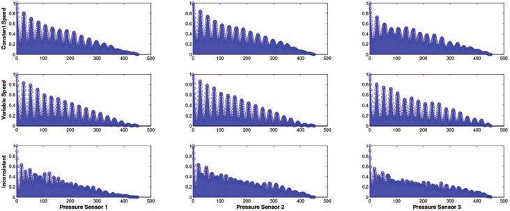
8.2. Analysis
8.2.1. Spatiotemporal. For each experiment we computed the auto-correlation of the
pressure signals within the time window of a segment. The results show that the
correlation in the signals acquired during inconsistent walking degrade more rapidly
compared to those during constant speed and variable speed segments. Figure 13 shows
the results of the auto-correlation for three different pressure sensors on the left foot.
ACM Transactions on Embedded Computing Systems, Vol. 12, No. 1s, Article 57, Publication date: March 2013.HERMES: Mobile System for Instability Analysis and Balance Assessment 57:19 Fig. 13. The auto correlation of 3 pressure sensors is calculated across three different patterns of walking. This result shows how the correlation of the signal in the inconsistent ambulation degrades rapidly compared to normal walking. Fig. 14. This figure shows the swing, stance and dual stance features. For constant speed (left column), it is again apparent that the features remain fairly constant. For gradual speed change (middle column), we see a more downward linear trend than for the stance phase. This is indicative of the user increasing their speed over time, this is due to the change in overall swing to stance ratio. Inconsistent walking patterns (right column)again demonstrate a relatively high variance. 8.2.2. Temporal. A total of six temporal features were extracted as described in Section 5. Figure 14 plots the feature over time for the three different cases. First thing to note is the high variability in the feature for the inconsistent case relative to the two normal patterns. The variable speed graph also shows the need to consider trend in calculating the variance; the fact that the person slows down should not affect their instability as it can be seen by the low variability around the trend. 8.2.3. Variance. Trend and variances were also computed for the temporal parameters across all three patterns. Hermes is able to compute the variance of each of the detected features by isolating the variability of the feature signal by taking the signals’ ACM Transactions on Embedded Computing Systems, Vol. 12, No. 1s, Article 57, Publication date: March 2013.
57:20                                                                                           H. Noshadi et al.

Fig. 15. The trend and variance is calculated across three patterns of walking: constant speed, gradual
speed change, and inconsistent walking. By removing the trend from the original signal we are able to
isolate the variability of the signal but calculating the variance of the resulting signal. std(const speed)=1.43,
std(gradual change)=1.74, and std(inconsistent)=3.76.

                                     Table I. Variance of Temporal Features
                             Feature          Normal     Variable Speed      Inconsistent
                          Stance Left          1.43           1.74               3.78
                         Stance Right          1.48           1.78               4.03
                           Swing Left          0.97           1.12               1.75
                          Swing Right          1.06           1.04               1.63
                         S/R Ratio Left        0.04           0.05               0.08
                        S/R Ratio Right        0.38           0.05               0.08
                          Dual Stance          0.55           0.88               1.26
                           Stride Left         2.07           2.28               7.08
                          Stride Right         2.12           2.29               6.95
                            Step Left          1.24           1.57               2.25
                           Step Right          1.39           1.62               2.76

trend into the consideration. Figure 15 illustrates how this is done for the stance time.
First the trend line is determined for the segment as shown in the left graphs. Then
the trend is removed from the signal, as shown by the right graphs from which the
variance is calculated.
   We aggregated the variability of the features extracted for all subjects, where the
resulting variances are shown in Table I. The table contains the corresponding variabil-
ity analysis of the temporal features for each of the targeted ambulation patterns for
12 subjects. As table suggests the difference between variability of features in normal
and variable speed walk is much less than the variability between normal and incon-
sistent walk. This suggests that even though variable speed walk will result in higher
variance of features, however it is not comparable with the increase of the variability
in the inconsistent case.

          ACM Transactions on Embedded Computing Systems, Vol. 12, No. 1s, Article 57, Publication date: March 2013.
You can also read