Federal Reserve Bank of Minneapolis - The Great Depression in the United States From a Neoclassical Perspective (p. 2)
←
→
Page content transcription
If your browser does not render page correctly, please read the page content below
Federal Reserve Bank
                   of Minneapolis

i;

     Winter 1999

                   The Great Depression
                   in the United States
                   From a Neoclassical
                   Perspective (p. 2)
                   Harold L. Cole
                   Lee E. Ohanian

                   Some Observations on the
                   Great Depression (p. 25)
                   Edward C. Prescott

                   1998 Contents (p. 32)

                   1998 Staff Reports (p. 33)
Federal Reserve Bank of Minneapolis

Quarterly ReviewVol.23,No.1
ISSN 0271-5287

This publication primarily presents economic research aimed
at improving policymaking by the Federal Reserve System and
other governmental authorities.

Any views expressed herein are those of the authors and
not necessarily those of the Federal Reserve Bank of Minneapolis
or the Federal Reserve System.

                    Editor: Arthur J. Rolnick
       Associate Editors: Edward J. Green, Preston J. Miller,
                            Warren E. Weber
Economic Advisory Board: Harold L. Cole, Edward J. Green,
                            Lee E. Ohanian, James A. Schmitz, Jr.
        Managing Editor: Kathleen S. Rolfe
            Article Editor: Jenni C. Schoppers
                 Designer: Phil Swenson
                Typesetter: Mary E. Anomalay
    Circulation Assistant: Elaine R. Reed

The Quarterly Review is published by the Research Department           Comments and questions about the Quarterly Review may be
of the Federal Reserve Bank of Minneapolis. Subscriptions are          sent to
available free of charge.                                              Quarterly Review
Quarterly Review articles that are reprints or revisions of papers     Research Department
published elsewhere may not be reprinted without the written           Federal Reserve Bank of Minneapolis
permission of the original publisher. All other Quarterly Review       P.O. Box 291
articles may be reprinted without charge. If you reprint an article,   Minneapolis, Minnesota 55480-0291
please fully credit the source—the Minneapolis Federal Reserve         (Phone 612-204-6455 / Fax 612-204-5515).
Bank as well as the Quarterly Review—and include with the              Subscription requests may also be sent to the circulation
reprint a version of the standard Federal Reserve disclaimer           assistant at elaine.reed@mpls.frb.org; editorial comments and
(italicized above). Also, please send one copy of any publication      questions, to the managing editor at ksr@res.mpls.frb.fed.us.
that includes a reprint to the Minneapolis Fed Research
Department.
Electronicfiles of Quarterly Review articles are available through
the Minneapolis Fed's home page on the World Wide Web:
http://www.mpls.frb.org.
Federal Reserve Bank of Minneapolis
     Quarterly Review Winter 1999

     The Great Depression in the United States
     From a Neoclassical Perspective*

     Harold L. Cole                         Lee E. Ohaniant
     Senior Economist                       Economist
     Research Department                    Research Department
     Federal Reserve Bank of Minneapolis    Federal Reserve Bank of Minneapolis

Between 1929 and 1933, employment fell about 25 per-           work, can account for the decline and the recovery in the
cent and output fell about 30 percent in the United States.    1930s. This method allows us to understand which data
By 1939, employment and output remained well below             from the 1930s are consistent with neoclassical theory and,
their 1929 levels. Why did employment and output fall so       especially, which observations are puzzling from the neo-
much in the early 1930s? Why did they remain so low a          classical perspective.
decade later?                                                     In our analysis, we treat the 1929-33 decline as a long
   In this article, we address these two questions by eval-    and severe recession.2 But the neoclassical approach to an-
uating macroeconomic performance in the United States          alyzing business cycles is not just to assess declines in eco-
from 1929 to 1939. This period consists of a decline in eco-   nomic activity, but to assess recoveries as well. When we
nomic activity (1929-33) followed by a recovery (1934-         compare the decline and recovery during the Depression to
39). Our definition of the Great Depression as a 10-year       a typical postwar business cycle, we see striking differ-
event differs from the standard definition of the Great De-
pression, which is the 1929-33 decline. We define the De-
pression this way because employment and output re-
mained well below their 1929 levels in 1939.                        *The authors acknowledge the tremendous contribution Edward Prescott made to
   We examine the Depression from the perspective of           this project in the many hours he spent talking with them about the Depression and in
                                                               the input and guidance he generously provided. The authors also thank Andy Atkeson,
neoclassical growth theory. By neoclassical growth theory;     Russell Cooper, Ed Green, Chris Hanes, Patrick Kehoe, Narayana Kocherlakota, Art
we mean the optimal growth model in Cass 1965 and              Rolnick, and Jim Schmitz for comments. The authors also thank Jesus Femandez-
                                                               Villaverde for research assistance and Jenni Schoppers for editorial assistance; both
Koopmans 1965 augmented with various shocks that cause         contributed well beyond the call of duty.
employment and output to deviate from their deterministic           tOhanian is also an associate professor of economics at the University of Min-
steady-state paths as in Kydland and Prescott 1982.1           nesota.
                                                                    1 For other studies of the Depression and many additional references, see Brunner
   We use neoclassical growth theory to study macroeco-         1981; Temin 1989, 1993; Eichengreen 1992; Calomiris 1993; Margo 1993; Romer
nomic performance during the 1930s the way other econ-          1993; Bernanke 1995; Bordo, Erceg, and Evans 1996; and Crucini and Kahn 1996.
omists have used the theory to study postwar business cy-           2The National Bureau of Economic Research (NBER) defines a cyclical decline,
                                                               or recession, as a period of decline in output across many sectors of the economy which
cles. Wefirst identify a set of shocks considered important    typically lasts at least six months. Since the NBER uses a monthly frequency, we con-
in postwar economic declines: technology shocks, fiscal        vert to a quarterly frequency for our comparison by considering a peak (trough) quarter
policy shocks, trade shocks, and monetary shocks. We then      to be the quarter with the highest (lowest) level of output within one quarter of the
                                                               quarter that contains the month of the NBER peak (trough). We define the recovery as
ask whether those shocks, within the neoclassical frame-       the time it takes for output to return to its previous peak.

2,
Harold L. Cole, Lee E. Ohanian
  The Great Depression

ences in duration and scale. The decline, as well as the re-
covery, during the Depression lasted about four times as       Table 1
long as the postwar business cycle average. Moreover, the      Duration and Scale of the Depression
size of the decline in output in the 1930s was about 10        and Postwar Business Cycles
times the size of the average decline. (See Table 1.)          Measured by the Decline and Recovery of Output
    What factors were responsible for these large differ-
ences in the duration and scale of the Depression? One
possibility is that the shocks—the unexpected changes in                                               Length                Size of          Length of
technology, preferences, endowments, or government pol-                                              of Decline              Decline          Recovery
icies that lead output to deviate from its existing steady-
state growth path—were different in the 1930s. One view        Great Depression                       4 years              -31.0%              7 years
is that the shocks responsible for the 1929-33 decline were
much larger and more persistent versions of the same           Postwar Cycle Average                  1 year                 -2.9%           1.5 years
shocks that are important in shorter and milder declines.
Another view is that the types of shocks responsible for the
 1929-33 decline were fundamentally different from those       Sources: National Bureau of Economic Research; U.S. Department of Commerce,

considered to be the driving factors behind typical cyclical            Bureau of Economic Analysis

declines.
    To evaluate these two distinct views, we analyze data
from the 1930s using the neoclassical growth model. Our        have led employment and output to return to trend by
mainfinding differs from the standard view that the most       1939.
puzzling aspect of the Depression is the large decline be-         We next analyze whether monetary shocks can account
tween 1929 and 1933. Wefind that while it may be pos-          for the decline and recovery. Some economists, such as
sible to account for the 1929-33 decline on the basis of the   Friedman and Schwartz (1963), argue that monetary shocks
shocks we consider, none of those shocks can account for       were a key factor in the 1929-33 decline. To analyze the
the 1934-39 recovery. Theory predicts large increases in       monetary shock view, we use the well-known model of
employment and output beginning in 1934 that return real       Lucas and Rapping (1969), which connects changes in the
economic activity rapidly to trend. This prediction stands     money supply to changes in output through intertemporal
in sharp contrast to the data, suggesting to us that we need   substitution of leisure and unexpected changes in wages.
a new shock to account for the weak recovery.                  The Lucas-Rapping model predicts that monetary shocks
    We begin our study by examining deviations in output       reduced output in the early 1930s, but the model also pre-
and inputs from the trend growth that theory predicts in the   dicts that employment and output should have been back
absence of any shocks to the economy. This examination         near trend by the mid-1930s.
not only highlights the severity of the economic decline           Both real shocks and monetary shocks predict that em-
between 1929 and 1933, but also raises questions about the     ployment and output should have quickly returned to trend
recovery that began in 1934. In 1939, real per capita output   levels. These predictions are difficult to reconcile with the
remained 11 percent below its 1929 level: output increases     weak 1934-39 recovery. If the factors considered impor-
an average of 21 percent during a typical 10-year period.      tant in postwarfluctuations can't fully account for macro-
This contrast identifies two challenges for theory: account-   economic performance in the 1930s, are there other factors
ing for the large decline in economic activity that occurred   that can? We go on to analyze two other factors that some
between 1929 and 1933 and accounting for the weak re-          economists consider important in understanding the De-
covery between 1934 and 1939.                                  pression:financial intermediation shocks and inflexible
    Wefirst evaluate the importance of real shocks—tech-       nominal wages. One type of financial intermediation shock
nology shocks,fiscal policy shocks, and trade shocks—for       is the bank failures that occurred during the early 1930s.
this decade-long period. Wefind that technology shocks         Some researchers argue that these failures reduced output
may have contributed to the 1929-33 decline. However,          by disruptingfinancial intermediation. While bank failures
wefind that the real shocks predict a very robust recovery     perhaps deepened the decline, we argue that their impact
beginning in 1934. Theory suggests that real shocks should     would have been short-lived and, consequently, that bank

                                                                                                                                                          3
failures were not responsible for the weak recovery. An-                  Output
                                                            In Table 2, we compare levels of output during the De-
other type of financial intermediation shock is the increases
in reserve requirements that occurred in late 1936 and earlypression to peak levels in 1929. To do this, we present data
 1937. While this change may have led to a small decline    on consumption and investment and the other components
in output in 1937, it cannot account for the weak recovery  of real gross national product (GNP) for the 1929-39 pe-
prior to 1937 and cannot account for the significant drop   riod.4 Data are from the national income and product ac-
in activity in 1939 relative to 1929.                       counts published by the Bureau of Economic Analysis of
                                                            the U.S. Department of Commerce. All data are divided by
    The other alternative factor is inflexible nominal wages.
The view of this factor holds that nominal wages were not   the working-age (16 years and older) population. Since
as flexible as prices and that the fall in the price level  neoclassical growth theory indicates that these variables
raised real wages and reduced employment. We present        can be expected to grow, on average, at the trend rate of
data showing that manufacturing real wages rose consis-     technology, they are also detrended, that is, adjusted for
tently during the 1930s, but that nonmanufacturing wages    trend growth.5 With these adjustments, the data can be di-
fell. The 10-year increase in manufacturing wages is dif-   rectly compared to their peak values in 1929.
ficult to reconcile with nominal wage inflexibility, which       As we can see in Table 2, all the components of real
typically assumes that inflexibility is due to either money output (GNP in base-year prices), except government pur-
illusion or explicit nominal contracts. The long duration ofchases of goods and services, fell considerably during the
the Depression casts doubt on both of these determinants     1930s. The general pattern for the declining series is a
of inflexible nominal wages.                                very large drop between 1929 and 1933 followed by only
    The weak recovery is a puzzle from the perspective of   a moderate rise from the 1933 trough. Output fell more
neoclassical growth theory. Our inability to account for thethan 38 percent between 1929 and 1933. By 1939, output
recovery with these shocks suggests to us that an alterna-  remained nearly 27 percent below its 1929 detrended lev-
tive shock is important for understanding macroeconomic     el. This detrended decline of 27 percent consists of a raw
performance after 1933. We conclude our study by con-        11 percent drop in per capita output and a further 16 per-
jecturing that government policies toward monopoly and      cent drop representing trend growth that would have nor-
the distribution of income are a good candidate for this    mally occurred over the 1929-39 period.6
shock. The National Industrial Recovery Act (NIRA) of            The largest decline in economic activity occurred in
 1933 allowed much of the economy to cartelize. This pol-   business investment, which fell nearly 80 percent between
icy change would have depressed employment and output        1929 and 1933. Consumer durables, which represent
in those sectors covered by the act and, consequently, have household, as opposed to business, investment, followed
led to a weak recovery. Whether the NIRA can quantita-      a similar pattern, declining more than 55 percent between
tively account for the weak recovery is an open question     1929 and 1933. Consumption of nondurables and services
for future research.                                        declined almost 29 percent between 1929 and 1933. For-
                                                            eign trade (exports and imports) also fell considerably be-
The Data Through the Lens of the Theory                     tween 1929 and 1933. The impact of the decline between
Neoclassical growth theory has two cornerstones: the ag- 1929 and 1933 on government purchases was relatively
gregate production technology, which describes how labor mild, and government spending even rose above its trend
and capital services are combined to create output, and the level in 1930 and 1931.
willingness and ability of households to substitute com-
modities over time, which govern how households allocate
their time between market and nonmarket activities and           3Note that in the closed economy framework of the neoclassical growth model,
how households allocate their income between consump- savings equals investment.
tion and savings. Viewed through the lens of this theory,        4 We end our analysis in 1939 to avoid the effects of World War II.
the following variables are keys to understanding macro- growthsWeratemake  the trend adjustment by dividing each variable by its long-run trend
                                                                        relative to the reference date. For example, we divide GNP in 1930 by
economic performance: the allocation of output between 1.019. This number is 1 plus the average growth rate of 1.9 percent over the 1947-97
consumption and investment, the allocation of time (labor forth.
                                                            period and over the 1919-29 period. For 1931, we divide the variable by 1.019and so
input) between market and nonmarket activities, and pro-         6TO obtain this measure, we divide per capita output in 1939 by per capita output
ductivity.3                                                 in 1929 (0.89) and divide the result by 1.01910.

4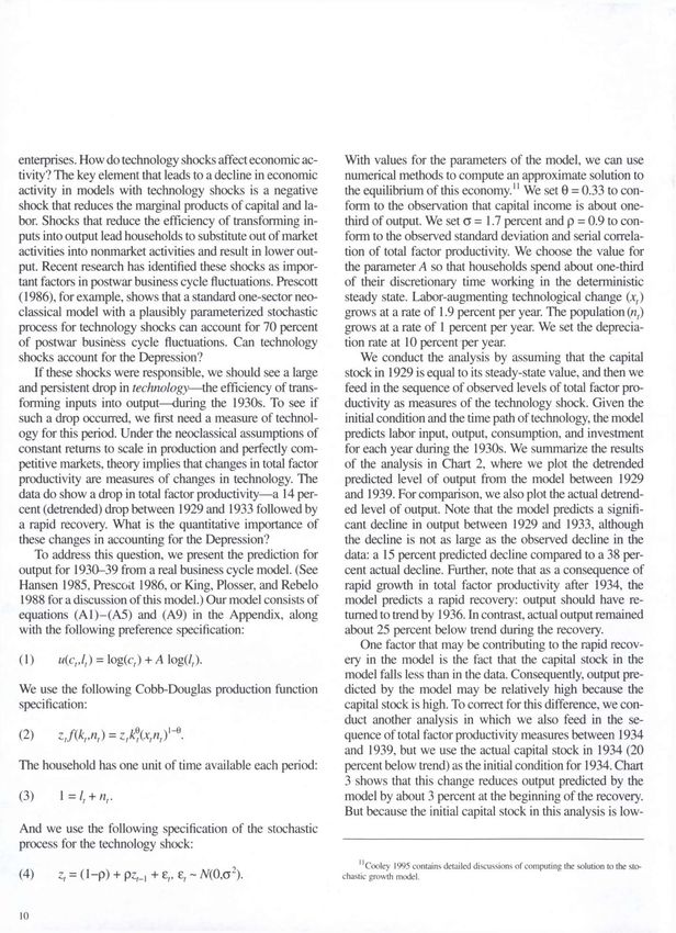
Harold L. Cole, Lee E. Ohanian
    The Great Depression

Table 2
Detrended Levels of Output and Its Components in 1929-39*
Index, 1929=100

                                                                               Consumption
                                         Real                  Nondurables             Consumer      Business     Government         Foreign Trade
            Year                        Output                 and Services            Durables     Investment     Purchases      Exports       Imports

           1930                           87.3                          90.8             76.2         69.2           105.1         85.2          84.9
           1931                           78.0                          85.2             63.3         46.1           105.3         70.5          72.4
           1932                           65.1                          75.8             46.6         22.2           97.2          54.4          58.0
           1933                           61.7                          71.9             44.4         21.8           91.5          52.7          60.7
           1934                           64.4                          71.9             48.8         27.9           100.8         52.7          58.1
           1935                           67.9                          72.9             58.7         41.7           99.8          53.6          69.1
           1936                           74.7                          76.7             70.5         52.6           113.5         55.0          71.7
           1937                           75.7                          76.9             71.9         59.5           105.8         64.1          78.0
           1938                           70.2                          73.9             56.1         38.6           111.5         62.5          58.3
           1939                           73.2                          74.6             64.0         49.0           112.3         61.4          61.3

*Data are divided by the working-age (16 years and older) population.
 Source: U.S. Department of Commerce, Bureau of Economic Analysis

    Table 2 also makes clear that the economy did not re-                                         of output devoted to investment averaged about 15 percent,
cover much from the 1929-33 decline. Although invest-                                             compared to its postwar average of 20 percent. This low
ment improved relative to its 1933 trough level, investment                                       rate of investment led to a decline in the capital stock—the
remained 51 percent below its 1929 (detrended) level in                                           gross stock of fixed reproducible private capital declined
1939. Consumer durables remained 36 percent below their                                           more than 6 percent between 1929 and 1939, representing
1929 level in 1939. Relative to trend, consumption of non-                                        a decline of more than 25 percent relative to trend. Foreign
durables and services increased very little during the re-                                        trade comprised a small share of economic activity in the
covery. In 1933, consumption was about 28 percent below                                           United States during the 1929-39 period. Both exports and
its 1929 detrended level. By 1939, consumption remained                                           imports accounted for about 4 percent of output during the
about 25 percent below this level.                                                                decade. The increase in government purchases, combined
    These unique and large changes in economic activity                                           with the decrease in output, increased the government's
during the Depression also changed the composition of                                             share of output from 13 percent to about 20 percent by
output—the shares of output devoted to consumption, in-                                           1939.
vestment, government purchases, and exports and imports.                                             These data raise the possibility that the recovery was a
These data are presented in Table 3. The share of output                                          weak one. To shed some light on this possibility, in Table
consumed rose considerably during the early 1930s, while                                          4, we show the recovery from a typical postwar recession.
the share of output invested, including consumer durables,                                        The data in Table 4 are average detrended levels relative
declined sharply, falling from 25 percent in 1929 to just 8                                       to peak measured quarterly from the trough. A comparison
percent in 1932. During the 1934-39 recovery, the share                                           of Tables 2 and 4 shows that the recovery from a typical

                                                                                                                                                          5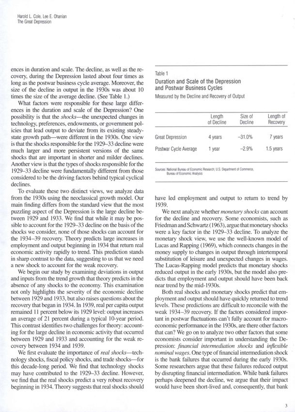
Table 3
Changes in the Composition of Output in 1929-39

                                                                                  Shares of Output

                                                                                                                 Foreign Trade
                                                                         Government
                                   Year                  Consumption     Investment     Purchases          Exports           Imports

                                   1929                            .62      .25            .13                .05               .04
                                   1930                            .64      .19            .16                .05               .04
                                   1931                            .67      .15            .18                .05               .04
                                   1932                            .72      .08            .19                .04               .04
                                   1933                            .72      .09            .19                .04               .04
                                   1934                            .69      .11            .20                .04               .04
                                   1935                            .66      .15            .19                .04               .04
                                   1936                            .63      .17            .20                .04               .04
                                   1937                            .63      .19            .18                .04               .04
                                   1938                            .65      .14            .21                .04               .04
                                   1939                            .63      .16            .20                .04               .04

                                   Postwar Average                          .20            .23                .06               .07
                                                              CO
                                                              en

Source: U.S. Department of Commerce, Bureau of Economic Analysis

postwar recession differs considerably from the 1934-39                               growth path, but was settling on a considerably lower
recovery during the Depression. First, output rapidly re-                             steady-state growth path.
covers to trend following a typical postwar recession. Sec-                              The possibility that the economy was converging to a
ond, consumption grows smoothly following a typical                                   lower steady-state growth path is consistent with the fact
postwar recession. This contrasts sharply to theflat time                             that consumption fell about 25 percent below trend by
path of consumption during the 1934-39 recovery. Third,                               1933 and remained near that level for the rest of the de-
investment recovers very rapidly following a typical post-                            cade. (See Chart 1.) Consumption is a good barometer of
war recession. Despite falling much more than output dur-                             a possible change in the economy's steady state because
ing a recession, investment recovers to a level comparable                            household dynamic optimization implies that all future ex-
to the output recovery level within three quarters after the                          pectations of income should be factored into current con-
trough. During the Depression, however, the recovery in                               sumption decisions.7
investment was much slower, remaining well below the                                  Labor Input
recovery in output.                                                                   Data on labor input are presented in Table 5. We use
   Tables 2 and 4 indicate that the 1934-39 recovery was                              Kendrick's (1961) data on labor input, capital input, pro-
much weaker than the recovery from a typical recession.
One interpretation of the weak 1934-39 recovery is that
the economy was not returning to its pre-1929 steady-state                               7This point isfirst stressed in Hall 1978.

6
Harold L. Cole, Lee E. Ohanian
    The Great Depression

Table 4                                                                             Chart 1
Detrended Levels of Output and Its Components                                       Convergence to a New Growth Path?
in a Typical Postwar Recovery                                                       Detrended Levels
Measured Quarterly From Trough, Peak=100                                            of Consumption and Output
                                                                                    in 1929-39

 Quarters                                                              Government
From Trough          Output        Consumption            Investment    Purchases

      0                95.3              96.8                 84.5        98.0
      1                96.2              98.1                 85.2        97.9
      2                98.3              99.5                 97.3        98.0
      3               100.2             100.8                104.5        99.0
      4               102.1             102.7                112.1        99.2

Source: U.S. Department of Commerce, Bureau of Economic Analysis                    Source: U.S. Department of Commerce, Bureau of Economic Analysis

ductivity, and output.8 We presentfive measures of labor about 1.8 percent per year. In contrast to the other mea-
input, each divided by the working-age population. We sures of labor input, farm hours remained near trend during
don't detrend these ratios because theory implies that they much of the decade. Farm hours were virtually unchanged
will be constant along the steady-state growth path.9 Here, between 1929 and 1933, a period in which hours worked
again, data are expressed relative to their 1929 values.       in other sectors fell sharply. Farm hours did fall about 10
    The three aggregate measures of labor input declined percent in 1934 and were about 7 percent below their 1929
sharply from 1929 to 1933. Total employment, which con- level by 1939. A very different picture emerges for manu-
sists of private and government workers, declined about 24 facturing hours, which plummeted more than 40 percent
percent between 1929 and 1933 and remained 18 percent between 1929 and 1933 and remained 22 percent below
below its 1929 level in 1939. Total hours, which reflect their detrended 1929 level at the end of the decade.
changes in employment and changes in hours per worker,            These data indicate important differences between the
declined more sharply than total employment, and the farm and manufacturing sectors during the Depression.
trough didn't occur until 1934. Total hours remained 21 Why didn't farm hours decline more during the Depres-
percent below their 1929 level in 1939. Private hours, sion? Why did manufacturing hours decline so much?
which don't include the hours of government workers, de-          Finally, note that the changes in nonfarm labor input are
clined more sharply than total hours, reflecting the fact that similar to changes in consumption during the 1930s. In
government employment did not fall during the 1930s. particular, after falling sharply between 1929 and 1933,
Private hours fell more than 25 percent between 1929 and measures of labor input remained well below 1929 levels
1939.                                                          in 1939. Thus, aggregate labor input data also suggest that
    These large declines in aggregate labor input reflect the economy was settling on a growth path lower than the
different changes across sectors of the economy. Farm path the economy was on in 1929.
hours and manufacturing hours are shown in the last two
columns of Table 5. In addition to being divided by the           8Kendrick's (1961) data for output are very similar to those in the NIPA.
working-age population, the farm hours measure is adjust-         9Hours will be constant along the steady-state growth path if preferences and tech-
ed for an annual secular decline in farm employment of nology satisfy certain properties. See King, Plosser, and Rebelo 1988.

                                                                                                                                                       7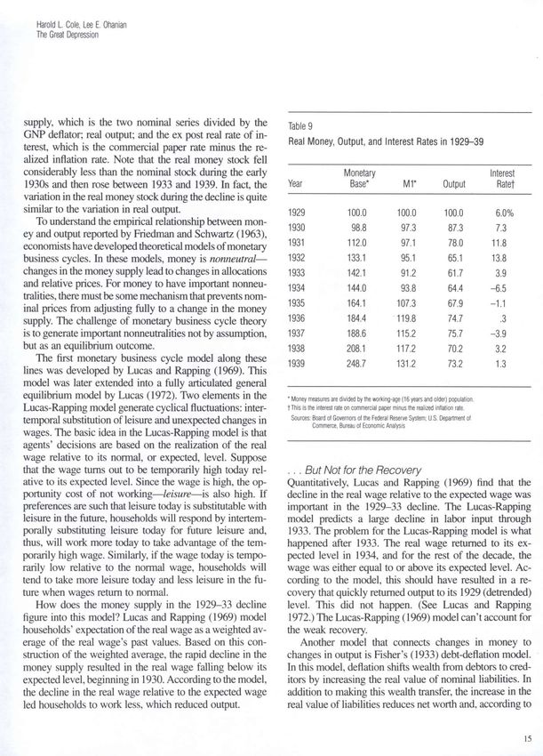
Productivity                                                   long-run path of productivity, why would the economy be
In Table 6, we present two measures of productivity: labor on a lower steady-state growth path in 1939?
productivity (output per hour) and total factor productivity.
Both measures are detrended and expressed relative to An International Comparison
1929 measures. These two series show similar changes Many countries suffered economic declines during the
during the 1930s. Labor productivity and total factor pro- 1930s; however, there are two important distinctions be-
ductivity both declined sharply in 1932 and 1933, falling tween economic activity in the United States and other
about 12 percent and 14 percent, respectively, below their countries during the 1930s. The decline in the United
1929 detrended levels. After 1933, however, both mea- States was much more severe, and the recovery from the
sures rose quickly relative to trend and, in fact, returned to decline was weaker. To see this, we examine average real
trend by 1936. When we compare 1939 data to 1929 data, per capita output relative to its 1929 level for Belgium,
we see that the 1930s were a decade of normal productivi- Britain, France, Germany, Italy, Japan, and Sweden. The
ty growth. Labor productivity grew more than 22 percent data are from Maddison 1991 and are normalized for each
between 1929 and 1939, and total factor productivity grew country so that per capita output is equal to 100 in 1929.
more than 20 percent in the same period. This normal Since there is some debate over the long-run growth rate
growth in productivity raises an important question about in some of these countries, we have not detrended the data.
the lack of a recovery in hours worked, consumption, and          Table 7 shows the U.S. data and the mean of the nor-
investment. In the absence of a large negative shift in the malized data for other countries. The total drop in output

Table 5
Five Measures of Labor Input in 1929-39*
Index, 1929=100

                                                                            Aggregate Measures                   Sectoral Measures
                                                              Total                     Total       Private   Farm       Manufacturing
                                     Year                   Employment                  Hours       Hours     Hourst        Hours

                                    1930                         93.2                    91.9        91.5     99.0            84.6
                                    1931                         85.7                    83.5        82.8     101.7           68.7
                                    1932                         77.5                    73.4        72.4     98.7            54.7
                                    1933                         76.2                    72.6        70.8     99.0            58.4
                                    1934                         79.9                    71.7        68.7     89.3            61.2
                                    1935                         81.4                    74.7        71.4     93.3            68.6
                                    1936                         83.9                    80.6        75.8     91.1            79.2
                                    1937                         86.4                    83.0        79.5     99.1            85.3
                                    1938                         80.4                    76.3        71.7     92.7            67.6
                                    1939                         82.1                    78.7        74.4     93.6            78.0

•Data are divided by the working-age (16 years and older) population,
t Farm hours are adjusted for a secular decline in farm employment of about 1.8 percent per year.
  Source: Kendrick 1961

8
Harold L. Cole, Lee E. Ohanian
     The Great Depression

                                                                                    is relatively small in other countries: an 8.7 percent drop
Table 6                                                                             compared to a 33.3 percent drop in the United States. The
Detrended Measures of Productivity                                                  international economies recovered quickly: output in most
Index, 1929=100                                                                     countries returned to 1929 levels by 1935 and was above
                                                                                    those levels by 1938. Employment also generally recov-
                                                                                    ered to its 1929 level by 1938.10
                                          Labor                   Total Factor          While accounting for other countries' economic de-
               Year                    Productivity*              Productivity      clines is beyond the scope of this analysis, we can draw
                                                                                    two conclusions from this comparison. First, the larger de-
               1930                          95.9                      94.8         cline in the United States is consistent with the view that
               1931                          95.4                      93.5         the shocks that caused the decline in the United States
               1932                          90.7                      87.8         were larger than the shocks that caused the decline in the
               1933                          87.9                      85.9         other countries. Second, the weak recovery in the United
                                                                                    States is consistent with the view that the shocks that im-
               1934                          96.7                      92.6
                                                                                    peded the U.S. recovery did not affect most other coun-
               1935                          98.4                      96.6         tries. Instead, the post-1933 shock seems to be largely spe-
               1936                        101.6                       99.9         cific to the United States.
               1937                        100.7                     100.5              The data we've examined so far suggest that inputs and
                                                                                    output in the United States fell considerably during the
               1938                        102.4                     100.3
                                                                                    1930s and did not recover much relative to the increase in
               1939                        104.6                     103.1          productivity. Moreover, the data show that the decline was
                                                                                    much more severe and the recovery weaker in the United
                                                                                    States than in other countries. To account for the decade-
* Labor productivity is defined as output per hour.                                 long Depression in the United States, we conclude that we
 Sources: Kendrick 1961; U.S. Department of Commerce, Bureau of Economic Analysis   should focus on domestic, rather than international, factors.
                                                                                    We turn to this task in the next section.
Table 7
                                                                                    Can Real Shocks Account for the Depression?
                                                                                    Neoclassical theory and the data have implications for the
U.S. vs. International Decline and Recovery                                         plausibility of different sources of real shocks in account-
Annual Real per Capita Output in the 1930s                                          ing for the Depression. Since the decline in output was so
Index, 1929=100                                                                     large and persistent, we will look for large and persistent
                                                                                    negative shocks. We analyze three classes of real shocks
                                                                                    considered important in typical business cycle fluctuations:
                                        United               International          technology shocks,fiscal policy shocks, and trade shocks.
                Year                    States                 Average*
                                                                                    Technology Shocks? Perhaps Initially
                1932                     69.0                   91.3                First we consider technology shocks, defined as any exog-
                                                                                    enous factor that changes the efficiency with which busi-
                1933                     66.7                   94.5                ness enterprises transform inputs into output. Under this
                                                                                    broad definition of technology shocks, changes in produc-
                1935                     76.3                  101.0                tivity reflect not only true changes in technology, but also
                                                                                    such other factors as changes in work rules and practices
                1938                     83.6                  112.4
                                                                                    or government regulations that affect the efficiency of pro-
                                                                                    duction but are exogenous from the perspective of business
* International average includes Belgium, Britain, France,
 Germany, Italy, Japan, and Sweden.
 Source: Maddison 1991                                                                   10The average ratio of employment in 1939 to employment in 1929 was one in
                                                                                    these countries, indicating that employment had recovered.

                                                                                                                                                               9
enterprises. How do technology shocks affect economic ac- With values for the parameters of the model, we can use
tivity? The key element that leads to a decline in economic numerical methods to compute an approximate solution to
activity in models with technology shocks is a negative the equilibrium of this economy.11 We set 9 = 0.33 to con-
shock that reduces the marginal products of capital and la- form to the observation that capital income is about one-
bor. Shocks that reduce the efficiency of transforming in- third of output. We set a = 1.7 percent and p = 0.9 to con-
puts into output lead households to substitute out of market form to the observed standard deviation and serial correla-
activities into nonmarket activities and result in lower out- tion of total factor productivity. We choose the value for
put. Recent research has identified these shocks as impor- the parameter A so that households spend about one-third
tant factors in postwar business cyclefluctuations. Prescott of their discretionary time working in the deterministic
(1986), for example, shows that a standard one-sector neo- steady state. Labor-augmenting technological change (jcf)
classical model with a plausibly parameterized stochastic grows at a rate of 1.9 percent per year. The population (nt)
process for technology shocks can account for 70 percent grows at a rate of 1 percent per year. We set the deprecia-
of postwar business cyclefluctuations. Can technology tion rate at 10 percent per year.
shocks account for the Depression? We conduct the analysis by assuming that the capital
If these shocks were responsible, we should see a large stock in 1929 is equal to its steady-state value, and then we
and persistent drop in technology—the efficiency of trans- feed in the sequence of observed levels of total factor pro-
forming inputs into output—during the 1930s. To see if ductivity as measures of the technology shock. Given the
such a drop occurred, wefirst need a measure of technol- initial condition and the time path of technology, the model
ogy for this period. Under the neoclassical assumptions of predicts labor input, output, consumption, and investment
constant returns to scale in production and perfectly com- for each year during the 1930s. We summarize the results
petitive markets, theory implies that changes in total factor of the analysis in Chart 2, where we plot the detrended
productivity are measures of changes in technology. The predicted level of output from the model between 1929
data do show a drop in total factor productivity—a 14 per- and 1939. For comparison, we also plot the actual detrend-
cent (detrended) drop between 1929 and 1933 followed by ed level of output. Note that the model predicts a signifi-
a rapid recovery. What is the quantitative importance of cant decline in output between 1929 and 1933, although
these changes in accounting for the Depression? the decline is not as large as the observed decline in the
To address this question, we present the prediction for data: a 15 percent predicted decline compared to a 38 per-
output for 1930-39 from a real business cycle model. (See cent actual decline. Further, note that as a consequence of
Hansen 1985, Prescoit 1986, or King, Plosser, and Rebelo rapid growth in total factor productivity after 1934, the
1988 for a discussion of this model.) Our model consists of model predicts a rapid recovery: output should have re-
equations (A1)-(A5) and (A9) in the Appendix, along turned to trend by 1936. In contrast, actual output remained
with the following preference specification: about 25 percent below trend during the recovery.
One factor that may be contributing to the rapid recov-
(1) u(crlt) = \og(ct) + A log(/,). ery in the model is the fact that the capital stock in the
model falls less than in the data. Consequently, output pre-
We use the following Cobb-Douglas production function dicted by the model may be relatively high because the
specification: capital stock is high. To correct for this difference, we con-
duct another analysis in which we also feed in the se-
(2) ztf(krnt) = ztk«(xtnt)l-e. quence of total factor productivity measures between 1934
and 1939, but we use the actual capital stock in 1934 (20
The household has one unit of time available each period: percent below trend) as the initial condition for 1934. Chart
3 shows that this change reduces output predicted by the
(3) 1 =lt + nr model by about 3 percent at the beginning of the recovery.
But because the initial capital stock in this analysis is low-
And we use the following specification of the stochastic
process for the technology shock:
1 'Cooley 1995 contains detailed discussions of computing the solution to the sto-
(4) z, = (1-p) + pzt.{ + e„ £, - W(0,c2). chastic growth model.
10Harold L. Cole, Lee E. Ohanian
The Great Depression
Chart 2 Chart 3
Predicted and Actual Output in 1929-39 Predicted and Actual Recovery of Output in 1934-39
Detrended Levels, With Initial Detrended Levels, With Initial
Capital Stock in the Model Capital Stock in the Model
Equal to the Actual Capital Stock Equal to the Actual Capital Stock
in 1929 in 1934
Source of basic data: U.S. Department of Commerce, Bureau of Economic Analysis Source of basic data: U.S. Department of Commerce, Bureau of Economic Analysis
er, the marginal product of capital is higher, and the pre- percentage change in output minus the percentage change
dicted rate of output growth in the recovery is faster than in inputs, overstating the inputs will understate productivi-
in thefirst analysis. This recovery brings output back to its ty, while understating the inputs will overstate productivi-
trend level by 1937. The predicted output level is about 27 ty. During the 1929-33 decline, some capital was left idle.
percent above the actual data level in 1939.12 Thus, the The standard measure of capital input is the capital stock.
predicted recovery is stronger than the actual recovery be- Because this standard measure includes idle capital, it is
cause predicted labor input is much higher than actual la- possible that capital input was overstated during the de-
bor input. cline and, consequently, that productivity growth was un-
Based on measured total factor productivity during the derstated.13 Although there are no widely accepted mea-
Depression, our analysis suggests a mixed assessment of sures of capital input adjusted for changes in utilization,
the technology shock view. On the negative side, the actual this caveat raises the possibility that the decline in aggre-
slow recovery after 1933 is at variance with the rapid re- gate total factor productivity in the early 1930s partially
covery predicted by the theory. Thus, it appears that some
shock other than to the efficiency of production is impor-
tant for understanding the weak recovery between 1934
and 1939. On the positive side, however, the theory pre- 12Some researchers argue that there are many other forms of capital, such as or-
dicts that the measured drop in total factor productivity can ganizational capital and human capital, and that the compensation of labor also includes
account for about 40 percent of the decline in output be- the implicit compensation of these other types of capital. These researchers argue, there-
fore, that the true capital share is much higher, around two-thirds, and note that with this
tween 1929 and 1933. higher capital share, convergence in the neoclassical model is much slower. To see what
Note, however, one caveat in using total factor pro- a higher capital share would imply for the 1934-39 recovery, we conducted our recov-
ery exercise assuming a capital share of two-thirds rather than one-third. While slower,
ductivity as a measure of technology shocks during pe- the recovery was still much faster than in the data. This exercise predicted output at 90
riods of sharp changes in output, such as the 1929-33 percent of trend by 1936 and at 95 percent of trend by 1939.
decline: An imperfect measurement of capital input can 13Bernanke and Parkinson (1991) estimate returns to scale for some manufacturing
industries during the Depression and alsofind evidence that productivity fell during this
affect measured aggregate total factor productivity. Be- period. They attribute at least some of the decline to mismeasurement of capital input
cause total factor productivity change is defined as the or increasing returns.
11reflects mismeasurement of capital input.14 Without better the view that government purchase shocks were responsi-
data on capital input or an explicit theoretical framework ble for the downturn.15
we can use to adjust observed measured total factor pro- Although changes in government purchases are not
ductivityfluctuations for capital utilization, we can't easily important in accounting for the Depression, the way they
measure how large technology shocks were in the early werefinanced may be. Government purchases are largely
1930s and, consequently, how much of a drop in output financed by distorting taxes—taxes that affect the marginal
technology shocks can account for. conditions of households orfirms. Most government rev-
It is important to note here that these results give us an enue is raised by taxing factor incomes. Changes in factor
important gauge not only for the technology shock view, income taxes change the net rental price of the factor. In-
but also for any other shock which ceased to be operative creases in labor and capital income taxes reduce the returns
after 1933. The predicted rapid recovery in the second ex- to these factors and, thus, can lead households to substitute
periment implies that any shock which ceased to be op- out of taxed activities by working and saving less.
erative after 1933 can't easily account for the weak re- If changes in factor income taxes were a key factor in
covery. the 1930s economy, these rates should have increased con-
siderably in the 1930s. Tax rates on both labor and capital
Fiscal Policy Shocks? A Little changed very little during the 1929-33 decline, but rose
Next we considerfiscal policy shocks—changes in govern- during the rest of the decade. Joines (1981) calculates that
ment purchases or tax rates. Christiano and Eichenbaum between 1929 and 1939, the average marginal tax rate on
(1992) argue that government purchase shocks are impor- labor income increased from 3.5 percent to 8.3 percent and
tant in understanding postwar business cycle fluctuations, the average marginal tax rate on capital income increased
and Braun (1994) and McGrattan (1994) argue that shocks from 29.5 percent to 42.5 percent. How much should these
to distorting taxes have had significant effects on postwar increases have depressed economic activity? To answer
cyclical activity. this question, we consider a deterministic version of the
To understand how government purchases affect eco- model we used earlier to analyze the importance of tech-
nomic activity, consider an unexpected decrease in govern- nology shocks. We augment this model to allow for dis-
ment purchases. This decrease will tend to increase private tortionary taxes on labor and capital income. The values of
consumption and, consequently, lower the marginal rate of the other parameters are the same. We then compare the
substitution between consumption and leisure. Theory pre- deterministic steady state of the model with 1939 tax rates
dicts that this will lead households to work less and take to the deterministic steady state of the model with 1929 tax
more leisure. Conversely, consider an increase in govern- rates. With these differences in tax rates, wefind that
ment purchases. This increase will tend to decrease private steady-state labor input falls by 4 percent. This suggests
consumption and reduce the marginal rate of substitution thatfiscal policy shocks account for only about 20 percent
between consumption and leisure. In this case, theory pre- of the weak 1934-39 recovery.
dicts that this will lead households to work more and take
less leisure.
Historically, changes in government purchases have had
large effects on economic activity. Ohanian (1997) shows 14An extreme approach to evaluating the effects of idle capital on total factor pro-
ductivity measurement is to assume that output is produced from a Leontief technology
that the increase in government purchases during World using capital and labor. Under this Leontief assumption, the percentage decline in capital
War II can account for much of the 60 percent increase in services is equal to the percentage decline in labor services. Total hours drop 27.4 per-
cent between 1929 and 1933. Under the Leontief assumption, total factor productivity
output during the 1940s. Can changes in government pur- in 1933 is about 7 percent below trend, compared to the 14 percent decline under the
chases also account for the decrease in output in the 1930s? opposite extreme view that all capital is utilized. This adjustment from a 14 percent de-
cline to a 7 percent decline is almost surely too large not only because it is based on a
If government purchase shocks were a key factor in the Leontief technology, but also because it does not take into account the possibility that
decline in employment and output in the 1930s, govern- the capital left idle during the decline was of lower quality than the capital kept in op-
eration.
ment purchases should have declined considerably during l5One reason that private investment may have fallen in the 1930s is because gov-
the period. This did not occur. Government purchases de- ernment investment was substituting for private investment; however, this seems un-
clined modestly between 1929 and 1933 and then rose likely. Government investment that might be a close substitute for private investment did
not rise in the 1930s: government expenditures on durable goods and structures were 3
sharply during the rest of the decade,risingabout 12 per- percent of output in 1929 andfluctuated between 3 percent and 4 percent of output dur-
cent above trend by 1939. These data are inconsistent with ing the 1930s.
12Harold L. Cole, Lee E. Ohanian
The Great Depression
Trade Shocks? No goods are poor substitutes. In this case, tariffs provide little
Finally, we consider trade shocks. In the late 1920s and benefit to domestic producers and, in fact, can even hurt
early 1930s, tariffs—domestic taxes on foreign goods— domestic producers if there are sufficient complementari-
rose in the United States and in other countries. Tariffs ties between inputs. This suggests that tariffs would not be
raise the domestic price of foreign goods and, consequent- used much if substitution elasticities were very low.
ly, benefit domestic producers of goods that are substitutes But even if substitution elasticities were low, it is un-
with the taxed foreign goods. Theory predicts that in- likely that this factor was responsible for the Depression,
creases in tariffs lead to a decline in world trade. Interna- because the rise in the prices of tariffed goods would ul-
tional trade did, indeed, fall considerably during the 1930s: timately have led domestic producers to begin producing
the League of Nations (1933) reports that world trade fell the imported inputs. Once these inputs became available
about 65 percent between 1929 and 1932. Were these tariff domestically, the decline in output created by the tariff
increases responsible for the 1929-33 decline? would have been reversed. It is hard to see how the dis-
To address this question, wefirst study how a contrac- ruption of trade could have affected output significantly for
tion of international trade can lead to a decline in output. more than the presumably short period it would have taken
In the United States, trade is a small fraction of output and domestic producers to change their production.
is roughly balanced between exports and imports. Lucas Our analysis thus far suggests that none of the real
(1994) argues that a country with a small trade share will shocks usually considered important in understanding busi-
not be affected much by changes in trade. Based on the ness cyclefluctuations can account for macroeconomic
small share of trade at the time, Lucas (1994, p. 13) argues performance during the 1930s. Lacking an understanding
that the quantitative effects of the world trade contraction of the Depression based on real shocks, we next examine
during the 1930s are likely to have been "trivial."16 the effects of monetary shocks from the neoclassical per-
Can trade have an important effect even if the trade spective.
share is small? Crucini and Kahn (1996) argue that a sig- Can Monetary Shocks Account
nificant fraction of imports during the 1930s were inter- for the Depression?
mediate inputs. If imported intermediate inputs are imper- Monetary
fect substitutes with domestic intermediate inputs, produc- money—areshocks—unexpected changes in the stock of
tion can fall as a result of a reduction in imported inputs. understanding business cycles, and manytoeconomists
considered an alternative real shocks for
think
Quantitatively, the magnitude of the fall is determined by monetary shocks were a key factor in the 1929-33 decline.
the elasticity of substitution between the inputs. If the Much of the attraction to monetary shocks as a source of
goods are poor substitutes, then a reduction in trade can business cycles comes from the influential narrative mone-
have sizable effects. Little information is available regard- tary history of the United States by Friedman and Schwartz
ing the substitution elasticity between these goods during
the Depression. The preferred estimates of this elasticity
in the postwar United States are between one and two.
(See Stern, Francis, and Schumacher 1976.) Crucini and 16TO understand why a trade disruption would have such a small effect on output
Kahn (1996) assume an elasticity of two-thirds and report in a country with a small trade share, consider the following example. Assume that fina
that output would have dropped about 2 percent during goods are produced with both domestic (Z) and foreign (M) intermediate goods and that
the early 1930s as a result of higher tariffs. the prices of all goods are normalized to one. Assuming an elasticity of substitution be-
tween home and foreign goods of one implies that the production for final goods, Y,
This small decline implies that extremely low substitu- Cobb-Douglas, or
tion elasticities are required if the trade disruption is to r=z A/'-
a a
account for more than a small fraction of the decline in
output. How plausible are very low elasticities? The fact with where a is the share parameter for intermediate inputs. This assumption implies that
the level of domestic intermediate goods held fixed,
that tariffs were widely used points to high, rather than
low, elasticities between inputs. To see this, note that with %AY= (\-a)%AM.
high elasticities, domestic and foreign goods are very good That fact that U.S. imports were 4 percent of total output and U.S. exports 5 percent in
substitutes, and, consequently, tariffs should benefit domes- 1929 suggests that the highest the cost share of inputs in production could have been is
tic producers who compete with foreign producers. With 0.04/0.95 - 0.04. Hence, an extreme disruption in trade that led to an 80 percent drop
in imports would lead to only a 3.2 percent drop in output. (See Crucini and Kahn 1996
very low elasticities, however, domestic goods and foreign for more on this issue.)
13Table 8
Nominal Money, Prices, and Interest Rates in 1929-39 i
Annual % Interest Rate
Monetary Price 3-Month Commercial
Year Base*
Mr Level U.S. T-Bill Paper
1929 100.0 100.0 100.0 4.4% 6.1%
1930 95.9 94.4 97.0 2.2 4.3
1931 98.7 85.6 88.1 1.2 2.6
1932 104.3 74.5 78.4 .8 2.7
1933 108.9 69.9 76.7 .3 1.7
1934 119.8 78.0 83.2 .3 2.0
1935 139.2 91.0 84.8 .2 .8
1936 157.2 102.1 85.2 .1 .8
1937 168.5 102.9 89.4 .5 .9
1938 181.5 102.2 87.2 .1 .8
1939 215.5 113.7 86.6 .0 .6
*Money measures are divided by the working-age (16 years and older) population.
Source: Board of Governors of the Federal Reserve System
(1963). They present evidence that declines in the money In Table 8, we present the nominal data: the monetary
supply tend to precede declines in output over nearly a base, which is the monetary aggregate controlled by the
century in the United States. They also show that the mon- Federal Reserve; M1, which is currency plus checkable de-
ey supply fell sharply during the 1929-33 decline. Fried- posits; the GNP deflator, or price level; and two interest
man and Schwartz (1963, pp. 300-301) conclude from rates: the rate on three-month U.S. Treasury bills and the
these data that the decline in the money supply during the rate on commercial paper. The money supply data are ex-
1930s was an important cause of the 1929-33 decline pressed in per capita terms by dividing by the working-age
(contraction): population. The money data are also expressed relative to
The contraction is in fact a tragic testimonial to the impor- their 1929 values. The interest rates are the annual average
tance of monetary forces . . . . Prevention or moderation of percentage rates. These nominal data do, indeed, show the
the decline in the stock of money, let alone the substitution of large decline in Ml in the early 1930s that led Friedman
monetary expansion, would have reduced the contraction's and Schwartz (1963) to conclude that the drop in the mon-
severity and almost as certainly its duration. ey supply was an important cause of the 1929-33 de-
cline.17
Maybe for the Decline ...
We begin our discussion of the monetary shock view of In Table 9, we present the real data: the real money
the decline by presenting data on some nominal and real
variables. We present the data Friedman and Schwartz
(1963) focus on: money, prices, and output. We also pre- l7Note that the monetary base, which is the components of Ml controlled by the
sent data on interest rates. Federal Reserve, grew between 1929 and 1933.
14Harold L. Cole, Lee E. Ohanian
The Great Depression
supply, which is the two nominal series divided by the Table 9
GNP deflator; real output; and the ex post real rate of in-
terest, which is the commercial paper rate minus the re- Real Money, Output, and Interest Rates in 1929-39
alized inflation rate. Note that the real money stock fell
considerably less than the nominal stock during the early Monetary Interest
1930s and then rose between 1933 and 1939. In fact, the Year Base* M1* Output Ratef
variation in the real money stock during the decline is quite
similar to the variation in real output. 1929 100.0 100.0 100.0 6.0%
To understand the empirical relationship between mon-
ey and output reported by Friedman and Schwartz (1963), 1930 98.8 97.3 87.3 7.3
economists have developed theoretical models of monetary 1931 112.0 97.1 78.0 11.8
business cycles. In these models, money is nonneutral— 1932 133.1 95.1 65.1 13.8
changes in the money supply lead to changes in allocations 1933 142.1 91.2 61.7 3.9
and relative prices. For money to have important nonneu- 1934 144.0 64.4
tralities, there must be some mechanism that prevents nom- 93.8 -6.5
inal prices from adjusting fully to a change in the money 1935 164.1 107.3 67.9 -1.1
supply. The challenge of monetary business cycle theory 1936 184.4 119.8 74.7 .3
is to generate important nonneutralities not by assumption, 1937 188.6 115.2 75.7 -3.9
but as an equilibrium outcome. 1938 208.1 117.2 70.2 3.2
Thefirst monetary business cycle model along these
lines was developed by Lucas and Rapping (1969). This 1939 248.7 131.2 73.2 1.3
model was later extended into a fully articulated general
equilibrium model by Lucas (1972). Two elements in the * Money measures are divided by the working-age (16 years and older) population,
Lucas-Rapping model generate cyclicalfluctuations: inter- t This is the interest rate on commercial paper minus the realized inflation rate.
temporal substitution of leisure and unexpected changes in Sources: Board of Governors of the Federal Reserve System; U.S. Department of
wages. The basic idea in the Lucas-Rapping model is that Commerce, Bureau of Economic Analysis
agents' decisions are based on the realization of the real
wage relative to its normal, or expected, level. Suppose
that the wage turns out to be temporarily high today rel- ... But Not for the Recovery
ative to its expected level. Since the wage is high, the op- Quantitatively, Lucas and Rapping (1969)find that the
portunity cost of not working—leisure—is also high. If decline in the real wage relative to the expected wage was
preferences are such that leisure today is substitutable with important in the 1929-33 decline. The Lucas-Rapping
leisure in the future, households will respond by intertem- model predicts a large decline in labor input through
porally substituting leisure today for future leisure and, 1933. The problem for the Lucas-Rapping model is what
thus, will work more today to take advantage of the tem- happened after 1933. The real wage returned to its ex-
porarily high wage. Similarly, if the wage today is tempo- pected level in 1934, and for the rest of the decade, the
rarily low relative to the normal wage, households will wage was either equal to or above its expected level. Ac-
tend to take more leisure today and less leisure in the fu- cording to the model, this should have resulted in a re-
ture when wages return to normal. covery that quickly returned output to its 1929 (detrended)
How does the money supply in the 1929-33 decline level. This did not happen. (See Lucas and Rapping
figure into this model? Lucas and Rapping (1969) model 1972.) The Lucas-Rapping (1969) model can't account for
households' expectation of the real wage as a weighted av- the weak recovery.
erage of the real wage's past values. Based on this con- Another model that connects changes in money to
struction of the weighted average, the rapid decline in the changes in output is Fisher's (1933) debt-deflation model.
money supply resulted in the real wage falling below its In this model, deflation shifts wealth from debtors to cred-
expected level, beginning in 1930. According to the model, itors by increasing the real value of nominal liabilities. In
the decline in the real wage relative to the expected wage addition to making this wealth transfer, the increase in the
led households to work less, which reduced output. real value of liabilities reduces net worth and, according to
15Fisher, leads to lower lending and a higher rate of business nous response to the overall decline in economic activity.19
failures. Qualitatively, Fisher's view matches up with the Moreover, bank failures were common in the United States
1929-32 period, in which both nominal prices and output during the 1920s, and most of those bank failures did not
were falling. The quantitative importance of the debt-defla- seem to have important aggregate consequences. Wicker
tion mechanism for this period, however, is an open ques- (1980) and White (1984) argue that at least some of the
tion. Of course, Fisher's model would tend to predict a failures during the early 1930s were similar to those during
rapid recovery in economic activity once nominal prices the 1920s.
stopped falling in 1933. Thus, Fisher's model can't account However, we can assess the potential contribution of
for the weak recovery either.18 intermediation shocks to the 1929-33 decline with the fol-
lowing growth accounting exercise. We can easily show
that under the assumption of perfect competition, at least
Factors other than those considered important in postwar locally, the percentage change in aggregate output, Y, can
Alternative Factors
business cycles have been cited as important contributors the sector iasoutputs,
be written a linear function of the percentage change in
% for each sector i = 1,..., n and the
to the 1929-33 decline. Do any provide a satisfactory ac- shares y; for each sector as follows:
counting for the Depression from the perspective of neo-
classical theory? We examine two widely cited factors: (5) i> = E,l,YJ,-
financial intermediation shocks and inflexible nominal
wages. The share of the entirefinance, insurance, and real estate
Were Financial Intermediation Shocks Important? (FIRE) sector went from 13 percent in 1929 to 11 percent
• Bank Failures? Maybe, But Only Briefly in 1933. This suggests that the appropriate cost share was
Several economists have argued that the large number of percent 12 percent. The real output of the FIRE sector dropped 39
bank failures that occurred in the early 1930s disrupted fi- exogenous, between 1929 and 1933. If we interpret this fall as
nancial intermediation and that this disruption was a key reduces output we see that the drop in the entire FIRE sector
factor in the decline. Bernanke's (1983) work provides em- large aggregate externalities by 4.7 percent. Thus, in the absence of
pirical support for this argument. He constructs a statistical the contribution of the FIREthat would amplify this effect,
sector was small.20
model, based on Lucas and Rapping's (1969) model, in
which unexpected changes in the money stock lead to
changes in output. Bernanke estimates the parameters of 18In addition to Lucas and Rapping's (1969)findings and Fisher's (1933) debt-
his model using least squares, and he shows that adding the deflation view, we have other reasons to question the monetary shock view of the De-
dollar value of deposits and liabilities of failing banks as pression. During the mid- and late-1930s, business investment remained more than 50
explanatory variables significantly increases the fraction of percent below its 1929 level despite short-term real interest rates (commercial paper)
near zero and long-term real interest rates (Baa corporate bonds) at or below long-run
output variation the model can account for. averages. These observations suggest that some other factor was impeding the recovery.
What economic mechanism might have led bank fail- argues19Bernanke (1983) acknowledges the possibility of an endogenous response but
that it was probably not important, since problems infinancial intermediation
ures to deepen the 1929-33 decline? One view is that these tended to precede the decline in overall activity and because some of the bank failures
failures represented a decline in information capital asso- seemRecent to have been due to contagion or events unrelated to the overall downturn.
work by Calomiris and Mason (1997) raises questions about the view that
ciated with specific relationships between borrowers and bank runs reflected contagion and raises the possibility that productive, as well as un-
intermediaries. Consequently, when a bank failed, this re- productive, banks could be run. Calomiris and Mason analyze the bank panic in Chicago
in June 1932 andfind that most of the failures were among insolvent, or near-insolvent,
lationship-specific capital was lost, and the efficiency of in- banks.
termediation declined. 20TO see how we derive the linear expression for Y, note that if Y - F(yit>>„),
It is difficult to assess the quantitative importance of
bank failures as a factor in deepening the 1929-33 decline then
because the output of the banking sector, like broader mea-
sures of economic activity, is an endogenous, not an ex- Note also that if goods are produced competitively, then the price of each factor / is
by its marginal product F,-. Hence, y, = F,y,/K and the result follows.
ogenous, variable. Although bank failures may have exac- givenNote
erbated the decline, as suggested by Bernanke's (1983) the notionthatthatthetherefactwasthatextremely
the cost shares didn't change very much is inconsistent with
low elasticity of substitution for this input and that
empirical work, some of the decline in the inputs and out- production
the fall in this input was an important cause of the fall in output. For example, a Leontief
put of the banking sector may also have been an endoge- \j would gofunction in which F(y, t v„) = min, v, implies that the cost share of input
to one if that input was the input in short supply.
16You can also read