Analysis of Total Column CO2 and CH4 Measurements in Berlin with WRF-GHG
←
→
Page content transcription
If your browser does not render page correctly, please read the page content below
Analysis of Total Column CO2 and CH4 Measurements in Berlin
     with WRF-GHG
     Xinxu Zhao1 , Julia Marshall2 , Stephan Hachinger3 , Christoph Gerbig2 , Matthias Frey4 , Frank Hase4 , and
     Jia Chen1
     1
       Electrical and Computer Engineering, Technische Unversität München, 80333 Munich, Germany
     2
       Max Plank Institute of Biogeochemistry, 07745 Jena, Germany
     3
       Leibniz Supercomputing Center (Leibniz-Rechenzenturm, LRZ) of Bavarian Academy of Sciences and Humanities,
     Bolzmannstr. 1, 85748 Garching, Germany
     4
       Karlsruhe Institute of Technology (KIT), Institute of Meteorology and Climate Research (IMK-ASF), Karlsruhe, Germany
     Correspondence: Jia Chen (jia.chen@tum.de)

     Abstract. Though they cover less than 3 % of the global land area, urban areas are responsible for over 70 % of the global
     greenhouse gas (GHG) emissions and contain 55 % of the global population. A quantitative tracking of GHG emissions in
     urban areas is therefore of great importance, with the aim of accurately assessing the amount of emissions and identifying the
     emission sources. The Weather Research and Forecasting model (WRF) coupled with GHG modules (WRF-GHG) developed
5    for mesoscale atmospheric GHG transport, can predict column-averaged abundances of CO2 and CH4 (XCO2 and XCH4 ).
     In this study, we use WRF-GHG to model the Berlin area at a high spatial resolution of 1 km. The simulated wind and
     concentration fields were compared with the measurements from a campaign performed around Berlin in 2014 (Hase et al.,
     2015). The measured and simulated wind fields mostly demonstrate good agreement. The simulated XCO2 shows quite similar
     trends with the measurement but with approx. 1 ppm bias, while a bias in the simulated XCH4 of around 2.7 % is found. The
10   bias can attribute to relatively high initialization values for the background concentration field and the errors in the tropopause
     height. We find that an analysis using differential column methodology (DCM) works well for the XCH4 comparison, as
     corresponding background biases then cancel out. From the tracer analysis, we find that the enhancement of XCH4 is highly
     dependent on human activities. The XCO2 signal in the vicinity of Berlin is dominated by anthropogenic behavior rather than
     biogenic activities. We conclude that DCM is an effective method for comparing models to observations independently of
15   biases caused, e.g., by initial conditions. It allows us to use our high resolution WRF-GHG model to detect and understand
     major sources of GHG emissions in urban areas.

     Copyright statement.

                                                                     1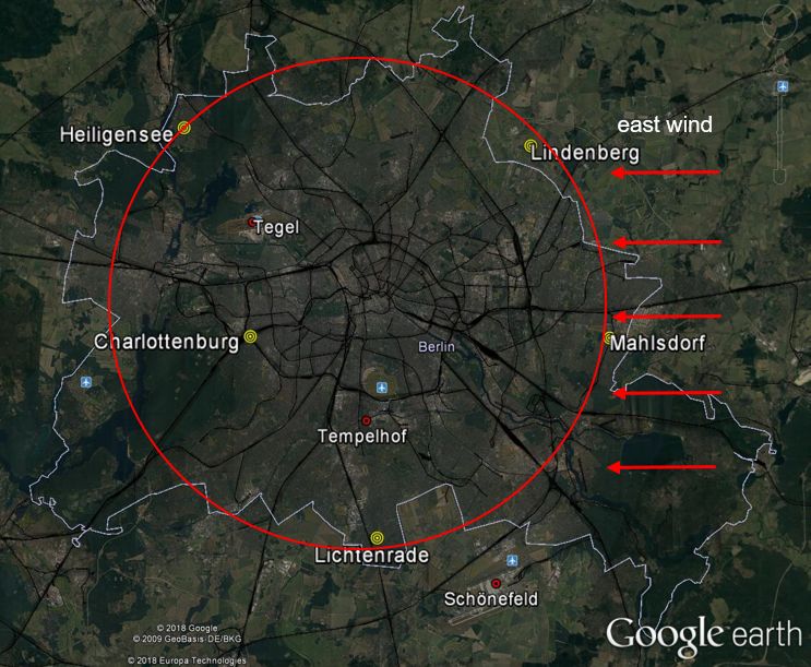
1    Introduction

     The share of greenhouse gas (GHG) emissions released from urban areas has continued to increase as a result of urbanization
20   (IEA, 2008; Kennedy et al., 2009; Parshall et al., 2010; IPCC, 2014). At present 55 % of the global population resides in urban
     areas (UNDESA, 2014), a number that is projected to rise to 68 % by 2050 (UNDESA, 2018). Meanwhile urban areas cover
     less than 3 % of the land surface worldwide (Wu et al., 2016), but consume over 66 % of the world’s energy (Fragkias et al.,
     2013), and generate more than 70 % of anthropogenic GHG emissions (Hopkins et al., 2016). Carbon dioxide (CO2 ) emissions
     from energy use in cities are estimated to comprise more than 75 % of the global energy-related CO2 , with a rise of 1.8 % per
25   year projected under business-as-usual scenarios between 2006 and 2030 (IEA, 2009). Methane (CH4 ) emissions from energy,
     waste, agriculture, and transportation in urban areas make up approximately 21 % of the global CH4 emissions (Marcotullio
     et al., 2013; Hopkins et al., 2016). As emission hotspots, urban areas therefore play a vital role in GHG mitigation. It is crucial
     to find appropriate methods for understanding and projecting the effects of GHG emissions on urban areas, and for formulating
     mitigation strategies.
30       There are two methods for the quantitative analysis of GHG emissions: the ‘bottom-up’ approach and the ‘top-down’ ap-
     proach (Pillai et al., 2011; Caulton et al., 2014; Newman et al., 2016). The ‘bottom-up’ approach calculates emissions based
     on activity data (i.e., a quantitative measure of the activity that can emit GHGs) and emission factors (Wang et al., 2009). This
     approach has some uncertainty, e.g., on the national fossil-fuel CO2 emission estimates, ranging from a few percent (e.g., 3 %-5
     % for the US) to a maximum of over 50 % for countries with less resources for data collection and poor statistical framework
35   (Andres et al., 2012). The considerable uncertainties are caused by the large variability of source-specific and country-specific
     emission factors and the incomplete understanding of emission processes (Montzka et al., 2011; Bergamaschi et al., 2015).
     These uncertainties grow larger at sub-national scales, when estimating the disaggregation of the national annual totals in
     space and time. The ‘top-down’ approach can not only provide estimated global fluxes, but also verify the consistency and as-
     sess the uncertainties of bottom-up emission inventories (Wunch et al., 2009; Montzka et al., 2011; Bergamaschi et al., 2018).
40   However, it is hard to quantify the statistical errors attached to both atmospheric observations and prior knowledge about the
     distribution of emissions and sinks (Cressot et al., 2014).
         McKain et al. (2012) suggested that column measurements can provide a promising route to improving the detection of CO2
     emitted from major source regions, possibly avoiding extensive surface measurements near such regions. Such measurements,
     i.e. measurements of concentration averaged over a column of air, are performed to help to disentangle the effects of atmo-
45   spheric mixing from the surface exchange (Wunch et al., 2011) and decrease the biases associated with estimates of carbon
     sources and sinks in atmospheric inversions (Olsen and Randerson, 2004). Compared to surface values, urban enhancements
     in columns are less sensitive to boundary-layer heights (Wunch et al., 2011; McKain et al., 2012; Kivi and Heikkinen, 2016)
     and column observations have the potential to mitigate mixing height errors in an atmospheric inversion system (Gerbig et al.,
     2008). Atmospheric GHG column measurements combined with inverse models are thus a promising method for analyzing
50   GHG emissions, and can be used to analyze their spatial and temporal variability (Ohyama et al., 2009; Pillai et al., 2011;
     Ostler et al., 2016; Kivi and Heikkinen, 2016).

                                                                     2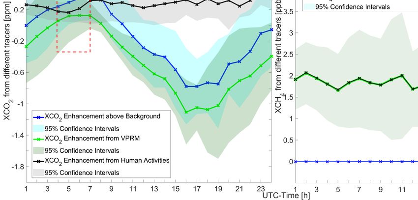
In order to focus the ‘top-down’ approach on concentration differences caused by local and regional emission sources, and
     in particular to quantify urban emissions, the differential column methodology (DCM) was proposed. It evaluates differences
     between column measurements at different sites. Chen et al. (2016) applied the DCM using compact Fourier Transform Spec-
55   trometers (FTS) EM27/SUN (Bruker Optik, Germany) and demonstrated the capability of differential column measurements
     for determining urban and local emissions in combination with column models. Citywide GHG column measurement cam-
     paigns have been carried out, e.g., in Boston (Chen et al., 2013), Indianapolis (Franklin et al., 2017), San Francisco, Berlin
     (Hase et al., 2015), and Munich (Chen et al., 2018). However, only a few studies have combined differential column mea-
     surements with high-resolution models. Toja-Silva et al. (2017) simulated the column data at upwind and downwind sites of
60   a gas-fired power plant in Munich using the Computational Fluid Dynamic model (CFD) and compared them with the col-
     umn measurements. Viatte et al. (2017) quantified CH4 emissions from the largest dairies in the southern California region,
     using four EM27/SUNs in combination with the Weather Research and Forecasting model (WRF) in large-eddy simulation
     mode. Vogel et al. (2019) deployed five EM27/SUN in the Paris metropolitan area and analyzed the data with the atmospheric
     transport model framework CHIMERE-CAMS.
65     This paper carries out a quantitative analysis of GHG for the Berlin area in combination with DCM. We utilize the mesoscale
     WRF model (Skamarock et al., 2008) coupled with GHG modules (WRF-GHG) (Beck et al., 2011) at a high resolution of 1
     km. The aim is to assess the precision of WRF-GHG and to provide insights on how to detect and understand sources of GHGs
     (CO2 and CH4 ) within urban areas. WRF is a numerical weather prediction system and can be used for both atmospheric
     research and operational forecasting, on a mesoscale range from tens of meters to thousands of kilometers, cf. e.g. (Chen
70   et al., 2011). To produce high-resolution regional simulations of atmospheric CH4 passive tracer transports, WRF was coupled
     with the Vegetation Photosynthesis and Respiration module (WRF-VPRM) (Ahmadov et al., 2007). WRF-VPRM has been
     widely employed in several studies, in which both the generally good agreement of the simulations with measurements and
     model biases have been assessed in detail (Ahmadov et al., 2009; Pillai et al., 2011, 2012; Kretschmer et al., 2012). Biogenic
     carbon fluxes given by the VPRM model tend to underestimate urban ecosystem carbon exchange, owing to the incomplete
75   understanding of urban vegetation, and to conditions related to urban heat islands and altered urban phenology (Hardiman
     et al., 2017). WRF-VPRM was later extended to WRF-GHG (Beck et al., 2011), which can simulate the regional passive tracer
     transport for GHGs (CH4 , CO2 and carbon monoxide (CO)). Relatively few studies using WRF-GHG have been published
     as yet. Pillai et al. (2016) utilized a Bayesian inversion approach based on WRF-GHG at a high spatial resolution of 10
     km for Berlin to obtain anthropogenic CO2 emissions, and to quantify the uncertainties in retrieved anthropogenic emissions
80   related to instruments (e.g. CarbonSat) and modelling errors. In the present paper, our focus is on a high-resolution (1 km)
     study of both CO2 and CH4 in Berlin, and assess the performance of WRF-GHG through comparing the simulated wind and
     concentration fields to observations from wind stations and ground-based solar-viewing spectrometers. Then DCM is tested
     as a proper approach for model analysis, which can cancel out the bias from initialization conditions and highlight regional
     emission tracers. The simulation workflow is also adapted to this purpose where needed. This study is the fundamental study
85   of the WRF-GHG mesoscale modeling framework in urban areas.

                                                                   3
The total annual CO2 emissions of Berlin (21.3 million tonnes in 2010) approximately correspond to those of Croatia, Jordan
      or the Dominican Republic (Reusswig and Lass, 2014). With its strong regulatory influence as a ‘state’ within Germany, and
      a strongly supportive policy, Berlin has already transformed itself into a climate-friendly city in which CO2 emissions have
      been reduced by a third compared with 1990 levels, aiming for carbon neutrality by 2050 (Homann, 2018). Berlin therefore
90    needs to assess and identify the emission sources accurately at the current stage, to provide solid scientific support for the
      selection of mitigation options. Additionally, Berlin is an ideal pilot case for developing and testing simulations because the
      city is relatively isolated from other large cities with high emissions, such that anthropogenic GHG anomalies around Berlin
      can confidently be attributed to the city itself.
          The major goals of our work in this context are: (1) to simulate high-resolution (1 km) CO2 and CH4 concentrations for Berlin
95    using WRF-GHG, attributing the changes in concentrations to different emission processes; (2) to compare the simulation
      outputs with the observations from a column measurement network in Berlin (Hase et al., 2015), assessing the precision of
      WRF-GHG; (3) to use DCM in the simulation analysis, testing the feasibly of this approach. The structure of this paper is
      as follows: The model with its domain and external data sources are described in Sect.2. A comparison analysis for wind
      fields and concentration fields is presented in Sect.3, and CO2 and CH4 concentrations related to different processes (e.g., the
100   anthropogenic component) are discussed. DCM for the comparison of concentration fields and the tracer analysis is presented
      and discussed in Sect.4. Section 5 provides the discussion and summary of this study.

      2    WRF-GHG Modeling System

      As mentioned in Sect.1, we use the WRF model Version 3.2 coupled with GHG modules to quantify the uptake and emission
      of atmospheric GHGs around Berlin at a high resolution of 1 km. WRF follows the fully compressible nonhydrostatic Euler
105   equations (Skamarock et al., 2005, 2008) and is based on the actual meteorological data in this case study. The meteorological
      initial conditions and lateral boundary conditions were taken from the Global Forecast System (GFS) model reanalysis in
      which in-situ measurements and satellite observations have been assimilated. Tracers in WRF-GHG are transported online in
      a passive way, i.e. without any chemical loss or production, when the tracer transport option is used (Ahmadov et al., 2007;
      Beck et al., 2011). As shown in Fig.1, three domains are set up here, whose dimensions are 70 × 50 horizontal grid points with
110   a spacing of 9 km for the coarsest domain (d01), 3 km for the middle domain (d02) and 1 km for the innermost domain (d03).
      WRF uses a terrain-following hydro-static pressure vertical coordinate (Skamarock et al., 2008). In our case, 26 vertical levels
      are defined from the surface up to 50 hPa, 14 of which are in the lowest 2 km of the atmosphere. The innermost domain, d03,
      envelops all five measurement sites (see Sect.3.1) to assess the simulation by comparing with the measured data. Berlin lies
      in the North European Plain on flat land (crossed by northward-flowing watercourses), which avoids the vertical interpolation
115   problems caused by topography differences (Fig.1). The Lambert conformal conic projection is selected as map projection.
      The simulated time span is from 18 UTC on 30th June to 00 UTC on 11th July in 2014. The description of the workflow for
      running WRF-GHG can be found in Appendix A.

                                                                      4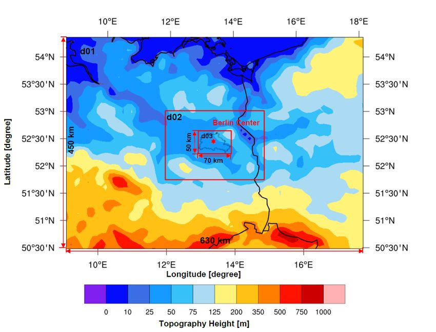
The meteorological fields are obtained from the Global Forecast System model (GFS) at a horizontal resolution of 0.5°
      with 64 vertical layers and a temporal resolution of 3 hours (as available via the NOAA-NCDC/NCEI, www.ncdc.noaa.gov).
120   The GFS uses hydrostatic equations for the prediction of atmospheric conditions, and its output includes large amounts of
      atmospheric and land-soil variables, wind fields, temperature, precipitation and soil moisture etc. The initial and lateral bound-
      ary conditions for our WRF-GHG concentration fields are implemented using Copernicus Atmosphere Monitoring Service
      (CAMS) data (Agusti-Panareda et al., 2017). CAMS provides the estimated mixing ratios of CO2 and CH4 with a spatial reso-
      lution of 0.8° on 137 vertical levels, with a temporal resolution of 6 hours (as available via https://atmosphere.copernicus.eu).
125     The simulation of CO2 and CH4 fluxes with different emission tracers in WRF-GHG is based on flux models and emission
      inventories which are either already implemented inside the model modules (‘online’ calculation) or constitute external datasets
      (‘offline’ calculation). The flux values from external emission inventories are converted into atmospheric concentrations and
      added to the corresponding tracer variables. In combination with the background concentration fields for CO2 and CH4 that
      refer to the CO2 and CH4 values without any sources and sinks in the targeted domain, the tracer contributions are summed up
130   to obtain the total concentrations, as

      CO2,total = CO2,bgd + CO2,VPRM + CO2,anthro + ∆CO2
                                                                                                                                     (1)
      CH4,total = CH4,bgd + CH4,anthro + CH4,soil + ∆CH4

      where CO2,total and CH4,total represent the total CO2 and CH4 , CO2,bgd and CH4,bgd are the background CO2 and CH4 , CO2,anthro
      and CH4,anthro stand for the changes in CO2 from the anthropogenic emissions, CO2,VPRM is the change in CO2 from the biogenic
      activities and CH4,soil is the change in CH4 from soil uptake, ∆CO2 and ∆CH4 are the tiny computational errors for CO2 and
135   CH4 described in detail in Appendix B. In the transport process, the relationship shown in Eq.1 holds for each vertical level.
        The biogenic CO2 emission is calculated online using VPRM (Mahadevan et al., 2008), in which the hourly Net Ecosys-
      tem Exchange (NEE) of CO2 reflects the biospheric fluxes between the terrestrial biosphere and the atmosphere, estimated
      by the sum of Gross Ecosystem Exchange (GEE) and Respiration. VPRM in WRF-GHG calculates biogenic fluxes initialized
      by vegetation indexes (land surface water index (LSWI), enhanced vegetation index (EVI), etc..) from the MODIS satellite
140   (as available via https://modis.gsfc.nasa.gov/). Combined with SYNMAP vegetation classification at a resolution of 1 km, the
      refectance data from the MODIS satellite at a 500-m spatial resolution and 8-day intervals is aggregated to the Lambert Con-
      formal Conic (LCC) projection within the WRF-VPRM preprocessor. Then, the data including these high-solution vegetation
      indexes at a resolution of 1 km are available on the model domains.
        We use the external dataset Emission Database for Global Atmospheric Research Version 4.1 (EDGAR V.4.1) for the anthro-
145   pogenic fluxes in our study. EDGAR V.4.1 provides annually varying global anthropogenic GHG emissions and air pollutants
      at a spatial resolution of 0.1° (Muntean et al., 2014; Janssens-Maenhout et al., 2015), whose source sectors include industrial
      processes, on-road and off-road sources in transport, large-scale biomass burning and other anthropogenic sources (Saikawa
      et al., 2017). Here we apply time factors for seasonal, weekly, daily and diurnal variations defined by the time profiles published
      on the EDGAR website (http://themasites.pbl.nl/tridion/en/themasites/edgar/documentation/content/Temporal-variation.html);
150   however, considerable uncertainties are to be expected in applying these time factors. This temporal variation set is derived

                                                                      5
based on western European data such that the representativity for other European countries and even other world regions may be
quite poor. The coarse emission fluxes used for the initialization of the anthropogenic tracer in WRF-GHG can cause problems
when locating emission points within the high-resolution model grid, and can weaken the impact from the real high emission
hot-spots in the fine domain of our study. The chemical sink for atmospheric CH4 (e.g., photo-chemistry in the stratosphere)
155 can be ignored in the model owing to its relatively long lifespan (9.5 ± 1.3 year, Holmes (2018)), the small-scale domains, and
the limited simulation period (10 days) in our case.
3 Model Analysis and Model-Measurement Comparison
3.1 Description of Measurement Sites
The measurement campaign used to compare with WRF-GHG in this paper was performed from 23rd June to 11th July 2014
160 in Berlin using five spectrometers (Hase et al., 2015). It allows us to both test the precision of WRF-GHG (Sect.3) and verify
differential column methodology (DCM) as our analytic methodology (Sect.4). In their measurement campaign, Hase et al.
(2015) used five portable Bruker EM27/SUN Fourier Transform Spectrometers (FTS) for atmospheric measurements based
on solar absorption spectroscopy. Five sampling stations around Berlin were set up, four of which (Mahlsdorf, Heiligensee,
Lindenberg and Lichtenrade) were roughly situated along a circle with a radius of 12 km around the center of Berlin. Another
165 sampling site was closer to the city center and located inside the Berlin motorway ring at Charlottenburg (Fig.6). Detailed
information on this measurement campaign is given in Hase et al. (2015) and Frey et al. (2015) provides additional details on
the calibration of the spectrometers, precision and instrument-to-instrument biases.
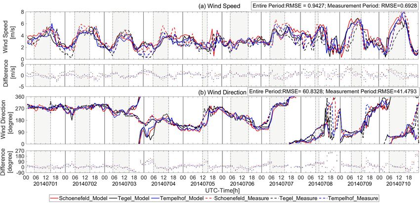
3.2 Comparison of Wind Fields at 10 meters
Winds have a strong impact on the vertical mixing of GHGs and a direct influence on their atmospheric transport patterns.
170 Hence, we firstly compare the wind speeds and wind directions obtained from WRF-GHG to the measurements, such that
deviations between the simulated and measured wind fields are assessed. The wind measurements are not exactly co-located
with the spectrometers mentioned in Sect.3.1, but rather are located at three sampling sites (Tegel, Schönefeld and Tempelhof,
respectively) and measure at a height of 10 meters above the ground. The simulated wind speed at 10 meters (ws10m ) and wind
direction at 10 meters (wd10m ) are calculated following the equations,
q
ws10m = u210m + v10m 2
175 v10m (2)
wd10m = arctan
u10m
where u10m and v10m are the components of the horizontal wind, towards the east and north respectively, which can be obtained
from WRF-GHG output files.
Figure.2 shows the comparisons of wind speeds (Fig.2(a)) and wind directions (Fig.2(b)) between simulations and observa-
tions at 10 meters from 1st July to 10th July and the model-measurement differences. EM27/SUN only operates in the daytime
6180 under enough sunlight (the detailed description of the instrument can be found in Gisi et al. (2012), Frey et al. (2015) and
Vogel et al. (2019)). The instrumental working periods are marked by gray shaded boxes in Fig.2. The measured (dashed lines)
and simulated (solid) wind speeds (Fig.2(a)) at 10 meters show similar trends and demonstrate relatively good agreement over
the 10-day time series with a root mean square error (RMSE) of 0.9247 m/s. Large uncertainties in wind speeds are found to
appear always with the lower wind speeds, mostly at night. In terms of wind directions at 10 meters, we observe that the sim-
185 ulated wind directions show similar but slightly underestimated fluctuations (Fig.2(b)), which result in a RMSE of 60.8328°.
Larger uncertainties in wind directions always exist during the low wind speed periods (Fig.2(a)&(b)). During the instrumental
working period (within the daytime), the simulations fit better with the measurements with relatively lower RMSEs 0.6928 m/s
for wind speeds and 41.4793° for wind directions. We find that the measured wind fields (both wind speeds and wind direc-
tions) have more fluctuations, compared to the simulations. This could be caused by real fast wind changes, which the model,
190 simulating a somewhat idealized environment, is not able to capture. To be specific, local turbulence given by urban canopy,
buildings etc. are not represented well in the model.
3.3 Comparison of pressure-weighted column-averaged concentrations
In the following, we use the measured concentration fields to compare with the simulated fields. An FTS EM27/SUN can
measure the column-integrated amount of a tracer through the atmospheric column with excellent precision, yielding the
195 column-averaged dry-air mole fractions (DMFs) of the target gases (Chen et al., 2016; Hedelius et al., 2016). The measured
DMFs of CO2 and CH4 are denoted by XCO2 and XCH4 . Hase et al. (2015) used constant a priori profile shapes in the retrievals
of measurements.
When comparing remote sensing observations to model data (or also datasets from different remote sensing instruments
to one another), limitations of the instruments in reconstructing the actual atmospheric state need to be taken into account.
200 In general, this requires the a-priori profile which was used for the retrieval and the averaging kernel matrix, which specifies
the loss of vertical resolution (fine vertical details of the actual trace gas profile cannot be resolved) and limited sensitivity
(e.g. Rodgers and Connor (2003)). In the case of EM27/SUN, the spectrometers used be the network offer only a low spectral
resolution of 0.5 cm−1 . Therefore, performing a simple least squares fit by scaling retrieval of the a-priori profile is generally
appropriate. In this case, there is no need to specify a full averaging kernel matrix, instead, the specification of a total column
205 sensitivity is sufficient. The total column sensitivity is a vector (being a function of altitude), which specifies to which degree
an excess partial column superimposed on the actual profile at a certain input altitude is reflected in the retrieved total column
amount. This sensitivity vector is a function of solar zenith angle (and ground pressure), mainly due to the fact that the
observed signal levels in different channels building the spectral scene used for the retrieval are shaped by a mixture of weaker
and stronger absorptions (if all spectral lines in the spectral scene would be optically thin and too narrow to be resolved by the
210 spectral measurement, the sensitivity would approach unity throughout).
In order to ensure measurement qualities and enough sample points for further concentration comparisons, we select five
measurement dates (1st , 3rd , 4th , 6th and 10th July) with relatively good measurement qualities (from fair ’++’ to very good
’++++’) based on Hase et al. (2015). The pressure-dependent column sensitivities for CO2 (Fig.3(b)) and CH4 (Fig.3(c))
7are derived from measurements performed in Lindenberg on 4th July (the best measurement-quality day). Details about the
215 measurements can be found in Hase et al. (2015) and Frey et al. (2015). The shape and values of the column sensitivities from
Karlsruhe closely resemble the results of Hedelius et al. (2016) in Pasadena. As depicted in Fig.3(a), the solar zenith angles
(SZAs) are almost identical for each day in our study (at each hour), rendering the shape of column sensitivities (at a specific
hour of the day) practically independent of the measurement date. The column sensitivities for 4th July (Fig.3(b,c)), are taken as
a basis for our smoothing process below. The a-priori CO2 and CH4 profiles are taken from the Whole Atmosphere Community
220 Climate model (WACCM) Version 6. A smoothed profile for a target gas G is then obtained as Eq.3 in (cf. Vogel et al., 2019),
Gs = K ∗ G + (I − K) ∗ Gp (3)
where G is the modelled profile from WRF-GHG for a target gas G, I is the identity matrix, K is a diagonal matrix containing
the averaging kernel, and Gp is the a-priori profile.
In order to compare the simulated smoothed concentration fields with the observations, the simulated smoothed pressure-
225 weighted column-averaged concentration for a target gas G (XG) is calculated as,
n
P (i) − P (i + 1) X
∆p(i) = → XG = ∆p(i) × Gs (i) (4)
Psf − Ptop i=1
Here, ∆pi is the proportional to the differences of the pressure values P (i) at the bottom and P (i + 1) at the top of the ith
vertical grid cell; Ptop and Psf represent the hydrostatic pressures at the top and at the surface of the model domain, and Gs (i)
stands for the simulated concentration of the target gas G at the ith vertical level.
230 In Figures.D1 and D2 of Appendix D, we compare the simulated XCO2 and XCH4 with and without smoothing. The
simulated concentrations are only slightly enlarged after smoothing, approximately 1-2 ppm for XCO2 and 2 ppb for XCH4 ,
while the variations are mostly not changed. Compare to the period with lower SZAs (at noon), the smoothed values in the
morning and afternoon with higher SZAs hold relatively larger enlargements.
Figure.4(a) shows the measured and modelled variations of XCO2 and XCH4 for these five days. Compared to the measure-
235 ments, the smoothed simulated pressure-weighted column-averaged concentrations for CO2 (XCO2 ) show quite similar trends
but with approx. 1-2 ppm bias, indicated by a RMSE of 1.2534 ppm. The simulated XCO2 are overestimated for 1st , 3rd and
4th July while on 6th and 10th July, the model is underestimated, which could attribute to the uncertainties from the coarse
anthropogenic surface emission fluxes, background concentrations from CAMS (Sembhi et al., 2015), and the ignorance of the
influence from the line of the sun sight.
240 Figure.4(b) shows the comparison of the pressure-weighted column-averaged concentrations for CH4 (XCH4 ) between ob-
servations and smoothed simulations on the five selected dates (1st , 3rd , 4th , 6th and 10th July). We find that there is an ap-
proximate offset of 50-60 ppb between observations and models (RMSE = 58.1082 ppb). The simulated XCH4 is around 1860
ppb while the measured value is around 1810 ppb which is comparable to the values (1790-1810 ppb) observed at two Total
Carbon Column Observing Network (TCCON) measurement sites in June and July 2014, Bremen in Germany (Notholt et al.,
245 2014) and Bialystok in Poland (Deutscher et al., 2014). This bias of the simulated XCH4 seems to be constant (around 2.7 %)
each day. Thus, we introduce an offset applied to all sites for each simulation date to compare the model and the measured
8data, effectively removing the bias, which we attribute to a too high background XCH4 . The daily offset is assumed to be the
difference between the simulated and measured daily mean XCH4 . After applying the daily offset, the measured XCH4 shows
a somewhat better agreement and a similar trend but with larger variability, compared to the simulation (RMSE = 3.1690 ppb).
250 The smaller variations from the simulation results can, e.g., be caused by the error from the spatial-temporal treatment of
emission maps, underestimated emissions from anthropogenic activities, the coarse wind data and/or the smoothing of actual
extreme values in the simulation.
A major offset in modelled CH4 concentration fields could potentially be attributed to the errors in the troposphere height
and a general offset from CAMS. In the CH4 vertical concentrations profile, we find that the typical sharp decrease is given
255 within the tropopause height. Tukiainen et al. (2016) also find the similar sharp decrease when using the air-cores to retrieve
the atmospheric CH4 profiles in Finland. During the simulation, the background concentration values of CAMS are directly
fitted to the WRF pressure axis, without the consideration of the actual tropopause height, thus this is unlikely to be the case.
An illustration of the vertical distribution for CH4 is provided in Appendix C. While the CO2 vertical distribution shows a
quite flat decrease with the increase of pressure and there is no need to consider the tropopause height during the grid treatment
260 in the vertical layer. Then in view of CAMS, the reports from Monitoring Atmospheric Composition and Climate (MACC)
described that CAMS held an increase of bias and RMSE (approx. 50 ppb) in each part of the world, compared to the Integrated
Carbon Observation System (ICOS) observations in 2017 (Basart et al., 2017). Galkowski et al. (2019) also mentioned one
CH4 offset (approx. 30 ppb within troposphere), when initializing the concentration fields using CAMS. Apart from these two
major potential reasons for the bias, the influence from the in-accurate simulated planetary boundary layers and the shape of the
265 constant a priori profile used for the retrievals both potentially contribute to the discrepancies for the concentration fields. Due
to the lack of fine measured vertical concentration profiles, it is not easy to quantify these errors and attribute these potential
reasons to this 2.7% error quantitatively. Thus, a DCM-based analysis is presented in Sect.4, aiming at eliminating the bias
from these relatively high initialization values for CH4 and making it easier to assess WRF-GHG results with respect to the
measurements.
270 3.4 Contributions of different sources and sinks to the total signal: Individual Emission Tracers
As described in Sect.2, the various flux models implemented in WRF-GHG are advected as separate tracers, making it possible
to distinguish the signals in concentration space for different source and sink categories for CO2 and CH4 (Beck et al., 2011).
Berlin is located in an area of low-lying, marshy woodlands with a mainly flat topography (Kindler et al., 2018). There is no
wetland in Berlin according to the MODIS Land Cover Map (Friedl et al., 2010). The land covered by forests, green and open
275 spaces (e.g., farmlands, parks, allotment gardens) accounts for 35 % of the total area in Berlin (SenStadtH, 2016). Addition-
ally, eleven power plants are currently being operated in Berlin, eight of which have a capacity over 100 MW (Fraunhofer-
Gesellschaft, 2018). In accordance with the geographical characteristics of the district and potential emission sources in Berlin,
we focus on understanding the major emissions caused by vegetation photosynthesis and respiration (XCO2,VPRM ) as well as
anthropogenic activities (XCO2,anthro ) for CO2 , and by soil uptake (XCH4,soil ) as well as human activities (XCH4,anthro ) for
280 CH4 .
9As an instructive example of an analysis involving these tracers, we look at the diurnal cycle of contributions from the
different tracers mentioned above in Charlottenburg (Fig.5). The mean values, averaged over 9 days (from 2nd to 10th July)
as well as a 95 % confidential interval calculated in the averaging process are shown in Fig.5. Figure.5(a) clearly shows a
decline during the day and a rise at night in the XCO2 enhancement over the background (blue: XCO2,total - XCO2,bgd ),
285 with a maximum decrease over the course of the day of around 2 ppm. The XCO2 enhancement over the background reaches
its daily peak during morning rush hour (07 UTC). The morning peak corresponds to XCO2 changes from human activities,
depicted by the black line from 04 UTC to 07 UTC (marked by a red square in Fig.5(a)). Before the evening rush hour (16
UTC), XCO2 over the background then decreases, owning to biogenic uptake. Beginning in the evening, values increase again.
The fluctuation in the evening (17 UTC – 19 UTC) are dominated by XCO2 enhancements from human activities while
290 the substantial rise from 19 UTC onward is generated by the VPRM tracer, specifically the accumulation of the vegetation
respiration in the evening.
XCO2 is weaker compared to the strong biogenic uptake. To further highlight the role of anthropogenic activities in XCO2
changes within the urban area, DCM is applied in Sect.4. More specifically, we will use downwind-minus-upwind column
differences of CO2 (∆XCO2 ) to describe the XCO2 enhancement over an upwind site, as the difference between the downwind
295 and upwind sites can be attributed to urban emissions.
Turning to XCH4 in Fig.5(b), we plot the variations of the mean hourly contributions from the anthropogenic (black line:
XCH4,anthro ) and soil uptake tracer (blue: XCH4,soil ) in Charlottenburg. The contributions by anthropogenic activities fluctuate
slightly around 2 ppb in the morning and at noon; then a peak occurs at the start of the evening rush hour (16 UTC). After
18 UTC, values clearly decrease, reaching approximately 2 ppb. From 21 UTC XCH4 stabilizes, exhibiting only moderate
300 fluctuations. The XCH4 enhancement above the background (green: XCH4,total - XCH4,bgd ) depends largely on the XCH4
contributions by human activities. The changes in concentrations caused by the soil uptake tracer (blue), whose values fluctuate
between 0.001 ppb and 0.01 ppb, have almost no influence on the variation of the XCH4 enhancement over background in the
urban area.
4 Model Analysis using Differential Column Methodology
305 4.1 Comparison of differential column concentrations
The differential column methodology (DCM) can be employed to detect and estimate local emission sources within an area,
based on calculated concentration differences between downwind and upwind sites (Chen et al., 2016). The difference (∆XG)
of a specific gas G in column-averaged DMFs across the downwind and upwind sites is defined as,
∆XG = XGdownwind − XGupwind (5)
310 where XGdownwind and XGupwind represent the column-average DMFs at the downwind and upwind sites.
10In this study, DCM is applied to measurements and models in the spirit of a post-processing analysis. This approach is not
only useful to cancel out the bias of the simulated XCH4 (see Sect.3.3), but also to assess the role of anthropogenic activities
in XCO2 changes more appropriately.
A necessary prerequisite for DCM is distinguishing the upwind and downwind sites among all five sampling sites. Wind
315 direction thus plays a pivotal role in the calculation of the downwind-minus-upwind column differences. In this study, the
hourly simulated vertical-averaged wind directions are assumed as a standard to classify the sites into downwind and upwind
sites. The tracer transport calculations in the first few hours are not stable in WRF-GHG. Thus, we select 3rd , 4th , 6th and 10th
as our targeted dates.
Table.1 shows the daily average wind directions with standard derivations and the details on the downwind and upwind
320 sites for these four target dates. West wind is the prevailing wind direction on 3rd . That is to say, Mahlsdorf and Lindenberg
are downwind sites, and the upwind sites corresponding to these are Charlottenburg and Heiligensee. While the wind on 10th
July is northeasterly and the combination of downwind and upwind sites are selected to be opposite of the ones on 3rd July.
The prevailing wind on 4th and 6th are easterly. The upwind site is Lichtenrade, and the corresponding downwind sites are
Heiligensee and Lindenberg. Based on the selection of downwind and upwind sites shown in Table.1 and Eq.5, differential
325 column concentrations (∆XCH4 ) are, therefore, respectively, calculated as:
West Wind (3rd July) : ∆XCH4 = (XCH4Mahlsdorf + XCH4Lindenberg )/2 − (XCH4Charlottenburg + XCH4Lichtenrade )/2 (6)
North Wind (4th and 6th July) : ∆XCH4 = (XCH4Heiligensee + XCH4Lindenberg )/2 − XCH4Lichtenrade (7)
Northeast Wind (10th July) : ∆XCH4 = (XCH4Charlottenburg + XCH4Lichtenrade )/2 − (XCH4Mahlsdorf + XCH4Lindenberg )/2 (8)
Figure.7 depicts the variations of the wind fields (wind speeds and wind directions) and ∆XCH4 (corresponding to Eq.6, 7
330 and 8) on 3rd , 4th , 6th and 10th July. As depicted in the left column of Fig.7, the hourly vertical-mean simulated wind speeds
and directions at downwind and upwind sites are homogeneous. Thus, it is reasonable to use the daily mean wind directions
as the standard for the selection of downwind and upwind sites. The general trends in the simulated ∆XCH4 values, shown
in the right column of Fig.7, seem to be roughly reproduced by the observations but slightly overestimated, with a RMSE of
1.3895 ppb.
335 Yet, DCM as presented here has potential to highlight the role of anthropogenic activities, which we demonstrate applying it
to CO2 tracers in the simulation. Thus, the analysis on anthropogenic and biogenic tracers for CO2 will be specially prominent
here. As described above, we continue to take 3rd , 4th , 6th and 10th July as examples (see the left column of Fig. 8).
With the left column of Fig.8, the variations of ∆XCO2 (corresponding to Eq.6, 7 and 8) on 3rd , 4th , 6th and 10th are shown.
In contrast to XCO2 values (Sect.3.4, Fig.5(a)), the simulated ∆XCO2 (Fig.8, left column, blue lines) is not so much influenced
340 by the XCO2 changes from the VPRM tracer (Fig.8, left column, green), but more closely follows the XCO2 changes from
anthropogenic activities (Fig.8, left column, red). With DCM, the role of human activities in XCO2 changes is highlighted and
the strong effect from the biogenic component is canceled out. The ∆XCO2 measurements (Fig.8, left column, black) show
similar trends as the simulation with a RMSE of 0.2973 ppm.
11To further understand the differences of ∆XCO2 and ∆XCH4 between measurements and simulations (see Fig.7, right
345 column and Fig.8, left column), the comparisons of hourly mean ∆XCO2 and ∆XCH4 values for these four targeted dates
are illustrated in the right column of Fig.8. Due to the restriction of measured wind information, we illustrate the differences
of simulated and measured wind directions at 10 meters (i.e. Fig.2(b)) with respect to the hourly mean ∆XCO2 and ∆XCH4 .
We find that the real hourly mean ∆XCO2 and ∆XCH4 values are generally higher than the simulated values. Extreme points
are colored red and blue in the right column of Fig.8, standing for large differences between measured and simulated wind
350 directions at 10 meters. We see that a large difference of wind directions is a necessary but insufficient condition for the bias
of ∆XCO2 and ∆XCH4 between measurements and simulations. In future studies, this is suggested to be verified further.
We conclude that DCM, as applied in this plot, reduces the model bias caused by the simulation initialization, but introduces
unpleasant effects which may be attributed to errors in the assumed or simulated wind directions.
4.2 Comparison between differential column concentrations and modeling results after the elimination of wind
355 influence
As described in Sect.4.1, the wind direction impacts the distinction between downwind and upwind sites for DCM. Devising
meaningful and accurate recipes for determining the wind directions is not easy, sometimes resulting in mixed-quality results
(of Sect.4.1). Our simulated output provides the hourly wind and concentration fields. The instruments measure the concentra-
tion value every minute (Hase et al., 2015) We simply assume the wind direction to be a constant value within one hour (the
360 hourly vertical-averaged values) in our calculation, also when it comes to selecting up- and downwind sites. This may create
inaccuracies in the calculation of the measured ∆XCH4 .
In this section, we test replacing the upwind values in DCM by an all-site mean to provide a potential solution for the
elimination of such problems while still applying the DCM. The mean of the column-averaged DMFs over all sampling sites
(XGspecific site ) is assumed to be the background concentration within the entire urban region, replacing the XCH4 at the upwind
365 site. The differences between the specific site and the mean of all the sites for each gas G (∆XGspecific site ) is then evaluated,
i.e.
∆XGspecific site = XGspecific site − XGall sites (9)
where XGspecific site is the column-averaged DMF at the respective sampling site.
We now test this form of DCM for the same four targeted dates (3rd , 4th , 6th and 10th July). The distance between any two
370 sampling sites is around 25 km. The general trends of the simulated (Fig.9, blue lines) and measured (Fig.9, black) ∆XCH4
appear to be more similar with a RMSE of 0.6698 ppb, compared to the comparison of ∆XCH4 in the right column of Fig.7
(RMSE=1.3895 ppb). The measurement-model bias can be caused by underestimated emissions from anthropogenic activities,
the smoothing of actual extreme values in the simulation and the ignorance of the line of the sun sight for the simulation. The
variations of the XCH4 at the five different sampling sites on the same day are similar (Fig.9), but the measurements show
375 more extreme values (e.g., 4th July), compared to the simulations. A further analysis in a future study is suggested to provide
deeper insight on site-specific transport characteristics.
12As a final point in our analysis, we focus on simulated ∆XCO2 values for these four target dates (Fig.10). The ∆XCO2
(blue line) on 3rd , 4th , 6th and 10th July in five sampling sites are mainly dominated by the XCO2 changes caused by the
anthropogenic tracer (red), instead of the VPRM tracer (green). Compared to the left column of Figure.8, the red line and
380 blue line in Fig.10 show a stronger similarity in their trends. With this form of DCM (compared to the original form Eq.5
in Sect.4.1), anthropogenic activities can be clearly shown to influence XCO2 within urban areas. Meanwhile, the ∆XCO2
measurements (black) fit better with the simulation with a RMSE of 0.2333 ppm, compared to the comparisons of ∆XCO2
depicted in the left column of Fig.7 (RMSE=0.2973 ppm).
5 Discussion and conclusion
385 We used WRF-GHG to quantitatively simulate the uptake, emission and transport of CO2 and CH4 for Berlin with a high
resolution of 1 km. The simulated wind and concentration fields were compared with observations from 2014. Then, differential
column methodology (DCM) was utilized as a post-processing method for the XCH4 comparison and the XCO2 tracer analysis.
The measured and simulated wind fields at 10 meters mostly demonstrate good agreement but with slight errors in the wind
directions. The simulated pressure vertical profile and the averaging kernel from the solar-viewing spectrometer (EM27/SUN)
390 are used to obtain the smoothed pressure-weighted average concentration for further comparisons. The simulated XCO2 con-
centrations actually reproduce the observations well, but with approx. 1-2 ppm bias which can attribute to the coarse emission
inventory, background concentrations from CAMS and the ignorance of the line of the sun sight for the simulation. Compared
with the measured XCH4 , some deviations can clearly be noted in the the simulated XCH4 , caused by the relatively high
initialization of background concentration fields and the errors in the tropopause height potentially. We discussed the diurnal
395 variation of concentration components corresponding to the major emission tracers for both CO2 and CH4 . The biogenic com-
ponent plays a pivotal role in the variations of XCO2 . The impact from anthropogenic emission sources is somewhat weak
compared to this, while the XCH4 enhancement is dominated by human activities.
We then concentrated on using DCM for focusing our analysis on relevant CO2 and CH4 contributions from the urban area.
DCM highlights that the enhancement of XCO2 over background within the inner Berlin urban area is mostly caused by anthro-
400 pogenic activities. In DCM, wind direction plays a vital role to define the upwind and downwind sites, which directly influence
the calculation of differential column concentrations. In the CO2 tracer analysis, it turns out that ∆XCO2 , the difference with
respect to a mean value instead of a specific upwind site, exhibits a more visible and clearer trend, which proves that the
CO2 enhancement is dominated by anthropogenic activities within the urban area. We conclude that DCM, when applied with
care, helps to highlight the relevant emission sources. Similarly, for XCH4 , DCM eliminates the bias of the simulated values.
405 Furthermore, when ∆XCH4 values suffer from inconsistent wind directions, we consider ∆XCH4 to be a useful quantity for
analysis.
An analysis of XCO2 in the Paris hot-spot region was carried out by Vogel et al. (2019). Some of their results can be compared
to the conclusions we drew in this paper. In Vogel et al. (2019), the modelled XCO2 was calculated based on the chemistry
transport model CHIMERE (2 km) and flux framework CAMS (15 km), with hourly anthropogenic emissions from the IER
13410 and EDGAR emission inventories, and the natural fluxes prescribed by the C-Tessel model (Sect.2 in Vogel et al. (2019)).
When comparing results from our simulation, the diurnal variation in the XCO2 enhancement over background (Sect.3.4 and
Fig.4(a) of our paper) is comparable to the findings of Vogel et al. (2019). For the analysis on the comparison of ∆XCH4
between simulations and measurements in Sect.4.1, we found that negative column concentration differences between down-
and upwind sites appear for some periods, owing to the variation of wind directions that causes the conversion of up- and
415 downwind sites, which was also mentioned for the ∆XCO2 analysis in Vogel et al. (2019). Based on the CHIMERE-CAMS
modelling framework, they showed that the strong decrease in XCO2 during daytime can be linked to net ecosystem exchange,
while a significant enhancement compared to the background is caused by XCO2 from fossil fuel emissions, but this is often
compensated by net ecosystem exchange. We utilized DCM to bring out the role of anthropogenic activities within urban areas
(see the XCO2 tracer analysis in Sect.4 of our paper).
420 We conclude that WRF-GHG is a suitable model for precise GHG transport analysis in urban areas, especially when com-
bined with DCM. DCM is not only useful for the direct evaluation of measurements, but also helps us to understand the results
of tracer transport models, canceling out the bias caused, e.g., by initialization conditions, and highlighting regional emission
sources. This case is a fundamental study for the WRF-GHG mesoscale modelling framework which is being built to combined
with the first worldwide permanent fully-automated column network for GHGs and NOx in Munich.
425 In future work, we suggest running WRF-GHG for more urban areas, such that, e.g., different transport, more emission
tracers, topography, emission scenarios and the quantification of model errors can be studied. The influence from the line
of the sun sight should be taken into account and the relative sensitivity analysis is suggested. The WRF-GHG mesoscale
simulation framework may also be combined with microscale atmospheric transport models to simulate crucial details of
emission sources and transport patterns precisely, with the aim of tracing urban GHG emissions. A further promising direction
430 for future studies may be the application of DCM and model-based analysis to satellite measurements, to assess gradients
across column concentrations with a dense spatial sampling.
Author contributions.
Xinxu Zhao performed the simulations, with the support and guidance of Julia Marshall, Christoph Gerbig, Jia Chen and
Stephan Hachinger. Julia Marshall provided the CAMS fields for the initialization. Jia Chen supplied anthropogenic emission
435 source and Christoph Gerbig offered the VPRM used for the simulations. Matthias Frey and Frank Hase provided the measure-
ment data for Berlin in 2014 and fruitful discussions related to the measurements. Stephan Hachinger provided the guidance
related to the running of the simulations in the Linux Cluster. Xinxu Zhao, Jia Chen and Stephan Hachinger designed the
computational framework. Xinxu Zhao and Jia Chen performed the analysis of the results. Xinxu Zhao wrote the manuscript
with input from all authors. All authors provided critical feedback and helped shape the research, analysis and manuscript.
440 Data availability.
14The simulation data that support the findings of this study are available on request from the corresponding author. The
measurement data are available at doi:10.5194/amt-8-3059-2015 (Hase et al., 2015).
Competing interests.
The authors declare that they have no conflict of interest.
445 Acknowledgements. We thank the personal contribution from Dr. Michal Galkowski from Max Plank Institute for Biogeochemistry for the
biogenic-related CH4 flux estimates. The priori concentration profiles from the whole Atmoshpere Community Climate Model (WACCM)
were provided by J.Hannigan (NCAR). Jia Chen is partly supported by Technische Universität München – Institute for Advanced Study,
funded by the German Excellence Initiative and the European Union Seventh Framework Programme under grant agreement no. 291763.
The simulations presented in this work have been run on the Linux Cluster (CooLMUC-2) of the Leibniz Supercomputing Centre (LRZ,
450 Garching).
15Figure 1. The topography map for the three domains in our study. The domain d03 is centered over Berlin, at 13.383°N, 52.517°E, marked
with a red star. The boundary of Berlin from GADM (available at https://gadm.org/) is depicted in the innermost domain.
16Figure 2. Variation and differences between simulated and measured wind fields for (a) wind speeds and (b) wind directions from 1st to
10th July 2014 at the three measurement sites, Schönefeld (red lines), Tegel (black) and Tempelhof (blue) in Berlin. The solid lines represent
the simulated wind fields provided by WRF-GHG and the dashed lines depict the measured wind fields. The differences in (a)&(b) are
simulations minus measurements. FTS measurement time periods on each date are marked by gray shaded areas.
(a) Solar Zenith Angels (SZA) (b) 20140704 - CO2 (c) 20140704 - CH4
110 0
SZA in 20140701 06:00 SZA 64.492°
SZA in 20140703 100
100 SZA in 20140704 07:00 SZA 55.593°
SZA in 20140706
SZA in 201407010 200 08:00 SZA 46.743°
90
09:00 SZA 38.754°
300
80 10:00 SZA 32.612°
Pressure [hPa]
400
SZA [degree]
11:00 SZA 29.718°
70
500 12:00 SZA 31.078°
60 13:00 SZA 36.184°
600
14:00 SZA 43.630°
50
700 15:00 SZA 52.250°
40 16:00 SZA 61.316°
800
17:00 SZA 70.357°
30 900
18:00 SZA 79.001°
1000
20
1 4 7 10 13 16 19 22 24 0 0.5 1 1.5 0 0.5 1 1.5
UTC-Time [h] Column Sensitivities
Figure 3. (a) Daily variations of solar zenith angle (SZA) for five simulation dates (1st , 3rd , 4th , 6th and 10th July) and the vertical distributions
of column sensitivities for (b) CO2 and (c) CH4 on 4th July. (b) & (c): the solid lines represent our derived column sensitivities for EM27/SUN
under different SZAs, and the circles stand for the values on model pressure levels.
17(a) XCO2 RMSE=1.2534
398
XCO2 [ppm]
396
394
392
390
(b) XCH4 RMSE=58.1082
1880
XCH4[ppb]
1860
(c) Modeled XCH4 - offset RMSE=3.1690
1830
1820
1810
1800
8 12 16 8 12 16 8 12 16 8 12 16 8 12 16
20140701 Q='++' 20140703 Q='+++' 20140704 Q='++++' 20140706 Q='++' 20140710 Q='++'
UTC-time[h]
Charl_Model Measure Heili_Model Measure Lind_Model Measure Licht_Model Measure Mahls_Model Measure
Figure 4. Variations of the measured and smoothed simulated (a) XCO2 and (b) XCH4 on 1st , 3rd , 4th , 6th and 10th July 2014, for five sampling
sites in Berlin: Charlottenburg (Charl: black markers), Heiligensee (Heili: purple), Lichtenrade (Licht: green), Lindenberg (Lind: blue) and
Mahlsdorf (Mahls: red). The solid circles in (a) and (b) stand for the simulated values provided by WRF-GHG and the dashed lines represent
the measured concentrations. The solid circles represent the simulated XCH4 after the subtraction of the daily offset in (c).
Figure 5. The diurnal variations of the simulated changes in concentrations caused by different emission tracers in Charlottenburg in Berlin
from 2014, averaged over a period of nine days (from 2nd to 10th July 2014). The colored lines represent the concentration changes and the
mean enhancement over background. (a): the mean hourly XCO2,VPRM (green line) and XCO2,anthro (black); (b): the mean hourly XCH4,anthro
(black) and XCH4,soil (blue). The red box in (a) marks the morning peak of the XCO2 enhancement over the background, as described in
Sect.3.4.
18Figure 6. Detailed locations of the five sampling sites.The five red stars stand for the five sampling sites, four of which (Mahlsdorf, Heili-
gensee, Lindenberg and Lichtenrade) were roughly situated along a circle with a radius of 12 km around the center of Berlin, marked as
the black circle. The innermost domain of our WRF-GHG model contains all five measurement sites. The three wind measurement sites are
marked by red circles. Map provided by Google Earth.
1920140703 20140703
12
4
2
10 0
-2
8 -4
20140704 20140704
10 4
Wind Direction [Degrees]
9 2
XCH4 [ppb]
Wind Speed [m/s]
0
8 -2
-4
20140706 20140706
7
4
2
6 0
-2
5 -4
20140710 20140710
12
4
11 2
0
10
-2
9 -4
7 9 11 13 15 UTC-Time [h] 7 9 11 13 15
Wind Speed_downwind Wind Speed_upwind Simulated XCH4 Measured XCH4 RMSE=1.3895
Wind Direction_downwind Wind Direction_upwind
Figure 7. Modeled wind fields for downwind (blue lines) and upwind (red) sites (left column), and downwind-minus-upwind differential
evaluation for measured (blue) and simulated (black) XCH4 (right column) on 3rd , 4th , 6th and 10th July 2014. Based on the selection of
downwind and upwind sites in Table.1, ∆XCH4 is calculated using Eq.6, 7 and 8, depicted by blue lines for measurements and black lines
for simulations. The black error bars in the right column are the standard derivations of the minute values of the hourly mean.
20140703 2
0.5
Simulated XCO2
XCO2 [ppm]
RMSE=0.2973
0 Simulated XCO2,anthro
1
Simulated XCO2,VPRM
-0.5
Measured XCO2
-1 0
Difference of Simulated and Measured
20140704
Measured
40
Wind Directions at 10m [degree]
0
-1
20
-0.5
-2 0
-1 -2 -1 0 1 2
20140706 Simulated XCO2 [ppm]
0 2 -20
XCH4 [ppb]
-0.5 -40
1
-60
-1 0
20140710
Measured
-1
0.5
-1
0
-0.5
-2
-1 -2 -1 0 1 2
UTC-Time [h] Simulated XCH4 [ppb]
Figure 8. Measured (black lines) and simulated (blue) ∆XCO2 on 3rd , 4th , 6th and 10th July 2014, and Comparison of hourly mean ∆XCO2
and ∆XCH4 for these four days. The ∆XCO2 , calculated using Eq.6, 7 and 8, are depicted by blue lines in the right column. The red and
green lines show the variation of the differences between downwind and upwind sites in XCO2 changes from anthropogenic and biogenic
activities, respectively. The points color in right column are coded by the difference of the simulated and measured wind directions at 10
meters. The black error bars in the left column are the standard derivations of the minute values of the hourly mean.
204
(a) Char 2
0
-2
4
XCH4 Changes from different tracers [ppb]
(b) Heili 2
0
-2
3
(c) Lind 1
-1
-3
4
(d) Licht
2
0
-2
2
(e) Mahls
0
RMSE=0.6697
-2
06 12 18 06 12 18 06 12 18 06 12 18
20140703 20140704 20140706 20140710
UTC-Time [h]
Figure 9. Modelled (blue lines) and observed (black) site XCH4 vs. site-mean XCH4 data for five sampling sites: Charlottenburg (Char: 1st
row), Heiligensee (Heili: 2nd row), Lindenberg (Lind: 3rd row), Lichtenrade (Licht: 4th row) and Mahlsdorf (Mahls: 5th row). The black error
bars in each subplot are the standard derivations of the minute values of the hourly mean.
1
(a) Charl 0
-1
XCO2 Changes from different Tracers [ppm]
0.5
(b) Heili 0
-0.5
1
0.5
(c) Lind
0
-0.5
0.5
(d) Licht 0
-0.5
0.4
(e) Mahls
RMSE=0.2333
0.2
-0.8
06 12 18 06 12 18 06 12 18 06 12 18
20140703 20140704 20140706 20140710
Figure 10. ∆XCO2 (blue lines for simulations and black for measurements) for five sampling sites (i.e. the difference between XCO2 at the
site and the mean XCO2 of five sampling sites): Charlottenburg (Char: 1st row), Heiligensee (Heili: 2nd row), Lindenberg (Lind: 3rd row),
Lichtenrade (Licht: 4th row) and Mahlsdorf (Mahls: 5th row). We furthermore show the differences in the simulated XCO2 changes from
biogenic (green) and anthropogenic (red) activities. The black error bars in each subplot are the standard derivations of the minute values of
the hourly mean.
21You can also read