A Multivariate Data Mining Approach to Predict Match Outcome in One-Day International Cricket - PAF-KIET
←
→
Page content transcription
If your browser does not render page correctly, please read the page content below
A Multivariate Data Mining Approach to
  Predict Match Outcome in One-Day
         International Cricket

   Author:                                              Supervisor:
   Waqar Ahmed                               Dr. Khurram Nazir

             A thesis submitted in fulfillment of the
                 requirements for the degree of

                     Master of Science

     Graduate School of Science and Engineering
  PAF - Karachi Institute of Economics and Technology

                        August 2015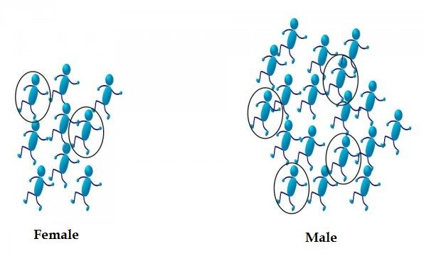
I would like to dedicate this thesis to my loving parents . . .
Declaration

I hereby declare that this document contains no material which has been accepted for the
award to the candidate of any other degree or diploma, except where due reference is made to
the work of others. This thesis is my own work and contains nothing which is the outcome of
work done in collaboration with others, except as specified in the text and Acknowledgements.

                                                                             Waqar Ahmed
                                                                               August 2015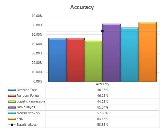
Acknowledgments

Firstly, I am more than grateful to almighty ALLAH made me able to carry out this research
for the degree of Master of Science at PAF KIET.
   Secondly, it is my great pleasure to acknowledge that this research has been done under
the supervision of Dr. Khurram Nazir, Assistant Professor PAF KIET. I am very thankful to
him for his sincere guidance, valuable comments, support and encouragement. Surely, he is
the most courteous and gracious person, I have ever met. In particular, his knowledge, humor,
insight, persistence and tolerance that have made this dissertation possible. I am extremely
grateful to Dr. Tariq Mahmood too, who suggested me this topic and persistently guided me
in carrying out the research.
   Finally, I would like to thank to my two friend Maarij Raheem and Mohammad Danish
for their valuable support and praiseworthy effort in data collection. This thesis would not
have been possible without these incredible fellows. Especially, I am grateful to my parents
and siblings for their unmatchable love, support, encouragement and prayers.
Abstract

Analyzing time oriented data and forecasting are among the most important problems that
analysts face in data mining. In this dissertation, a prediction model for new time series
forecasting problem i.e. prediction of One-Day International (ODI) cricket match outcome
for Pakistan team against all international oppositions has been presented.
   Enormous effort has been putted in collection of raw data and preprocessing for the range
of variables that could define the outcome of an ODI cricket match. Decisive attributes
were identified through exhaustive search, especially an attribute "Consecutive wins before
current match" was introduced which has not been used in the literature earlier. Several
unique approaches adopted for dataset formation and classification model learning that allow
one to predict the match outcome with 80% accuracy which is far greater than the work
previously shown in literature.
   Various machine-learning algorithms applied on different sizes of training and testing data
sets. It has been found that k-Nearest Neighbors (kNN) has outperformed 5 other renowned
classification algorithms (e.g. Decision Tree, Random Forest, Naive Bayes, Artificial Neural
Network and Logistic Regression) that has not been presented in literature yet as far as
prediction of ODI match outcome is concerned. The prediction model can be used to
benefit Pakistan Cricket Board (PCB) by assessing the merits of certain strategies of play.
Furthermore, cricket analysts, media and gamblers can also use the model for pre-match
analysis.
Table of contents

List of figures                                                                               xv

List of tables                                                                               xvii

1   Introduction                                                                               1
    1.1   Aims and Objectives . . . . . . . . . . . . . . . . . . . . . . . . . . . . .        2
    1.2   The Game of cricket . . . . . . . . . . . . . . . . . . . . . . . . . . . . .        3
    1.3   Motivation . . . . . . . . . . . . . . . . . . . . . . . . . . . . . . . . . . .     4
    1.4   Research Question . . . . . . . . . . . . . . . . . . . . . . . . . . . . . .        5
    1.5   Thesis Structure and Contribution . . . . . . . . . . . . . . . . . . . . . .        5

2   Literature Review                                                                          7
    2.1   Related Work . . . . . . . . . . . . . . . . . . . . . . . . . . . . . . . . .       7

3   Methodology                                                                               11
    3.1   Background . . . . . . . . . . . . . . . . . . . . . . . . . . . . . . . . . .      11
    3.2   Target Team . . . . . . . . . . . . . . . . . . . . . . . . . . . . . . . . . .     12
    3.3   Winning Pattern of Pakistan against each Team . . . . . . . . . . . . . . .         14
    3.4   Dataset . . . . . . . . . . . . . . . . . . . . . . . . . . . . . . . . . . . .     19
          3.4.1    Data Collection . . . . . . . . . . . . . . . . . . . . . . . . . . . .    19
    3.5   Preprocessing . . . . . . . . . . . . . . . . . . . . . . . . . . . . . . . . .     20
          3.5.1    Home advantage . . . . . . . . . . . . . . . . . . . . . . . . . . .       21
          3.5.2    Pitch Report . . . . . . . . . . . . . . . . . . . . . . . . . . . . .     22
xii
3.5.3 Weather Report . . . . . . . . . . . . . . . . . . . . . . . . . . . . 22
3.5.4 ODI# . . . . . . . . . . . . . . . . . . . . . . . . . . . . . . . . . 28
3.5.5 Date . . . . . . . . . . . . . . . . . . . . . . . . . . . . . . . . . . 28
3.5.6 Season . . . . . . . . . . . . . . . . . . . . . . . . . . . . . . . . 29
3.5.7 Opposition . . . . . . . . . . . . . . . . . . . . . . . . . . . . . . 30
3.5.8 Country . . . . . . . . . . . . . . . . . . . . . . . . . . . . . . . . 30
3.5.9 Ground . . . . . . . . . . . . . . . . . . . . . . . . . . . . . . . . 30
3.5.10 Day/Night . . . . . . . . . . . . . . . . . . . . . . . . . . . . . . . 30
3.5.11 Batting First . . . . . . . . . . . . . . . . . . . . . . . . . . . . . 30
3.5.12 Consecutive Wins before Current Match . . . . . . . . . . . . . . . 31
3.5.13 Pak Win . . . . . . . . . . . . . . . . . . . . . . . . . . . . . . . . 31
3.6 Classification Methods . . . . . . . . . . . . . . . . . . . . . . . . . . . . 31
3.6.1 k-Nearest Neighbors . . . . . . . . . . . . . . . . . . . . . . . . . 31
3.6.2 Artificial Neural Network . . . . . . . . . . . . . . . . . . . . . . 32
3.6.3 Decision Trees . . . . . . . . . . . . . . . . . . . . . . . . . . . . 33
3.6.4 Random Forest . . . . . . . . . . . . . . . . . . . . . . . . . . . . 33
3.6.5 Logistic regression . . . . . . . . . . . . . . . . . . . . . . . . . . 34
3.6.6 Naïve Bayes . . . . . . . . . . . . . . . . . . . . . . . . . . . . . 34
4 Experimental Details and Results 37
4.1 Attribute Selection . . . . . . . . . . . . . . . . . . . . . . . . . . . . . . 37
4.2 Sampling Technique . . . . . . . . . . . . . . . . . . . . . . . . . . . . . 41
4.3 Experimental Setup . . . . . . . . . . . . . . . . . . . . . . . . . . . . . . 42
4.3.1 Dataset Organization . . . . . . . . . . . . . . . . . . . . . . . . . 42
4.3.2 Model Organization . . . . . . . . . . . . . . . . . . . . . . . . . 44
4.4 Results . . . . . . . . . . . . . . . . . . . . . . . . . . . . . . . . . . . . . 45
4.4.1 Setting 1 . . . . . . . . . . . . . . . . . . . . . . . . . . . . . . . 45
4.4.2 Setting 2 . . . . . . . . . . . . . . . . . . . . . . . . . . . . . . . 46
4.4.3 Setting 3 . . . . . . . . . . . . . . . . . . . . . . . . . . . . . . . 47
4.4.4 Setting 4 . . . . . . . . . . . . . . . . . . . . . . . . . . . . . . . 48xiii
4.4.5 Setting 5 . . . . . . . . . . . . . . . . . . . . . . . . . . . . . . . 49
4.4.6 Setting 6 . . . . . . . . . . . . . . . . . . . . . . . . . . . . . . . 50
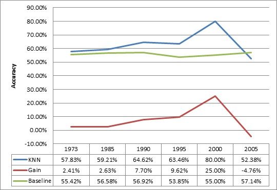
4.4.7 Summarized Results . . . . . . . . . . . . . . . . . . . . . . . . . 51
5 Conclusion and Future Work 53
5.1 Conclusion . . . . . . . . . . . . . . . . . . . . . . . . . . . . . . . . . . 53
5.2 Future Work . . . . . . . . . . . . . . . . . . . . . . . . . . . . . . . . . . 54
References 55List of figures 3.1 Total matches played by each ODI team . . . . . . . . . . . . . . . . . . . 12 3.2 Average Prior Performance . . . . . . . . . . . . . . . . . . . . . . . . . . 13 3.3 Pakistan vs. Australia . . . . . . . . . . . . . . . . . . . . . . . . . . . . . 15 3.4 Pakistan vs. Bangladesh . . . . . . . . . . . . . . . . . . . . . . . . . . . 16 3.5 Pakistan vs. Others . . . . . . . . . . . . . . . . . . . . . . . . . . . . . . 16 3.6 Pakistan vs. Zimbabwe . . . . . . . . . . . . . . . . . . . . . . . . . . . . 16 3.7 Pakistan vs. England . . . . . . . . . . . . . . . . . . . . . . . . . . . . . 17 3.8 Pakistan vs. South Africa . . . . . . . . . . . . . . . . . . . . . . . . . . . 17 3.9 Pakistan vs. West Indies . . . . . . . . . . . . . . . . . . . . . . . . . . . 17 3.10 Pakistan vs. New Zealand . . . . . . . . . . . . . . . . . . . . . . . . . . . 18 3.11 Pakistan vs. India . . . . . . . . . . . . . . . . . . . . . . . . . . . . . . . 18 3.12 Pakistan vs. Sri Lanka . . . . . . . . . . . . . . . . . . . . . . . . . . . . 18 3.13 Temperature distribution . . . . . . . . . . . . . . . . . . . . . . . . . . . 24 3.14 Humidity distribution . . . . . . . . . . . . . . . . . . . . . . . . . . . . . 25 3.15 Wind Speed distribution . . . . . . . . . . . . . . . . . . . . . . . . . . . 27 4.1 Attribute weights . . . . . . . . . . . . . . . . . . . . . . . . . . . . . . . 39 4.2 Stratified Sampling . . . . . . . . . . . . . . . . . . . . . . . . . . . . . . 41 4.3 Winning pattern of Pakistan against New Zealand . . . . . . . . . . . . . . 43 4.4 Results using setting 1 . . . . . . . . . . . . . . . . . . . . . . . . . . . . 45 4.5 Results using setting 2 . . . . . . . . . . . . . . . . . . . . . . . . . . . . 46 4.6 Results using setting 3 . . . . . . . . . . . . . . . . . . . . . . . . . . . . 47
xvi

4.7   Results using setting 4 . . . . . . . . . . . . . . . . . . . . . . . . . . . .   48
4.8   Results using setting 5 . . . . . . . . . . . . . . . . . . . . . . . . . . . .   49
4.9   Results using setting 6 . . . . . . . . . . . . . . . . . . . . . . . . . . . .   50
4.10 Collective results offered by each algorithm . . . . . . . . . . . . . . . . .     51
4.11 Accuracy and gain achieved using kNN . . . . . . . . . . . . . . . . . . .         51
List of tables

 3.1   Temperature distribution . . . . . . . . . . . . . . . . . . . . . . . . . . .    24
 3.2   Humidity distribution . . . . . . . . . . . . . . . . . . . . . . . . . . . . .   26
 3.3   Wind Speed distribution . . . . . . . . . . . . . . . . . . . . . . . . . . .     27
Chapter 1

Introduction

Analyzing time oriented data and forecasting are among the most imperative problems that

analysts face across many fields. It is one of the core topics of research in data mining.

The advent of the internet has created a wealth of electronic data that has simplified the

use of particularly large data-sets to categorize historical features that could independently

explain major portions of variation associated with an outcome. In this dissertation, different

approaches for a new time series prediction problem i.e. predicting the outcome of One-Day

International (ODI) cricket match has been presented. Although the process of using past

data to predict cricket match outcome has been explored previously in the literature, this

dissertation looks to expand upon the current literature by establishing a consistent statistical

approach that allows one to predict the match outcome with a greater accuracy than previously

shown. Moreover, Pakistan Cricket Board (PCB) could use the model to assess the merits of

certain strategies of play. The term strategy refers to the systematic plan of action taken by

a team e.g. the coin toss (the captain winning the toss has an important decision to make;
Chapter 1. Introduction                                                                          2

whether to bat or field first), Field placement, choosing bowlers, batting order, batting shot

selection and sharing the strike. Additionally, this study could help cricket analysts, media

and gamblers essentially to discover winning pattern of Pakistan cricket team against all

other oppositions and pre-match analysis.

1.1       Aims and Objectives

The primary aim of this thesis is to establish a consistent statistical approach to a new time

series prediction problem i.e. prediction the outcome of cricket match for Pakistan team

against all international oppositions. Winning a One-Day International (ODI) cricket match

depends on a number of factors related to scoring as well as the athletic strengths of the

playing teams. While some of these factors have been investigated in the literature, others

have yet to be explored.

   Secondly, decisiveness of a range of variables that could define the outcome of an ODI

cricket match has to be explored. In addition to that, influence of recent matches on the

prediction of match outcome was investigated. Therefore, this problem lies well in time

series forecasting domain. Following objectives were set to achieve the aims:

       To develop a dataset containing vital attributes that define match outcome.

       To determine type of sampling technique that improves the performance of classifica-
        tion model.

       To investigate the effect of different size of training and testing data sets on prediction
        accuracy.

       To identify a classification model that offers exceptional prediction accuracy.
Chapter 1. Introduction 3 1.2 The Game of cricket Cricket is a bat-and-ball game played between two teams of 11 players on a field at the center of which is a rectangular 22-yard long pitch. Each team takes it in turn to bat, attempting to score runs, while the other team fields; each turn is known as an innings. Currently cricket has three different Formats i.e. Test, ODI and Twenty20. With the passage of time, popularity of cricket has increased vastly. Cricket is extremely popular in India, Pakistan, Australia, England, South Africa, Sri Lanka, New Zealand, West Indies, Bangladesh and Zimbabwe [24]. The bowler delivers the ball to the batsman who attempts to hit the ball with his bat away from the fielders so he can run to the other end of the pitch and score a run. Each batsman continues batting until he is out. The batting team continues batting until ten batsmen are out, or a specified number of overs of six balls have been bowled, at this point, the teams switch roles and the fielding team comes in to bat [35]. In professional cricket the length of a game ranges from 20 overs per side to Test cricket played over five days. The laws of cricket are maintained by the International Cricket Council (ICC) and the Marylebone Cricket Club (MCC) with additional Standard Playing Conditions for Test matches and One Day Internationals [22]. Cricket was first played in southern England in or before the 16th century. By the end of the 18th century, it had developed to be the national sport of England. The expansion of the British Empire led to cricket being played overseas and by the mid-19th century, the first international match was held. ICC, the game’s governing body, has 10 full members [1]. A One-Day International (ODI) match, so called because each match is scheduled for
Chapter 1. Introduction                                                                       4

completion in only one day, is the most common type of cricket played on an international

level. ODI cricket is played between two teams of 11 players, each team plays one innings

and faces a limited number of overs, usually a maximum of 50 (300 deliveries). Since the

inception of ODI cricket, there have been various rule changes, although general principles

have remained the same. Both sides bat once with the aim in the first innings to score as

many runs as possible, and in the second innings to score more than the target set by the first

team. Because an ODI match is comprised of two different stages (batting & fielding) teams

are chosen in order to maximize performance in both areas. Generally a team will consist of

specialist batsmen and specialist bowlers, with better batsmen batting higher up the order.

Several constraints are imposed upon the fielding team, with no player being allowed to bowl

more than 10 overs, ensuring that at least five different bowlers are used to bowl the required

50 overs [35].

1.3     Motivation

Cricket is the second most popular sports in the world. Most popular could mean most

watched, most played or most revenue-generating sports. The ICC cricket World Cup is

the second largest single sporting event in the world (third if Olympics is also considered),

drawing a cumulative television audience of 2-3 billion people [24]. Even in Pakistan, nearly

every individual is a fan of cricket. This kind of popularity demands Pakistan cricket team to

deliver best in every match. This study can be used to benefit Pakistan Cricket Board (PCB).

Board, coach and captain can use this tool to shape their strategies and plans. For instance, if
Chapter 1. Introduction                                                                       5

tool predicts a WIN for coming match, they could go confident in ground with a proper game

plan and if it predicts a LOSS, they could adjust their strategies accordingly by being more

alert and careful while playing to turn the match in must win game. Moreover, this study will

help analysts to discover winning pattern of Pakistani team against all other oppositions.

1.4     Research Question

"Pakistan cricket team is going to play an ODI match against an international team, predict

                                     the match outcome"

1.5     Thesis Structure and Contribution

This thesis is organized as follows: This chapter, chapter 1, contains an introduction to and

describes the purpose of the research work. The chapter also discusses brief history and some

fundamental standard rules to play cricket. In the next chapter, chapter 2, presents overview of

related work found in literature. Chapter 3 provides a complete background of methodology

used in this study, selection criteria for target team, data collection, preprocessing, data

set formation and few renowned classification methods that were used for performance

comparison in this dissertation. Chapter 4 comprises of experimental details, attribute

selection criteria, sampling technique adopted for analysis, dataset organization, model

organization and results obtained with all six dataset settings. Chapter 5 concludes the whole

thesis and shares the avenues for future work.
Chapter 2 Literature Review Initially cricket was played in England four hundred year back. However, with the expansion of the British empire it was adopted in overseas countries. The first One-Day international (ODI) game was played in 1971 which led cricket to emerge as a very popular worldwide game and became the first sports to use statistics as a tool for illustration and comparison. Match data since the beginning of the ODI game is available. As an international sport, it is of little surprise that cricket has attracted more attention in the literature than other games. Nevertheless, the literature search found little related machine learning work particularly on cricket match outcome prediction. 2.1 Related Work One of the earlier published work on cricket was presented in [29], who explored whether a negative binomial distribution would be applicable to certain movements or performance in
Chapter 2. Literature Review                                                                 8

the game of cricket. The hazard function of top batsmen using a non-parametric approach

based on runs scored for assessing batting performance presented in [18]. A method of

calculation proposed in [9] to determine the optimal scoring rate which can be done at any

stage of the innings, along with an estimate of the total number of runs to be scored or the

chance of winning in the following innings of ODI match. Some studies, such as those

conducted in [12] showed that a modification of the Duckworth-Lewis resource table can be

used to quantify the magnitude of victory in ODI matches.

   It was found that most of these studies describe the factors affecting winning to break

ties in tournament standings but do not focus on the analysis of the factors with the goal of

predicting the probability of victory before the match. There are cases where the magnitude

of the victory is important. In fact, large sums of money are routinely wagered when it comes

to betting on the outcomes of ODI games as reported by [5]. With the use of D-L approach,

they showed this process can be readily modified to produce ’in the run’ predictions. The

match outcome however cannot be predicted until the match starts, moreover prediction

results change radically as match progresses.

   Some work could be found on match outcome prediction in [6]. He mainly investigated

the effect of Duckworth-Lewis method to predict the true winner and concluded that the

method does not have sufficient amount of information to predict the match outcome. While

he statistically studied few more factors just to explore their effects on match outcome,

others have yet to be investigated especially to predict the match outcome before it is played.

The work of [11] concludes that winning the toss at the outset of the match provides no

competitive advantage but playing on one’s home field does. This research however an
Chapter 2. Literature Review                                                                9

analysis focused on two factors that affect the team performance. A study established in [4]

that home teams generally enjoy a significant advantage. Using the relative batting and

bowling strengths of teams, together with parameters that are associated with common

home advantage, winning the toss and the establishment of a first-innings lead, they applied

multinomial logistic regression techniques to explore how these factors affect outcomes of

the test-matches. They also concluded that teams generally gain no winning advantage as a

result of winning the toss.

   Artificial neural networks used in [8] for predicting the outcome of multi (mainly three)

team tournaments. To train the neural networks they used match results for various matches

played by the teams in the past 10 years. This was done keeping an assumption that the

squads or teams haven’t changed much over the past 10 years. The domains used for training

and testing include overall performance in the tournament and in the final match of the

tournament. To predict a tournament’s outcome, they run the data through all the networks

and add up the score for each team. The team with the highest score is the winner. They

considered insufficient dataset to train the model as few tournaments are played every year.

Furthermore, the objective of this study is to predict the match outcome against all opponents

rather than two teams of the tournament. This work differs in methodology and use different

attributes as well.

   A model was proposed in [30] for predicting the game progression and outcome in one-

day cricket. They developed separate models for matches played by a team at home-ground

and other-grounds using historical and instantaneous features from past games. While Ridge

Regression and attribute bagging algorithms are used on the features to incrementally predict
Chapter 2. Literature Review                                                                 10

the runs scored in the innings. Their work is based on 125 matches played between January

2011 and July 2012 which obviously does not incorporate prior performance and possession

of any particular team. Even though prediction accuracy presented is not remarkable that

motivated us to explore this problem more deeply to further reduce the prediction error. A

Bayesian classifiers was used in [17], to predict how different attributes affect the outcome of

an ODI cricket match. The accuracy they achieved is deficient. Similar approach was carried

out further with some more useful attributes in order to get better accuracy.

   Some useful work can be found in [32] where thorough analysis of the Pakistan team,

as well as of several players was presented. The study might be helpful to understand the

particular conditions in which the Pakistan team is going to win (or lose), along with the

conditions in which a given batsman is going to score lesser or more runs. Despite using

satisfactory amount of attributes and dataset, they could not achieve significant accuracy as

far as prediction of match outcome is concerned.

   In whole literature review, it is found that quite little and average research has been

done to predict the match outcome. No work has been published with remarkable accuracy

yet. Those who applied comparatively good techniques, did not use most of the imperative

attributes. While others ignored the past data and took very small dataset that over fits the

model. At maximum 60% of accuracy was found in literature with several pitfalls in their

respective work. The aim was to gather all factual considerations presented in literature at

single point and come up with appropriate data set to drive smart attributes and effective

model.
Chapter 3

Methodology

Prediction model is chosen in order to guess the probability of an outcome on the basis of

given input dataset. Statistical analysis is usually performed using univariate and multivariate

analysis. Univariate analysis is the first phase in any statistical analysis and is used to

determine the direct relationship between individual variables and an outcome. Although

univariate tests give a decent indication to the strength and nature of the relationships of

interest, they are by no means conclusive. Consequently, analyst switch towards multivariate

model to further strengthen and validate results.

3.1     Background

Multivariate modeling is the optimal way used to maximize the information derived from

available dataset, and represents a standard approach adopted by most researchers in literature.

It is generally used to describe an analysis in which several variables are used simultaneously
Chapter 3. Methodology 12
to predict an outcome of interest. In this dissertation, the standard statistical approach used
in data-mining research has been applied to One-Day International (ODI) cricket. Three
features differentiate this work form most other’s; Firstly, the study focuses on training the
model according to time series forecasting that is how results of recent match can be used
to aid the prediction of match outcome. Secondly, effectiveness of consecutive wins as an
attribute was proposed and evaluated. Thirdly, it is the most comprehensive study conducted
in this area so far, covering a historical record of 34 years. The impact of different dataset
sizes on prediction accuracy was also investigated.
3.2 Target Team
The primary question arises before initiating analysis is that for which country the analysis
should be carried out. Since a large data set helps researchers to develop a better classification
model, teams who have played large no. of matches from its day one to 12th October, 2014
got the attention.
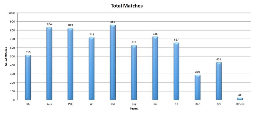
Fig. 3.1 Total matches played by each ODI teamChapter 3. Methodology 13
As shown in figure 3.1, only Pakistan, Australia and India have played 800+ matches so
far. Although India has played most matches, winning pattern of these three teams must be
analyzed in order to select most challenging problem.
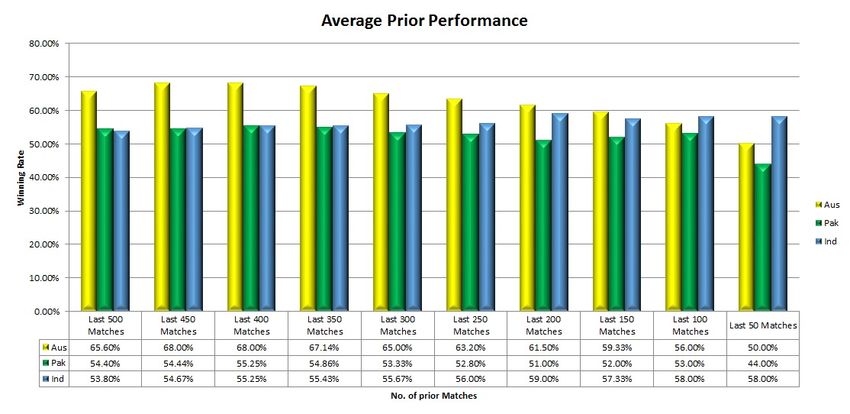
Fig. 3.2 Average Prior Performance
Figure 3.2 reveals some more useful information about these three teams. i.e., columns in
chart shows Pakistan won 44% matches in last 50 matches, 53% matches in last 100 matches,
52% matches in last 150 matches and so on. Though India and Australia have played more
matches than Pakistan, both have growing and decaying winning pattern respectively. In
other words, match outcome is somehow less uncertain for both teams. Whilst Pakistan has
most uncertain behavior as far as match outcome is concerned. It has almost 50% chance of
winning in throughout ODI matches, this behavior is even worst in last 50 matches. SinceChapter 3. Methodology 14
test set will be comprising of most recent matches, learning an appropriate classification
model could be more interesting and challenging. Therefore, Pakistan team has been selected
for this study.
3.3 Winning Pattern of Pakistan against each Team
Following graphs illustrate a rough idea about winning pattern of Pakistan against each
opponent. Since single model for all opponents was learned, this analysis helps to make some
useful assumptions. Rule to make these graphs is simple, start with zero and +1 for each
win and -1 for each lose. Y-axis is for winning pattern and X-axis for number of matches
played. Rise in graph shows consecutive wins and fall shows successive losses. This analysis
also useful in setting priorities for individual opponents while tuning the absolute model. In
other words only those attributes and model’s parameters were select that gives best accuracy
against opponents having high priority.
When Australia is considered as an opponent, it can be seen in figure 3.3 that Pakistan
has a random performance behavior in first 35 matches then they lose mostly. Therefore, this
opponent was considered as important one in order to learn best possible model against such
irregular behavior.
While Bangladesh, Others and Zimbabwe are considered as an opponent, it can be seen
in figure 3.4, 3.5, 3.6 that Pakistan has been consistently winning against these particular
opponents. Therefore, even a simple model can give the better performance. This opponent
was kept at least priority while learning the overall model.Chapter 3. Methodology 15
While considering England, South Africa and West Indies as opponents, it can be seen
in figure 3.7, 3.8, 3.9 that Pakistan has not been consistent against them. Therefore, this
opponent was kept at moderate priority while learning the overall model. However, large
number of losses helped in tuning the model effectively.
While considering New Zealand, India and Sri Lanka as opponents, it can be seen in
figure 3.10, 3.11, 3.12 that Pakistan has not been consistent against them too. Therefore,
this opponent was kept at moderate priority while learning the overall model. However,
comparatively large number of wins assist to tune the model accordingly.
Fig. 3.3 Pakistan Vs. AustraliaChapter 3. Methodology 16
Fig. 3.4 Pakistan Vs. Bangladesh
Fig. 3.5 Pakistan Vs. Others
Fig. 3.6 Pakistan Vs. ZimbabweChapter 3. Methodology 17
Fig. 3.7 Pakistan Vs. England
Fig. 3.8 Pakistan Vs. South Africa
Fig. 3.9 Pakistan Vs. West IndiesChapter 3. Methodology 18
Fig. 3.10 Pakistan Vs. New Zealand
Fig. 3.11 Pakistan Vs. India
Fig. 3.12 Pakistan Vs. Sri LankaChapter 3. Methodology 19 3.4 Dataset Data collection is one of the most important steps in any machine-learning problem. Data should be as large as possible and have enough correlation with the labels, to serve well for the given problem. The prime difficulty in ODI outcome prediction problem is to collect a vast variety of data to form a single dataset on which the model can be learned. The outcome of a cricket match depends on various factors like season in which match played, opponent team, country, venue ground, match format(Day/Night), batting order(First/Second), recent form of the team(Consecutive wins), team selection and utiliza- tion of players. The outcome can also vary due to some key weather attributes like event (sunny/rain/fog), wind speed, humidity and temperature that ultimately define the Pitch behavior. 3.4.1 Data Collection The prime source of data were [2] & [3]. Separate dataset was established for each team which consists following attributes: ODI no. as an identifier, Date of the match, opponent team, batting first or not, whether match is Day/Night match or not, Ground and country of the match played, score, runs per over, and wickets fallen in first and second innings of the match, the margin of victory (in terms of runs if the team batting first has won the match or number of wickets in hand and balls remaining, in case the team batting second has won the match). Also data contains a binary label Result which is 0 in case of a lost match and 1 otherwise. A match that results in a draw or had no result or was abandoned is not included
Chapter 3. Methodology                                                                        20

in the dataset..

    Eleven (11) different datasets has been made for ODI format, which includes a dataset

for each of the 10 test playing countries. The 11th dataset is a merged dataset of all non-test

playing countries named as others. Merging non-test playing teams which are not so mature

in cricket is logical since these teams have similar(i.e. weak) behavior against test playing

teams. Dataset was developed for all ODI matches, i.e. matches played since 1971 (upto

12-oct-2014). This adds up to three thousand and thirty four matches(i.e. 3534) divided

into eleven different data set sheets. India has the largest dataset with 863 matches and

Bangladesh has the least dataset of 290 matches.

3.5     Preprocessing

Collected data was pre-processed and trimmed in order to mold the raw data in such a way

that it gets a form of useful dataset. Since the prime objective of this study was the prediction

of ODI match outcome for Pakistan as Win/Lose, all matches played against any team by

Pakistan were incorporated to form a dataset. Opponent countries like Australia, South

Africa, England, India, New Zealand, West Indies, Bangladesh, Sri Lanka, and Zimbabwe

are treated as individual teams and rest as others (e.g. Ireland, Canada etc.). The following

subsections present details of all respective attributes based on literature search and the

criteria adopted for their construction in this study.
Chapter 3. Methodology 21 3.5.1 Home advantage The role of home advantage (HA) has been shown to play a vital role in any analysis of sporting events. The notion of HA has long been renowned as a known phenomenon in sport and has been origin for much research. Some useful work can be found in [11] that winning the coin toss at the outset of a match provides no competitive advantage whereas the advantages of playing one’s home field increase the probability of winning in ODI match. In spite of the fact that different approaches have been used to quantify HA, the underlying reason why HA exists has been reduced to three basic principles: 1. Travel 2. Familiarization and 3. Crowd support Study in [31] confirms the existence of a home advantage in organized sports. They presented that more effective offensive rather than defensive action is the major factor in the home advantage among various sports. They further showed inferences from the data, as well as more direct observations on audience size and its relationship to performance and outcome, justifying the conclusion that the home advantage is almost totally independent of visitor fatigue and lack of familiarity with the home playing area; it is mainly attributable to the social support of the Crowd. Therefore in this dissertation, a high priority was given to this particular attribute of home advantage.
Chapter 3. Methodology                                                                    22

3.5.2    Pitch Report

Another important attribute in the prediction of a cricket match is the pitch report. Unfor-

tunately, the pitch report of each match is not available in any kind of record. Therefore,

the behavior of the pitches of all the venues was generalized, as the pitch behavior almost

remains consistent with respect to time. Slight variations as the presence of amount of grass

and cracks on the pitch may vary on a given day but overall behavior remains same. Careful

observations from analysis of key analysts and their articles were made. The pitch behaviors

were classified into slow, bouncy, dry and green pitches. After careful study of pitches, a

pitch type to all of the one hundred and Fifty Seven (157) international cricket grounds were

assigned.

3.5.3    Weather Report

Beside match and ground attributes weather also plays a vital role on the outcome of the

match. Especially the temperature, overcast and humidity (which results in due factor in

day/night matches) has a vital impact on the outcome of cricket matches. Weather data was

collected for 150 cities that spreads overs 6 continents. This data is available from 1996

only. However, data for few cities (like Hyderabad, Chandigarh, Bangalore, Dambulla) were

not available on weather underground website, for such cities data was taken from nearest

weather stations. Since weather attributes are continuous in nature, reasonable preprocessing

on data was required. Therefore, standard discretization techniques were applied to transform

continuous models into discrete counterparts.
Chapter 3. Methodology                                                                          23

Overcast

In cricket, a rain-affected pitch can make batting more difficult than normal. Several other

conditions such as poor light or an initially lively pitch, may also result in difficulties for the

batsmen [26]. Therefore, Overcast of each city was considered in this study and discretized

as rainy, sunny and cloudy.

Temperature

In one-day cricket the work rate, although stops and starts at irregular intervals, can at times

be fairly intense resulting in the generation of a considerable amount of heat in human body.

The nature of the activity combined with stressful environmental conditions, common in

many cricket-playing countries, is likely to increase the thermal load placed on the body

of players as reported in [19]. Consequently, field temperature strongly affect the match

outcome, hence considered in this study. Since the temperature information is available from

1996, only 419 out of 824 matches have temperature information in the dataset. Using IBM

SPSS tool, the temperature data was statistically analyzed over 419 matches in order to have

an idea about temperature range/distribution of all matches in figure 3.13.
Chapter 3. Methodology                                            24

                         Fig. 3.13 Temperature distribution

                   N                                        419
                   Mean                                   22.58
                   Median                                 23.00
                   Mode                                   28.00
                   Std. Deviation                          6.11
                   Variance                               37.43
                   Range                                     30
                   Minimum                                    7
                   Maximum                                   37

                                            25            18.00
                   Percentile               50            23.00
                                            75            28.00
                         Table 3.1 Temperature distribution
Chapter 3. Methodology 25
Results in table 3.1 reveals some useful information about temperature distribution in
overall dataset. Hence, the temperature was categorized as follows:
Temperature ≤ 18C : Low
28C < Temperature < 18C : Normal
Temperature ≥ 28C : High
Humidity
Humidity indicates the likelihood of precipitation, dew, or fog. Higher humidity reduces
the effectiveness of sweating in cooling the body by reducing the rate of evaporation of
moisture from the skin. This factor can also affect the match outcome because precipitation
defines how quick or slow the field is, dew effects bowling and fielding and fog could be even
worse [15]. Therefore same is the case with Humidity; the data was statistically analyzed for
discretization using IBM SPSS tool in figure 3.14.
Fig. 3.14 Humidity distributionChapter 3. Methodology 26
N 419
Mean 65.01
Median 67.00
Mode 75.00
Std. Deviation 15.56
Variance 242.25
Range 86
Minimum 12
Maximum 98
25 56.00
Percentile 50 67.00
75 76.00
Table 3.2 Humidity distribution
According to information available in table 3.2, Humidity was categorized as follows:
Humidity ≤ 56 : Low
56 < Humidity < 76 : Normal
Humidity ≥ 76 : High
Wind Speed
Wind speed directly affect the player’s performance hence the match outcome [15]. Same is
the case with wind speed, the data was statistically analyzed for discretization using IBM
SPSS tool in figure 3.15.Chapter 3. Methodology 27
Fig. 3.15 Wind Speed distribution
N 419
Mean 11.58
Median 11.00
Mode 10.00
Std. Deviation 4.41
Variance 41.17
Range 31
Minimum 0
Maximum 31
25 7.00
Percentile 50 11.00
75 16.00
Table 3.3 Wind Speed distributionChapter 3. Methodology 28
According to information available in table 3.3, Wind Speed was categorized as follows:
WindSpeed ≤ 7km/h : Low
7km/h < WindSpeed < 16km/h : Normal
WindSpeed ≥ 16km/h : High
3.5.4 ODI#
ICC One Day International number was considered to aid time series forecasting in learning
the model. It has direct relation with recent matches; an example with higher value of ODI
represents the latest match. This attribute was considered in different forms i.e.
Actual form
Normalized form 0 to 12
Normalized form 0 to 1
To aid model in different ways (discussed later in dissertation). However, only one type of
ODI is used as attribute to learn a particular model.
3.5.5 Date
Date of the day, match was played on. It is considered to aid time series forecasting in
learning the model too. It also has direct relation with recent matches, an example with latest
date represent the latest match. This attribute was also considered in quit different forms i.e.
Actual form 02111973 (ddmmyyyy)
Modified date 19731102 (yyyymmdd)Chapter 3. Methodology 29
Date with Linear Weight 0 to 1
Date with Non Linear Weight 0 to 115856201
Year 1973
Year 0 to 1
Year 0 to 12
to aid model in different ways(discussed later in dissertation). However, only one type of
date is used as attribute to learn a particular model.
3.5.6 Season
Season or month, the match was played in. It effectively contributes to define match outcome
since all-weather conditions get changed in every season (e.g. winter, spring, summer and
autumn). It incorporates temperature, humidity, wind conditions etc, in unaided manner. This
attribute was considered in quite different forms i.e.
All 12 months in an individualistic manner
Months divided into 4 categories
Months divided into 3 categories
Season (winter, spring, summer and autumn)
to aid model in different ways(discussed later in dissertation). However, only one type of
form is used as an attribute to learn a particular model.Chapter 3. Methodology 30 3.5.7 Opposition The opponent, played the match against Pakistan. All non-test playing teams or new teams are grouped and named as others, since these teams have similar (i.e. weak) behavior against test playing teams. 3.5.8 Country Location where the match was played, considered in its actual form. 3.5.9 Ground Venue where the match was played, considered in its actual form. 3.5.10 Day/Night Match type (day or day & night), considered in its actual form and categorized as Yes/No. 3.5.11 Batting First Tells whether Pakistan bated first or not), considered in its actual form and categorized as Yes/No.
Chapter 3. Methodology                                                                        31

3.5.12     Consecutive Wins before Current Match

The count of consecutive wins for Pakistan before the current match is played. It is an integer

type of attribute and being considered for the first time to predict the match outcome in

One-day International (ODI).

3.5.13     Pak Win

It is a target label, Tells whether Pakistan Won the match or loosed, categorized as Yes/No.

3.6      Classification Methods

In machine learning, classification is the process of identifying the class of a new observation

based on a training set containing observations with known classes. Classifier’s performance

highly depends on the characteristics of the data to be classified. Although there is no single

classifier that works best in every application, determining an appropriate classifier for a

given scenario is however still more an art than a science. In spite of the fact that vast verity

of classifiers exists in literature, six classifiers were short-listed for performance comparison

in this dissertation. Selected classifiers are not only among the most influential data mining

classifiers in the research community but also highly diverse in nature.

3.6.1    k-Nearest Neighbors

K-nearest-neighbor (kNN) is one of the most fundamental and simple classification methods

and should be,first choices for a classification study when there is little or no prior knowledge
Chapter 3. Methodology                                                                       32

about the distribution of the data. K-nearest-neighbor classification was developed from

the need to perform discriminant analysis when reliable parametric estimates of probability

densities are unknown or difficult to determine [28].

   The algorithm is commonly based on the Euclidean distance between a test sample and

the specified training samples. In order to decide which of the points from the training dataset

are similar enough to be considered when choosing the class for a new observation is to

pick the k closest data points, and to take the most common class among these. Hence, an

example is classified by majority vote of its neighbors.

   K-nearest-neighbor is a versatile algorithm, used in a huge number of fields. Content

retrieval, gene expression, protein-protein interaction and 3D structure prediction lie in few

uncommon and non trivial applications of kNN.

3.6.2    Artificial Neural Network

An Artificial Neural Network (ANN) is an information-processing model that is inspired by

the way a nervous system (brain) process information. Large number of highly interconnected

processing elements (neurons) work in unison to solve a specific problem. Its flexible

mathematical structure is capable of identifying complex nonlinear relationships between

input and output data sets [16].

   ANN models have been found useful and efficient, particularly in problems for which the

characteristics of the processes are difficult to define using physical equations. The utility

of artificial neural network models lies in function approximation, or regression analysis,
Chapter 3. Methodology                                                                         33

including time series prediction, classification, including pattern and sequence recognition

and computer numerical control etc.

3.6.3    Decision Trees

Decision tree is a method for approximating discrete-valued functions that is robust to noisy

data and capable of learning disjunctive expressions. The learned function can be represented

as tree-shaped diagram or as sets of if-then-else rules to improve human readability. Decision

tree classify instances by sorting them down the tree from the root to some leaf node, which

provides the classification of the test instance [23]. In fact, the most important feature of

decision tree is its capability to break down a complex decision-making process into a group

of simpler decisions, thus providing a solution that is often easier to interpret. It lies among

the most popular of inductive inference algorithms and have been successfully applied to a

broad range of tasks from diagnose medical cases to assess credit risk of loan applicants.

3.6.4    Random Forest

Random forest is a learning method used for classification and regression. It grows many

classification trees then puts the input vector down each of the trees in the forest to classify a

new instance. Each tree gives a classification of a label (target variable), and it is called the

tree "votes" for that class. The forest chooses the classification having the most votes in whole

trees of the forest [21]. Random forest works efficiently with high dimensional datasets and

gives estimate to identify vital attributes in the classification. It precludes decision tree’s

habit of over-fitting to the training set.
Chapter 3. Methodology                                                                        34

   In particular, trees that are grown very deep, tend to learn extremely irregular patterns:

they over-fit the training set, because they have low bias, but very high variance. Random

forest provides a way of averaging multiple deep decision trees, trained on different parts of

the same training set, with the goal of reducing the variance [14]. This comes at expense of a

slight rise in the bias and certain loss of interpretability, but offers significant boost in the

performance of the final model.

3.6.5    Logistic regression

Logistic regression measures relationship between the categorical dependent variable and

one or more independent variables by estimating probabilities. It deals with conditions in

which the observed outcome for a dependent variable can have only two possible types [13].

Logistic regression is widely used in many fields. Such as in medical, to predict mortality in

injured patients [7]; in engineering to predict the probability of failure of a given process,

system or product [27]; in marketing applications prediction of a customer’s propensity to

purchase a product or halt a subscription and in business applications to predict the likelihood

of a homeowner defaulting on a mortgage have been developed using logistic regression.

3.6.6    Naïve Bayes

Naïve Bayes provides a reliable probabilistic approach for inference. It is based on applying

Bayes theorem with strong (naive) independence assumption that is all the features are

conditionally independent given the class label. Even though this is usually incorrect (since

features are usually dependent), the resulting model is easy to fit and works remarkably
Chapter 3. Methodology                                                                 35

well in many applications [25]. Naive Bayes has proven its effectiveness in many practical

applications, including text classification, medical diagnosis, and systems performance

management.
Chapter 4

Experimental Details and Results

4.1     Attribute Selection

The recent detonation of data set size, in number of examples and attributes, has triggered

the development of a number of big data platforms. At the same time though, it has pushed

for usage of data dimensionality reduction techniques. Indeed, more is not always better. Big

data sometimes produce worse performances in data analytics applications [34]. Therefore,

it is better to use smart attributes with simple models for classification than smart model with

high dimensional data. Thus, identifying most adequate attributes to predict match outcome

was the most critical milestone of this study.

   In first phase, attributes having missing values are eliminated manually. For example,

attributes like temperature, humidity, overcast and wind speed has data of only 419 out of

823 ODI matches (from 1996), due to insufficient data these attributes are eliminated for this
Chapter 4. Experimental Details and Results                                                  38

study. However, feature engineering techniques has been applied on few attributes which

ended up with following attributes:

   1. Country                                     10. Season

   2. Ground                                             (a) All 12 months in an individualis-
                                                             tic manner
   3. Day/Night
                                                        (b) Months divided into 4 categories
   4. Batting First
                                                         (c) Months divided into 3 categories
   5. Pitch Report                                      (d) Season (winter, spring, summer
   6. Home Ground                                           and autumn)

   7. Consecutive Wins before Current             11. Date
      Match
                                                         (a) Actual form 02111973 (ddm-
       (a) Actual form                                       myyyy)
       (b) Normalized form 0 to 1                       (b) Modified form 19731102 (yyyym-
                                                            mdd)
   8. Opposition
                                                         (c) Date with Linear Weight 0 to 1
       (a) 18 opponents                                 (d) Date with Non Linear Weight 0
       (b) 10 opponents                                     to 115856201
   9. ODI#                                               (e) Year 1973
                                                         (f) Year 0 to 1
       (a) Actual form
                                                        (g) Year 0 to 12
       (b) Normalized form 0 to 12
       (c) Normalized form 0 to 1                 12. Pak Win

   In second phase, attribute’s weights were computed using “Weight by Relief” operator

available in Rapid Miner software tool. This operator computes the relevance of the attributes

by Relief. Relief is a feature selection algorithm which selects the relevant features using

statistical method. Although, relief does not depend on heuristics, it is accurate and noise-

tolerant even if features interact. It requires only linear time in the number of given features

and training instances, regardless of the target concept complexity [20].
Chapter 4. Experimental Details and Results 39
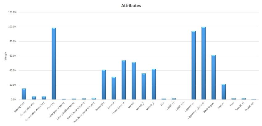
This exercise was done to select form of an attribute that contributes well in defining the
outcome among its other forms(e.g. season, ODI# and date etc). Figure 4.1 depicts calculated
weight of each attribute.
Fig. 4.1 Attribute weights
In order to ensure that only one attribute of each category is to be considered, attributes
are short listed on the basis of their respective weights. However, attributes having only
single form (e.g country, ground and pitch report etc.) were considered as it is. Following are
the short listed attributes:
1. Batting First 6. Ground
2. Consecutive Wins Before Current 7. Home Ground
Match
8. Month-4
3. Country
9. ODI(0-1)
4. Date Non-Linear Weight
10. Opposition(Others)
5. Day/Night
11. Pitch ReportChapter 4. Experimental Details and Results 40
A dataset may contain attributes that provide little power to classify instances even in
some cases, these attributes negatively affect the classification accuracy. Therefore, in order
to eliminate such attributes the brute-force algorithm was used in this final phase of data
dimensionality reduction process. The brute-force search also known as exhaustive search, is
an attribute selection method that evaluate all possible combinations of the input features,
and then find the best subset.
While a brute-force search is easier to implement, and will always find a best possible
solution (if it exists), its cost is proportional to the number of attributes, which in many
practical problems tends to grow very quickly as the number of attributes increases(Even
15 attributes cause 32768 iteration in brute force). Therefore, brute-force search is typically
used when the number of attributes are limited, or the simplicity of implementation is more
important than speed [33].
Since the target problem satisfies both condition, brute-force technique was used to
identify the best attributes to learn prediction model using top 6 classifiers including KNN,
Neural Network, Decision Tree, Random Forest, Logistic Regression and Naïve Bayes. It
is found that 5 attributes give best performance with every classification model hence they
are finally selected for further analysis taking different data set sizes. Those 5 attributes are
listed below:
1. Consecutive Wins Before Current Match
2. Opposition (Others)
3. Ground
4. Home Ground
5. Day/NightChapter 4. Experimental Details and Results 41
4.2 Sampling Technique
Stratified sampling criteria was used in order to split data into training and testing sets.
In statistics, stratified sampling is a technique of dividing members of the population into
homogeneous subgroups before sampling. It is advantageous to sample each subpopulation
independently when subpopulations within an entire population vary. Proportionate allocation
uses a sampling fraction in each of the subpopulation that is proportional to that of the entire
population [10]. For instance, if the population S consists of m examples in the male subpop-
ulation and f examples in the female subpopulation (where m + f = S), then the relative size
of the two samples (x1 = m/S*testset size, x2 = f/S*testset size) should reflect this proportion.
Fig. 4.2 Stratified Sampling
Such as, in figure 4.2 there are twice as many males as females in a population. Therefore,
there will be twice as many males as females in a stratified sample for the testset size of 6Chapter 4. Experimental Details and Results 42 instances. The subpopulation should be mutually exclusive and collectively exhaustive. With stratified sampling, the examiner can representatively sample even the smallest and most inaccessible subgroups in the population. This enables one to sample the rare extremes of the given population which suits our case. The technique offers higher statistical precision compared to simple random sampling because the variability within the subgroups is lesser compared to the variations when dealing with the entire population. 4.3 Experimental Setup Only single model was learned to predict match outcome against all opponents. Since opposition was considered as mandatory attributes in every classification model learning, classifier had enough capability to disregard instances belong to all opposition except the one (which lies in test instance) in classification process. 4.3.1 Dataset Organization Despite the fact that data is available from January 1970, Due to the continuous modification in cricket rules, earlier matches should be disregard for better results. Obviously, with the passage of time, teams get matured and develop strengths in all areas (batting, bowling and fielding) with experience. Even today’s match outcome is highly influenced by strategies and technicality measures embraced by a particular team. For instance, Pakistan could not capture most wins in early 30 matches i.e. Pakistan lost most of the matches before 1992 then in figure 4.3 an incredible performance can be seen by Pakistan against the same opponent.
Chapter 4. Experimental Details and Results                                                 43

                 Fig. 4.3 Winning pattern of Pakistan against New Zealand

   Since Pakistan has now become a highly matured and competitive team, in order to

classify new matches, earlier instances should be excluded when Pakistan were in armature

phase in the game of cricket. Moreover, rapid changes in game rules also encourage one to

ignore those matches which loses correlation from today’s one in terms of game rules. But

the question is who many matches to be ignored? Because winning rate not only varies with

opponent to opponent but also a team do has a psychological pressure/confidence of its prior

performance associated every opponent. Therefore, datasets with following intervals were

investigated to find optimal one for final model. (Results obtained using each dataset size are

shown in next section)

   1. Dataset form 1973 to present

   2. Dataset form 1985 to present

   3. Dataset form 1990 to present

   4. Dataset form 1995 to present
Chapter 4. Experimental Details and Results 44 5. Dataset form 2000 to present 6. Dataset form 2005 to present 4.3.2 Model Organization In each technique the dataset was divided into training, validation and test set for every classification model. The 75% dataset was used to construct training set in order to train the classification model. Whereas 15% dataset was used to construct validation set. Validation set, which is independent from the training set, is used for model’s parameter tuning/selection and to avoid over fitting. The rest 10% dataset, which was absolutely unseen to the prediction model (like future matches), was used to evaluate the performance of the trained model. However, after parameter tuning, validation set was then merged with training set to form a new training set of 90% examples for performance evaluation. While evaluating classification model, performance was compared with baseline too to highlight the gain factor.
Chapter 4. Experimental Details and Results 45
4.4 Results
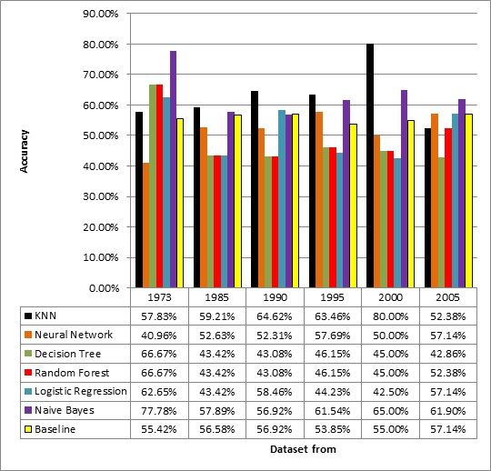
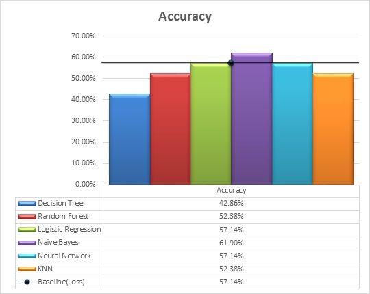
4.4.1 Setting 1
In this first setting, whole dataset from 1973 to 2014 was considered with 5 attributes men-
tioned in previous section. All classification algorithms are used with their default parameters.
The dataset contains following characteristics:
Fig. 4.4 Results using setting 1
Result in figure 4.4 shows that the Naïve Bayes outperforms all other classification
algorithms with performance gain of 22.36% w.r.t baseline.Chapter 4. Experimental Details and Results 46
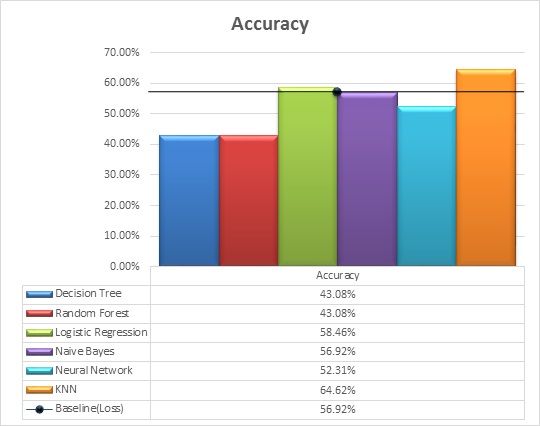
4.4.2 Setting 2
In this second setting, dataset from 1985 to 2014 was considered with same attributes and
default parameters of all classification algorithm. The dataset contains following characteris-
tics:
Total no. matches : 749
No. of Examples in Training set (90%) : 673
No. of Examples in Test set (10%) : 76
Fig. 4.5 Results using setting 2
Result in figure 4.5 shows that the K Nearest Neighbor (kNN) outperforms all other
classification algorithms with performance gain of 2.63% w.r.t baseline.You can also read