A Multi-view CNN-based Acoustic Classification System for Automatic Animal Species Identification
←
→
Page content transcription
If your browser does not render page correctly, please read the page content below
A Multi-view CNN-based Acoustic Classification System for Automatic
                                                                Animal Species Identification

                                                                       Weitao Xua , Xiang Zhangb , Lina Yaob , Wanli Xueb , Bo Weic
                                                                 a Department of Computer Science, City University of Hong Kong, Hong Kong
                                                            b Schoolof Computer Science and Engineering, University of New South Wales, Australia
                                                               c Department of Computer and Information Sciences, Northumbria University, UK
arXiv:2002.09821v1 [eess.AS] 23 Feb 2020

                                           Abstract
                                           Automatic identification of animal species by their vocalization is an important and challenging task. Al-
                                           though many kinds of audio monitoring system have been proposed in the literature, they suffer from several
                                           disadvantages such as non-trivial feature selection, accuracy degradation because of environmental noise or
                                           intensive local computation. In this paper, we propose a deep learning based acoustic classification frame-
                                           work for Wireless Acoustic Sensor Network (WASN). The proposed framework is based on cloud architecture
                                           which relaxes the computational burden on the wireless sensor node. To improve the recognition accuracy,
                                           we design a multi-view Convolution Neural Network (CNN) to extract the short-, middle-, and long-term de-
                                           pendencies in parallel. The evaluation on two real datasets shows that the proposed architecture can achieve
                                           high accuracy and outperforms traditional classification systems significantly when the environmental noise
                                           dominate the audio signal (low SNR). Moreover, we implement and deploy the proposed system on a testbed
                                           and analyse the system performance in real-world environments. Both simulation and real-world evaluation
                                           demonstrate the accuracy and robustness of the proposed acoustic classification system in distinguishing
                                           species of animals.
                                           Keywords: Wireless acoustic sensor network, Animal identification, Deep learning, CNN

                                           1. Introduction                                               the inadvertent introduction of the Asian Longhorn
                                                                                                         Beetle has cost USA government millions of dollars
                                              Wireless Acoustic Sensor Network (WASN)                    to eradicate the Beetle population [5]. Therefore, a
                                           based animal monitoring is of great importance for            wireless monitoring system is imperative to detect
                                           biologists to monitor real-time wildlife behavior for         the distribution of these insects.
                                           long periods and under variable weather/climate                  There are a large volume of audio monitoring sys-
                                           conditions. The acquired animal voice can pro-                tems in the literature [4, 6, 7, 8, 9, 10, 11, 12, 13, 14].
                                           vide valuable information for researchers, such as            In the early stage, biologists have traditionally de-
                                           the density and diversity of different species of an-         ployed audio recording systems over the natural en-
                                           imals [1, 2, 3]. For example, Hu et al. proposed a            vironment where their research projects were de-
                                           WASN application to census the populations of na-             veloped [6, 7]. However this procedure requires
                                           tive frogs and the invasive introduced species (Cane          human presence in the area of interest at certain
                                           Toad) in Australia [4]. There are also several im-            moments. In recent years, with the development
                                           portant commercial applications of acoustic animal            of WSN, some researchers have proposed remotely
                                           detection. For instance, America imports billions             accessible systems in order to minimize the impact
                                           of dollars of timber from Aisa every year. However,           of the presence of human beings in the habitat of
                                                                                                         interest [4, 12, 13, 14].
                                                                                                            Despite much effort in this area, previous stud-
                                               Email addresses: weitaoxu@cityu.edu.hk (Weitao
                                           Xu), xiang.zhang3@student.unsw.edu.au (Xiang Zhang),
                                                                                                         ies suffer from several disadvantages. First, tradi-
                                           lina.yao@unsw.edu.au (Lina Yao), w.xue@unsw.edu.au            tional methods usually first extract a number of ap-
                                           (Wanli Xue), bo.wei@northumbria.ac.uk (Bo Wei)                propriate features and then employ classic machine
                                           Preprint submitted to Elsevier                                                                        February 25, 2020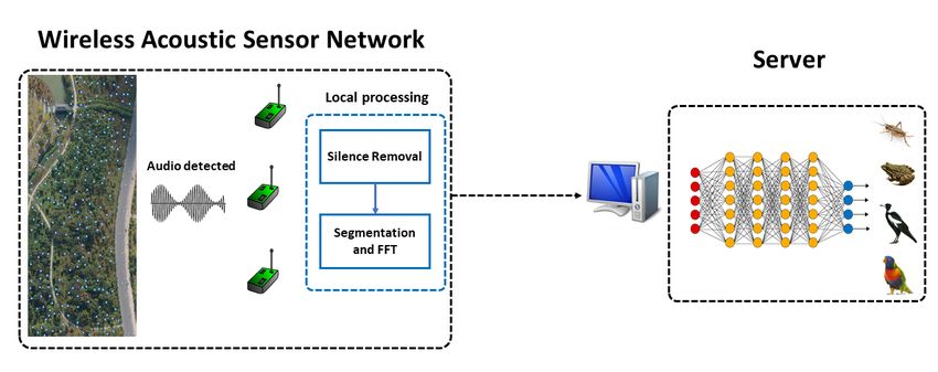
learning methods such as Support Vector Machine                  Recently, deep learning has emerged as a pow-
(SVM) or K-Nearest Neighbours (KNN) to detect                 erful tool to solve various recognition tasks such
the species of the animals. Features, such as sta-            as face recognition [18], human speech recogni-
tistical features through statistical anlaysis (e.g.,         tion [19, 20] and natural language processing [21].
variance, mean, median), Fast Fourier Transmis-               The application of deep learning in audio signal
sion (FFT) spectrum, spectrograms, Wigner-Ville               is not new; however, most previous studies focus
distribution (WVD), Mel-frequecy cepstrum coef-               on human speech analysis to obtain context infor-
ficient (MFCC) and wavelets have been broadly                 mation [19, 20, 22]. Limited efforts have been de-
used. However, extracting robust features to rec-             voted to applying deep learning in WASN to clas-
ognizing noisy field recordings is non-trivial. While         sify different species of animals. To bridge this gap,
these features may work well for one , it is not clear        we aim to design and implement a acoustic classi-
whether they generalize to other species. The spe-            fication framework for WASN by employing deep
cific features for one application do not necessarily         learning techniques. Convolutional Neural Network
generalize to others. Moreover, a significant num-            (CNN), as a typical deep learning algorithm, has
ber of calibrations are required for both manually            been widely used in high-level representative fea-
feature extraction and the classification algorithms.         ture learning. In detail, CNN is enabled to capture
This is because the performance of the traditional            the local spatial coherence from the input data. In
classifiers such as SVM and KNN [8, 10, 11] highly            our case, the spatial information refers to the spec-
depends on the quality of the extracted features.             tral amplitude of the audio signal. However, one
However, handcrafting features relies on a signifi-           drawback of the standard CNN structure is that the
cant amount of domain and engineering knowledge               filter length of the convolution operation is fixed.
to translate insights into algorithmic methods. Ad-           As a result, the convolutional filter can only dis-
ditionally, manual selection of good features is slow         cover the spatial features with the fixed filter range.
and costly in effort. Therefore, these approaches             For example, CNN may explore the short-term fea-
lack scalability for new applications. Deep learn-            ture but fail to capture the middle- and long-term
ing technologies can solve these problems by using            features. In this paper, we propose a multi-view
deep architectures to learn feature hierarchies. The          CNN framework which contains three convolution
features that are higher up in deep hierarchies are           operation with three different filter length in par-
formed by the composition of features on lower lev-           allel in order to extract the short-, middle-, and
els. These multi-level representations allow a deep           long-term information at the same time. We con-
architecture to learn the complex functions that              duct extensive experiments to evaluate the system
map the input (such as digital audio) to output               on real datasets. More importantly, we implement
(e.g. classes), without the need of dependence on             the proposed framework on a testbed and conduct
manual handcrafted features.                                  a case study to analyse the system performance in
   Secondly, these approaches suffer from accuracy            real environment. To the best of our knowledge,
degradation in real-world applications because of             this is the first work that designs and implements
the impact of environmental noise. The voice                  a deep learning based acoustic classification system
recorded from field usually contains much noise               for WASN.
which poses a big challenge to real deployment                   The main contributions of this paper are three-
of such system. To address this problem, Wei et               fold:
al. [15] proposed an in-situ animal classification sys-
                                                                • We design a deep learning-based acoustic clas-
tem by applying sparse representation-based classi-
                                                                  sification framework for WASN, which adopts a
fication (SRC). SRC uses `1 -optimization to make
                                                                  multi-view convolution neural network in order
animal voice recognition robust to environmental
                                                                  to automatically learn the latent and high-level
noise. However, it is known that `1 -optimization
                                                                  features from short-, middle- and long-term au-
is computationally expensive [16, 17], which limits
                                                                  dio signals in parallel.
the application of their system in resource-limited
sensor nodes. Additionally, in order to make SRC                • We conduct extensive evaluation on two real
achieve high accuracy, a large amount of training                 dataset (Forg dataset and Cricket dataset) to
data is required. This means a wireless sensor node               demonstrate the classification accuracy and ro-
can only store a limited number of training classes               bustness of the proposed framework to environ-
because of the limited storage.                                   mental noise. Evaluation results show that the
                                                          2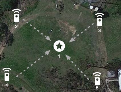
proposed system can achieve high recognition              realize in-network classification system because of
    accuracy and outperform traditional methods               the limited computational ability of wireless sensor
    significantly especially in low SNR scenarios.            node. Recently, several research works regarding
                                                              in-network classification have been proposed. Sun
  • We implement the proposed system on a                     et al. [29] dynamically select the feature space in
    testbed and conduct a case study to evaluate              order to accelerate the classification process. A hy-
    the performance in real world environments.               brid sensor networks is designed by Hu et al. [4]
    The case study demonstrate that the proposed              for in-network and energy-efficient classification in
    framework can achieve high accuracy in real               order to monitor amphibian population. Wei et
    applications.                                             al. [15] proposed a sparse representation classifica-
                                                              tion method for acoustic classification on WSN. A
The rest of this paper is organized as follows. Sec-
                                                              dictionary reduction method was designed in or-
tion 2 introduces related work. Then, we describe
                                                              der to improve the classification efficiency. The
system architecture in Section 3 and evaluate the
                                                              sparse representation classification method was also
system performance in Section 4. We implement
                                                              used by face recognition on resource-constrained
the system on a testbed and conduct user study to
                                                              smart phones to improve the classification perfor-
evaluate the system in Section 5. Finally, Section 6
                                                              mance [16, 17].
concludes the paper.
                                                                 Deep learning has achieved great success over
                                                              the past several years for the excellent ability on
2. Related Work                                               high-level feature learning and representative infor-
                                                              mation discovering. Specifically, deep learning has
   Animal voice classification has been extensively           been widely used in a number of areas, such as com-
studied in the literature. At the highest level, most         puter version [30], activity recognition [31, 32], sen-
work extract sets of features from the data, and              sory signal classification [33, 34, 35], and brain com-
use these features as inputs for standard classifica-         puter interface [36]. Wen et al. [30] propose a new
tion algorithms such as SVM, KNN, decision tree,              supervision signal, called center loss, for face recog-
or Bayesian classifier. Previous studies have in-             nition task. The proposed center loss function is
volved a wide range of species which include farm             demonstrated to enhance the discriminative power
animals [23], bats [24], birds [8, 11, 25], pests [26],       of the deeply learned features. Chen et al. [31]
insects [27] and anurans [28]. The works of An-               propose an interpretable parallel recurrent neural
derson et al. [6] and Kogan et al. [7] were among             network with convolutional attentions to improve
the first attempts to recognize bird species auto-            the activity recognition performance based on In-
matically by their sounds. They applied dynamic               ertial Measurement Unit signals. Zhang et al. [33]
time warping and hidden Markov models for au-                 combine deep learning and reinforcement learning
tomatic song recognition of Zebra Finche and In-              to deal with multi-modal sensory data (e.g., RFID,
digo Punting. In [2], the authors focus on classi-            acceleration) and extract the latent information for
fying two anuran species: Alytes obstetricans and             better classification. Recently, deep learning in-
Epidalea calamita using generic descriptors based             volves in the brain signal mining in brain com-
on an MPEG-7 standard. Their evaluation demon-                puter interface (BCI). Zhang et al. [36] propose
strate that MPEG-7 descriptors are suitable to be             an attention-based Encoder-Decoder RNNs (Recur-
used in the recognition of different patterns, allow-         rent Neural Networks) structure in order to improve
ing a high scalability. In [1], the authors propose to        the robustness and adaptability of the brainwave
classify animal sounds in the visual space, by treat-         based identification system.
ing the texture of animal sonograms as an acous-                 There are also several works that apply deep
tic fingerprint. Their method can obviate the com-            learning techniques in embedded devices. Lane et
plex feature selection process. They also show that           al. [37] propose low-power Deep Neural Network
by searching for the most representative acoustic             (DNN) model for mobile sensing. CPU and DSP in
fingerprint, they can significantly outperform other          one mobile device are exploited for activity recogni-
techniques in terms of speed and accuracy.                    tion. Lane et al. [37] also design a DNN model for
   The WSN has been massively applied in sens-                audio sensing in mobile phone by using dataset from
ing the environment and transferring collected sam-           168 places for the training purpose. A framework
ples to the server. However, it is challenging to             DeepX is further proposed for software accelerating
                                                          3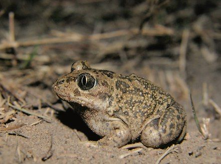
Figure 1: System Overview.

on mobile devices [38].                                       tion [42, 43, 44], however, they only use conven-
   In terms of animal voice classification, Zhang et          tional deep learning approaches such as CNN and
al. [39], Oikarinen et al. [40] study animal voice            do not make any novel improvement. In this paper,
classification using deep learning techniques. Our            we propose a multi-view CNN model and evaluation
method is different from these two works. Our stud-           results show that the proposed model outperforms
ies focus on voice classification in noisy environment        the conventional CNN.
while the voice data in [39] are collected from con-
trolled room without environmental noise. Instead             3. System Design
of classifying different animals, [40] analyses differ-
ent call types of marmoset monkeys such as Trill,             3.1. System Overview
Twitter, Phee and Chatter. Moreover, we imple-                   As shown in Figure 1, our proposed framework
ment the proposed system on a testbed and evalu-              consists of two parts: WASN and server. In the
ate its performance in real world environment. In             WASN, the wireless nodes will detect and record an-
another work [41], Stavros Ntalampiras used trans-            imal voices and then perform local processing which
fer learning to improve the accuracy of bird clas-            include silence removal, segmentation and FFT. We
sification by exploiting music genres. Their result           process signal in-situ before uploading because of
show that the transfer learning scheme can improve            the high sampling frequency of audio signal and en-
classification accuracy by 11.2%. Although the goal           ergy inefficiency of wireless communication [45, 15].
of this work and our study is to improve the recog-           The spectrum signal obtained from FFT can save
nition accuracy with deep learning technology, the            half spaces since FFT is symmetric. On the server
methodologies are different. Our approach analy-              side, the spectrum signal will be fed into a deep
ses the inherent features of audio signal and pro-            neural network to obtain the species of the animal.
pose a multi-view CNN model to improve the ac-                The classification results can be used by biologists
curacy. Instead of looking at the bird audio sig-             to analyze the density, distribution and behavior of
nals alone, Stavros Ntalampiras proposed to statis-           animals.
tically analyse audio signals using their similarities           Wireless sensors are usually resource-poor rela-
with music genres. Their method, however, is only             tive to server, and not able to run computationally
effective for a limited number of bird species be-            expensive algorithms such as deep learning mod-
cause they need to perform feature transformation             els. Therefore, we assume all the wireless sensors
again when a new bird species comes in. In compar-            can connect to a server via wireless communication
ison, our approach is applicable for a large number           technologies, such as ZigBee, Wi-Fi, and LoRa [46].
of bird species. A number of studies also apply               However, there may be network failure, server fail-
deep learning technologies in bird voice classifica-          ure, power failure, or other disruption makes offload
                                                          4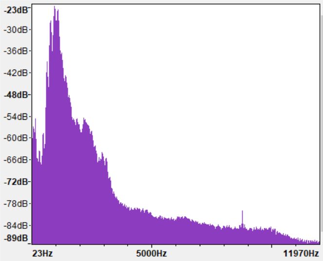
impossible. While such failures will hopefully be                 0.01
                                                                             Silence

rare, they cannot be ignored in a cloud-based sys-                  0

tem. In this case, the node can transmit the data
                                                                 -0.01
to the gateway or a nearby server which are usually                      0             0.5       1    1.5    2     2.5    3    3.5
                                                                                                                              105
resource-rich and capable of running deep learning                0.01
                                                                               Silence removed

models. Alternatively, the classification can be per-               0
formed in the node to recognize only a few species,
                                                                 -0.01
pre-defined by the user. When offloading becomes                         0             1         2     3     4      5     6     7
                                                                                                                              104
possible again, the system can revert to recognizing
its full range of species.                                                                   Figure 2: Silence removal.
   In the following parts, we will describe the design
details of each component.
                                                             is chosen to balance the trade-off between classifica-
                                                             tion accuracy and latency as discussed in Section 4.
3.2. Local Processing
                                                             The overlap in sliding window is used to capture
  Silence Removal. The collected audio signal                changes or transitions around the window limits.
usually contains a large amount of silent signal             Then we perform FFT on each segment to calcu-
when this is no animal present. Therefore, we apply          late spectrum energy (i.e. the magnitude of the
a simple silence removal method on the raw signal            FFT coefficients). As an example, Figure 3 shows
to delete not-of-interest area. The procedure is ex-         the sound in time and frequency domain of two dif-
plained in Algorithm 1. We first calculate the root          ferent frog species: Cultripes and Litoria Caerulea.
mean square (RMS) of each window which contains              It is conspicuous that they have different spectrum
1s samples and then compare it with a pre-defined            distributions. The graphs are plotted by audio sig-
threshold learned from the environment. The win-             nal analysis software Audacity.
dows of samples whose RMS above the threshold
will be kept. The threshold is determined by ex-             3.3. Multi-view Convolutional Neural Networks
haustive search. To be specific, we increase the
threshold from 0 to 0.5 with an increment of 0.01,              We propose a deep learning framework in order
then choose the one that can achieve the best per-           to automatically learn the latent and high-level fea-
formance (0.03 in this paper).                               tures from the processed audio signals for better
                                                             classification performance. Among deep learning
                                                             algorithms, CNN is widely used to discover the
Algorithm 1 Silence Removal
                                                             latent spatial information in applications such as
 1:   Input: Audio Segment Si=1:N ∈ R > 1, where             image recognition [47], ubiquitous [48], and object
      N is the total number of segments and ρ is the         searching [49], due to their salient features such
      threshold                                              as regularized structure, good spatial locality and
 2:   for i = 1 : N do                                       translation invariance. CNN applies a convolution
 3:      if RMS (Si ) < ρ then                               operation to the input, passing the result to the
 4:          Remove (Si )                                    next layer. Specifically, CNN captures the distinc-
 5:      end if                                              tive dependencies among the patterns associated to
 6:   end for                                                different audio categories. However, one drawback
                                                             of the standard CNN structure is that the filter
   Figure 2 shows an example of silence removal on           length of the convolution operation is fixed. As
an animal voice recording. We can see that it can            a result, the convolutional filter can only discover
effectively remove the silent periods and detect the         the spatial features with the fixed filter range. For
present of animals.                                          example, CNN may explore the short-term feature
   Segmentation and FFT. After silence removal,              but fail to capture the middle- and long-term fea-
we obtain audio signals containing animal vocaliza-          tures.
tion only. The audio signal is segmented into con-              To address the mentioned challenge, we propose
secutive sliding windows with 50% overlap. Ham-              a multi-view CNN framework which applies three
ming window is used in this paper to avoid spectral          different filter length to extract the short-, middle-
leakage. Each window contains 214 samples which              , and long-term features in parallel. As shown in
                                                         5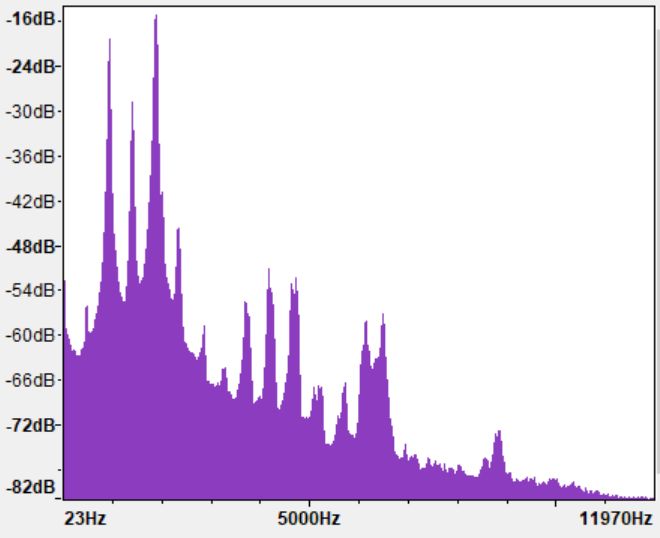
(a) Cultripes (b) Cultripes: time domain (c) Cultripes: spectrum
(d) Litoria Caerulea (e) Litoria Caerulea: time do- (f) Litoria Caerulea: spectrum
main
Figure 3: Audio signal of two species of frog.
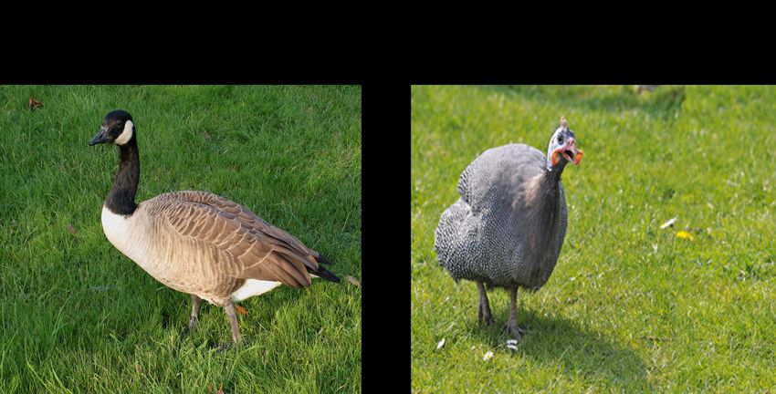
Figure 4: Multi-view CNN workflow.The audio signal is feed into three views for short-term, middle-term, and long-term
spatial dependencies learning. Convh k denotes the k-th convolutional operation in the h-th view. The learned features from the
multi-view structure are processed by the max pooling layer for dimension reduction, which are followed by the fully-connected
layer, softmax layer, and at last predict the animal species as output.
Figure 4, the proposed framework regards the pro- from the multi-view pipe are stacked together and
cessed audio signals as input and feed into three then through the max pooling operation for dimen-
views at the same time. Each view contains three sion reduction. Afterward, a fully-connected layer,
convolutional layers. Convhk denotes the k-th con- a softmax layer and the output layer work as a
volutional operation in the h-th view. The convo- classifier to predict the audio label. The proposed
lutional layer contains a set of filters to convolve multi-view CNN has several key differences from
the audio data followed by the nonlinear transfor- the inception module [50] although the ideas are
mation to extract the geographical features. The similar. First, [50] has a 1 × 1 convolutional filter
filter length keeps invariant in the same view while in the module in order to prevent the information
varies in different views. The extracted features corruption brought by inter-channel convolutions.
6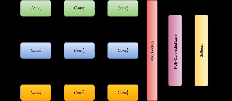
The proposed multi-view CNN does not has this                tivation. For each sample, the corresponding label
component. This is because in our case the input             information is presented by one-hot label y ∈ RH
data are naturally formed as a vector which repre-           where H denotes the category number of acoustic
sents the spectral information of the acoustic sig-          signals. The error between the predicted results
nals. Moreover, [50] adds an alternative parallel            and the ground truth is evaluated by cross-entropy
pooling path in the middle layer to acquire addi-
                                                                                       H
tional beneficial effect. However, we believe this                                     X
may cause information loss and only perform the                             loss = −          yh log(ph )
                                                                                       h=1
pooling operation after the concentration of the re-
sults of various views.                                      where ph denotes the predicted probability of ob-
   Suppose the input audio data E has shape [M, L]           servation of an object belonging to category h. The
with depth as 1. The chosen three convolutional              calculated error is optimized by the AdamOpti-
filters with size in short-, middle-, and long-term          mizer algorithm [51]. To minimize the possibility
views are [M, 10], [M, 15], [M, 20], respectively.           of overfitting, we adopt the dropout strategy and
The stride sizes keep [1, 1] for all the convolutional       set the drop rate to 80%.
layers. The stride denotes the x-movements and y-
movements distance of the filters. Since the audio
signals are arranged as 1-dimension data, we set             4. Evaluation
M = 1. Same shape zero padding is used, which
keeps the sample shape constant during the the               4.1. Goals, Metrics, and Methodology
convolution calculation. In the convolutional op-               In this section, we evaluate the performance of
eration, the feature maps from the input layer are           the proposed system based on two real datasets.
convolved with the learnable filters and fed to the          The goals of the evaluation are twofold: 1) eval-
activation function to generate the output feature           uate the performance of the proposed system un-
map. For a specific convolutional area (also called          der different settings; 2) compare the proposed
perceptive area) x which has the same shape as the           system with previous animal vocalization system.
filter, the convolutional operation can be described         We use two datasets collected from real-world for
as                       XX                                  evaluation. The first dataset contains audio sig-
              x0 = tanh(        fij ∗ xij )                  nals recorded from fourteen different species of
                         i   j                               frogs. The sampling frequency for this dataset is
where x0 denotes the filtered results while fij de-          24Khz. More details about this dataset can be
notes the i-th row and the j-th column element in            found in [15]. The second dataset 1 contains audio
the trainable filter. We adopt the widely used tanh          signals recorded from different species of crickets.
activation function for nonlinearity. The depth of           The data consists of twenty species of crickets, eight
input sample transfers to D through the convolu-             of which are Gryllidae and twelve of which are Tet-
tional layer and the sample shape is changed to              tigoniidae. The sampling frequency is also 24Khz.
[M, L, D]. In particular, the corresponding depth            More details about this dataset can be found in [1].
Dh = 2, 4, 8 for three convolutional layers. The fea-        For completeness, Table. 1 lists all the species we
tures learned from theP  filters are concatenated and        used in the experiments. In this paper, we use SVM
                            3
flattened to [1, M ∗ L ∗ h=1 Dh ]. The max pooling           and KNN to benchmark ASN classification because
has [1, 3] as both pooling length and strides. There-        they have been widely used in WASN classification
                                          P3
fore, the features with shape [1, M ∗L∗ h=1 Dh /3]           systems [8, 10, 11]. We evaluate the performance
after the pooling operation, which are forwarded to          of SVM and KNN by using frequency domain and
the fully-connected layer. The operation between             Mel-frequency cepstral coefficients (MFCCs), re-
the fully-connected layer and the output layer can           spectively. The parameters in SVM and KNN are
be represented by                                            well tuned to give highest accuracy. In addition,
                                                             we compare the accuracy of our system with a re-
             y = sof tmax(w̄E F C + b̄)                      cent work which is based on SRC [15] and con-
                                                             ventional CNN. In total, we compare our method
where F C denotes the fully-connected layer while
the w̄ and b̄ denote the corresponding weights ma-
trix and biases. The softmax function is used for ac-          1 http://alumni.cs.ucr.edu/   yhao/animalsoundfingerprint.html

                                                         7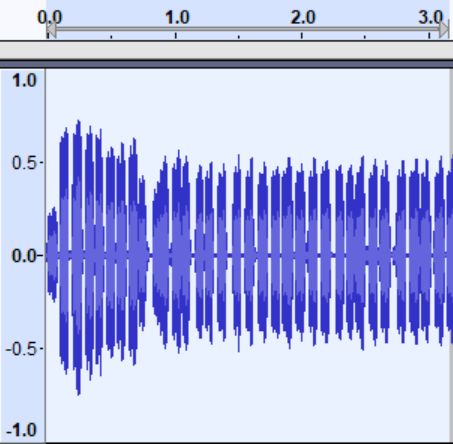
Table 1: Species used in the experiments.
Frog dataset Cricket dataset (1 belongs to Gryllidae, 2 belongs to Tettigoniidae)
Cyclorana Cryptotis Cyclorana Cultripes Acheta1 Aglaothorax2
Limnodynastes Convexiusculus Litoria Caerulea Allonemobius1 Amblycorypha2
Litoria Inermis Litoria Nasuta Anaxipha1 Anaulacomera2
1
Litoria Pallida Litoria Rubella Anurogryllus Arethaea2
Litoria Tornieri Notaden Melanoscaphus Cyrtoxipha1 Atlanticus2
Ranidella Bilingua Ranidella Deserticola Eunemobius1 Belocephalus2
Uperoleia Lithomoda Bufo Marinus Gryllus1 Borinquenula2
Hapithus1 Bucrates2
Capnobotes2 Caribophyllum2
Ceraia2 Conocephalus2
100 100 100
80 80
95
Accuracy(%)
Accuracy(%)
Accuracy(%)
60 60
90
211 window size
40 40
212 window size
213 window size
85
20 214 window size 20
215 window size
0 0 80
-10 -5 0 5 10 0 200 400 600 800 1000 0 0.1 0.2 0.3 0.4 0.5 0.6 0.7 0.8 0.9 1
SNR Number of iterations Drop out rate
(a) Impact of window size. (b) Impact of iterations. (c) Impact of dropout rate.
100 100
Our method
100
CNN
SRC
SVM-spectrum
80 KNN-spectrum 80
90
Accuracy(%)
Accuracy(%)
Accuracy(%)
60 60
80
40 40
Our method
CNN
70 SRC
20 20 SVM-MFCC
SVM-spectrum
KNN-MFCC
KNN-spectrum
60 0 0
0 1 2 3 4 5 0 20 40 60 80 100 -10 -5 0 5 10
Learning rate 10-3 Training data proportion (%) SNR
(d) Impact of learning rate. (e) Impact of training dataset. (f) Comparison with other methods.
Figure 5: Evaluation results of frog dataset.
with six classifiers: CNN, SRC, SVM-MFCC, SVM- noise to the original audio data. In this paper, we
spectrum, KNN-MFCC and KNN-spectrum. For focus on the following four metrics: accuracy, preci-
each classifier, we perform 10-fold cross-validation sion, recall and F1-score. We plot the results of the
on the collected dataset. In the original dataset, the average values and stand deviation obtained from
data only contain little environment noise. There- 10 folds cross-validation.
fore, to demonstrate the robustness of the proposed
framework, we add different scales of environmen- 4.2. Performance of Frog Dataset
tal noise to create different SNRs. This is used to 4.2.1. Impact of parameters
simulate the real environment because the recorded We first evaluate the impact of important pa-
animal voices are usually deteriorated by environ- rameters in our system. On the node’s side, the
mental noise in real WASN. In the evaluation, it is important parameters include window size of seg-
done by adding different scales of random Gaussian ment. On the server’s side, the important parame-
8Table 2: Performance of different methods on frog dataset (SNR=-6dB).
Our method CNN SRC SVM-MFCC SVM-Spectrum KNN-MFCC KNN-Spectrum
Accuracy 94.7% 82.7% 53.4% 24.4% 40.5% 20.1% 26.4%
Precision 93.1% 81.6% 54.2% 25.9% 43.5% 19.9% 25.1%
Recall 94.3% 82.4% 53.7% 24.7% 41.2% 21.5% 27.1%
F1-score 92.9% 81.2 52.1% 25.1% 39.6% 20.7% 25.7%
Figure 5(b) shows the accuracy along with dif-
ferent training iterations. We can see that the pro-
posed method converges to its highest accuracy in
less than 200 iterations. The results show that
the proposed framework can finish training quickly.
Figure 5(c) plots the accuracy of various dropout
rates. We can observe that the accuracy fluctu-
ates first and then becomes stable after the dropout
rate is greater than 0.8. Therefore, we set the de-
fault dropout rate to be 0.8. Moreover, we can infer
from Figure 5(c) that our model is not very sensi-
tive to the dropout rate. This is because the Frog
dataset matches well with the proposed multi-view
CNN, as a result, the convergence suffers less from
overfitting which can be demonstrated by the good
Figure 6: Confusion matrix of frog dataset.
convergence property as shown in Figure 5(b). Fig-
ure 5(d) shows the accuracy under different learn-
ing rates. We can see that it achieves the high-
ters include the number of iterations in training, the est accuracy when the learning rate is 0.5 × 10⁻³
dropout rate and learning rate in CNN, the size of and 1 × 10⁻³ . Correspondingly, we choose 0.001
training dataset. Dropout is a technique where ran- to reduce the training time because the smaller
domly selected neurons are ignored during training. the learning rate is, the slower the training pro-
For example, the dropout rate of 80% means that cess is. From Figure 5(d), we can observe that the
we randomly select 20% of the neurons and drop performance varies dramatically with the increas-
them (force the values of them as 0). The dropout ing of learning rate. One possible reason for this
strategy is widely used to enhance the generaliza- is that the gradient surface of our loss function is
tion of a machine learning model and prevent over- not smooth and very sensitive to the learning rate.
fitting. The learning rate is a hyper-parameter that The optimiser is easy to step over the local optima
controls how much we are adjusting the weights of while the learning rate is larger than a threshold.
the neuron network with respect to the loss gradi- Next, we evaluate the accuracy of the proposed
ent. system under different sizes of training dataset. In
To evaluate the impact of window size, we vary this experiment, we use different proportions of the
the window size from 211 to 215 samples and calcu- whole dataset for training, and use the left dataset
late the accuracy of our scheme. From the results in for testing. The proportion increases from 10% to
Figure 5(a), we can see that there is a performance 90% with an increment of 10%. For example, the
gain when we increase the window size and the im- proportion of 10% means we use 10% of the dataset
provement reduces after 214 samples. Although we for training, and use the left dataset for testing.
can achieve higher accuracy with more samples, the For comparison purpose, we also calculate the ac-
resource consumption of FFT operation which runs curacy of CNN, SRC, SVM and KNN. From the
on the wireless sensor node also increases. There- results in Figure 5(e), we can see that our method
fore, we choose to use 214 window size to balance continuously achieves the highest accuracy, and the
the trade-off between accuracy and resource con- accuracy becomes relatively stable after 60% of the
sumption. dataset is used for training. We also notice that
9100 100 100
80 80
95
Accuracy(%)
Accuracy(%)
Accuracy(%)
60 60
90
40 211 window size 40
12
2 window size
13
2 window size 85
20 214 window size 20
215 window size
0 0 80
-10 -5 0 5 10 0 200 400 600 800 1000 0 0.1 0.2 0.3 0.4 0.5 0.6 0.7 0.8 0.9 1
SNR Number of iterations Drop out rate
(a) Impact of window size. (b) Impact of iterations. (c) Impact of dropout rate.
100 100
Our method
CNN
SRC
SVM-spectrum
80
90 KNN-spectrum
Accuracy(%)
Accuracy(%)
60
80
40
70
20
60 0
0 1 2 3 4 5 0 20 40 60 80 100
Learning rate 10-3 Training data proportion (%)
(d) Impact of learning rate. (e) Impact of training dataset.
Figure 7: Evaluation results of cricket dataset.
the improvement of our method from 10% to 90% that different frog species are not distinguishable in
is remarkable. More specifically, when the propor- MFCC feature space. The results also explains why
tion of the training dataset increases from 10% to MFCC-based methods usually requires other care-
90%, the accuracy improvement of our method is fully selected features [28]. We find that when the
40.1% while the improvement of CNN, SRC, SVM animal voice is overwhelmed by environmental noise
and KNN are 34.7%, 29.3%, 26.7% and 22.4%, re- (low SNR), the accuracy of our system is signifi-
spectively. In this experiment, we do not test SVM- cantly higher than the other methods. For example,
MFCC and KNN-MFCC because their accuracy is when SN R = −6dB, the accuracy of our method
poor as will be shown later. is 12% higher than CNN, 41% higher than SRC,
70% higher than SVM-MFCC, 53.9% higher than
4.2.2. Comparison With Other Methods SVM-spectrum, 74.3% higher than KNN-MFCC,
We now compare the performance of proposed and 68% higher than KNN-spectrum. The robust-
scheme with previous approaches. As mentioned ness to noise makes the proposed system suitable
above, we compare the accuracy of the proposed for real deployment in noisy environments. More-
system with conventional CNN, SRC, SVM-MFCC, over, the results also indicate that our system needs
SVM-spectrum, KNN-MFCC and KNN-spectrum. less sensors to cover a certain area because our sys-
The MFCC of each window is calculated by trans- tem can classify low SNR signals which are usually
forming the power spectrum of each window into collected from longer distance.
the logarithmic mel-frequency spectrum. We cal-
culate the accuracy of different methods under dif- To take a closer look at the result, we summarize
ferent SNRs by adding different scales of environ- the results of different methods in Table 2 and plot
mental noise. confusion matrix in Figure 6 when SNR is -6dB. We
As we can see from Figure 5(f), SVM-MFCC and can see that each class can achieve high accuracy
KNN-MFCC performs the worst which suggests and the overall average accuracy is 94.7%.
10Table 3: Performance of different methods on cricket dataset (SNR=-6dB).
Our method CNN SRC SVM-MFCC SVM-Spectrum KNN-MFCC KNN-Spectrum
Accuracy 86.4% 76.6% 42.4% 22.1% 36.8% 19.4% 28.5%
Precision 86.9% 76.2% 42.5% 23.6% 36.3% 18.2% 28.6%
Recall 85.1% 75.3% 41.2% 22.7% 37.3% 19.9% 29.8%
F1-score 86.1% 74.6% 41.7% 21.8% 38.1% 19.5% 29.5%
100 of twenty species of insects, eight of which are
Gryllidae and twelve of which are Tettigoniidae.
80 Thus, we can treat the problem as either a two-
class genus level problem, or twenty-class species
Accuracy(%)
60
level problem. We first treat the classification as a
Our method
two-class level problem and calcualte the accuracy
40 CNN
SRC of different methods under different SNRs. From
SVM-MFCC
20 SVM-spectrum the results in Figure 8(a), we can see that our
KNN-MFCC
KNN-spectrum method, SRC, SVM-spectrum and KNN-spectrum
0
-10 -5 0 5 10
can achieve high accuracy. However, our method
SNR still outperforms all the other classifiers. There-
(a) Two-class classification. after, we treat the classification as a twenty-class
species level problem and plot the accuracy of dif-
100
ferent methods in Figure 8(a). We can see that
the proposed method significantly outperforms the
80 other methods when SNR is low. Table 3 summa-
rizes the results of each method in detail. The
Accuracy(%)
60 results above demonstrate the advantage of our
method in classifying more species in noisy envi-
40
Our method
ronment.
CNN
SRC
20 SVM-MFCC
SVM-spectrum
KNN-MFCC 5. Case Study on Testbed
KNN-spectrum
0
-10 -5 0 5 10 To validate the feasibility of the proposed frame-
SNR
work in real environment, we implement the sys-
(b) Twenty-class classification.
tem on an outdoor ASN testbed which is located in
Brisbane, Australia. As shown in Figure 9(a), the
Figure 8: 2 class classification vs 20 class classification.
testbed is composed of five nodes which are config-
ured as Ad-hoc mode with a star network topology.
4.3. Performance of Cricket Dataset Its task is to evaluate the system’s capability of
recognizing bird vocalization in real world environ-
Similar to Frog dataset, we also evaluate the im- ment.
pact of window size, the number of iterations, the
dropout rate and learning rate in CNN, and the size Table 4: Power Consumption.
of training dataset using Cricket dataset. The pro-
cedures are the same as above and the results are Module Consumption (W)
shown in Figure 8. We can see that it shows simi- CPU 2.05
lar patterns as Frog dataset which suggests that the CPU + microphone 2.1
proposed framework is robust to different species. CPU + Wifi (idle) 2.45
In terms of the dropout rate and learning rate, the CPU + Wifi (Rx) 2.67
optimal values for dropout rate and learning rate CPU + Wifi (Tx) 2.78
are 0.7 and 0.0005 which is slightly different from
that of Frog dataset. The hardware platform used in the testbed is
As mentioned in [1], the cricket dataset consists based on a Pandaboard ES with an 1.2Ghz OMAP
11(a) Network topology (b) Bird species
Figure 9: Testbed.
4460, 1GB Ram and 4GB SD-card. Additionally, Table 5: Computation time of local processing.
Pandaboard includes an 802.11 interface for wire-
less connection. Microphones are connected to the Silence Removal FFT
Pandaboard via USB port to record bird voice with Time (ms) 20.38 ± 2.04 15.33 ± 0.63
24Khz sampling rate. All the nodes are connected
via the local Wi-Fi network. The data collected
from Node 2, 3, 4 and 5 will be first transferred to Second, we apply a Butterworth high pass filter
Node 1. Then, all the data will be uploaded from with 200Hz cut-off frequency to filter out unwanted
Node 1 to the local server. The acoustic date from noise. This is because most of the wind audio en-
different nodes are classified separately in the sys- ergy lies in the frequency band below 200Hz, while
tem. most of the vocalization energy of the birds is in
In the testbed, each node is powered by a the frequency band higher than 200Hz.
rechargeable battery (12V, 7.2Ah), and an optional After implementing the proposed framework on
solar panel (5W, 12V). The power consumption of the testbed, we calculate the computation time on
each module is given in Table 4. Compared to the node’s side and classification accuracy on the
SolarStore testbed [52] which consumes 10W (low server’s side. On the node’s side, we find that the
load) and 15W (high load) energy, our testbed is ap- node in our testbed can process all the captured
proximately 3.5 to 5.4 times more energy efficient. acoustic data in real time. From Table 6, we can
Without solar panel, a node in our ASN testbed see the silence removal and FFT take 20.38 ms and
will run continuously for more than 31 hours, which 15.33 ms, respectively.
is significantly longer than the previous platforms In this study, we choose two common bird species
such as ENSBox [53]. We find that if a solar panel in the area of interest: Anseriformes and Galli-
is exposed to direct sunlight for 8 hours per day, the formes (Figure 9(b)). Our goal is to classify the
node can maintain a 50% duty cycle at 85% solar voice into three classes: Anseriformes, Galliformes
charge efficiency. and others. The testbed runs for 30 days and the
The nodes use Network Time Protocol (NTP) for data is labeled manually. Table 6 lists the re-
time synchronization. We use one node as the NTP sults of different methods for classification in the
server, and the other nodes as the NTP clients. The server. We find that the proposed system achieve
NTP clients send request for time synchronization 90.3% classification accuracy which outperforms
every 10 seconds. The accuracy of time synchro- other methods significantly. The results in turn
nization is about 25 ms, which is good enough for suggest that the proposed framework is robust to
our distributed real-time system because the length environmental noise and can achieve high classifica-
of each testing signal segment is 400ms. tion accuracy in real-world WASN. We also notice
During deployment, we found that the recorded that the results of the case study is slightly lower
voice is deteriorated by wind. To solve this prob- than the simulation results in Section 4. This is
lem, we take two measures. First, we install because the public dataset are collected in a con-
foam and fur windscreen around each microphone. trolled manner and the signals are well trimmed and
12Table 6: Performance on testbed.
Our system CNN SRC SVM-Spectrum KNN-Spectrum
Accuracy 90.3% 84.4% 72.3% 65.7% 68.8%
Precision 91.2% 82.1% 72.6% 66.4% 69.2%
Recall 89.4% 84.6% 70.9% 65.6% 67.1%
F1-score 91.1% 83.7% 71.8% 66.4% 70.5%
processed. However, the data we used in our case [5] D. J. Nowak, J. E. Pasek, R. A. Sequeira, D. E. Crane,
study are collected in a totally automatic manner. V. C. Mastro, Potential effect of anoplophora glabripen-
nis (coleoptera: Cerambycidae) on urban trees in the
united states, Journal of economic entomology 94 (1)
6. Conclusion (2001) 116–122.
[6] S. E. Anderson, A. S. Dave, D. Margoliash, Template-
In this paper, we design and implement a CNN- based automatic recognition of birdsong syllables from
continuous recordings, The Journal of the Acoustical
based acoustic classification system for WASN. To Society of America 100 (2) (1996) 1209–1219.
improve the accuracy in noisy environment, we pro- [7] J. A. Kogan, D. Margoliash, Automated recognition of
pose a multi-view CNN framework which contains bird song elements from continuous recordings using dy-
namic time warping and hidden markov models: A com-
three convolution operation with three different fil-
parative study, The Journal of the Acoustical Society
ter length in parallel in order to extract the short- of America 103 (4) (1998) 2185–2196.
, middle-, and long-term information at the same [8] S. Fagerlund, Bird species recognition using support
time. Extensive evaluations on two real datasets vector machines, EURASIP Journal on Applied Signal
Processing 2007 (1) (2007) 64–64.
show that the proposed system significantly outper- [9] G. Guo, S. Z. Li, Content-based audio classification
forms previous methods. To demonstrate the per- and retrieval by support vector machines, IEEE trans-
formance of the proposed system in real world envi- actions on Neural Networks 14 (1) (2003) 209–215.
ronment, we conduct a case study by implementing [10] C.-J. Huang, Y.-J. Yang, D.-X. Yang, Y.-J. Chen, Frog
classification using machine learning techniques, Expert
our system in a public testbed. The results show Systems with Applications 36 (2) (2009) 3737–3743.
that our system works well and can achieve high ac- [11] M. A. Acevedo, C. J. Corrada-Bravo, H. Corrada-
curacy in real deployments. In our future work, we Bravo, L. J. Villanueva-Rivera, T. M. Aide, Automated
will deploy the proposed framework in wider area classification of bird and amphibian calls using machine
learning: A comparison of methods, Ecological Infor-
and evaluate its performance in different environ- matics 4 (4) (2009) 206–214.
ments. [12] R. Banerjee, M. Mobashir, S. D. Bit, Partial dct-
based energy efficient compression algorithm for wire-
less multimedia sensor network, in: Proceedings of the
Acknowledgement 2014 IEEE International Conference on Electronics,
Computing and Communication Technologies (IEEE
The work described in this paper was fully sup- CONECCT), IEEE, 2014, pp. 1–6.
ported by a grant from City University of Hong [13] I. Dutta, R. Banerjee, S. D. Bit, Energy efficient au-
dio compression scheme based on red black wavelet lift-
Kong (Project No.7200642) ing for wireless multimedia sensor network, in: Pro-
ceedings of the 2013 International Conference on Ad-
vances in Computing, Communications and Informatics
References (ICACCI), IEEE, 2013, pp. 1070–1075.
[14] J. J. Diaz, E. F. Nakamura, H. C. Yehia, J. Salles, A. A.
[1] Y. Hao, B. Campana, E. Keogh, Monitoring and mining
Loureiro, On the use of compressive sensing for the re-
animal sounds in visual space, Journal of insect behav-
construction of anuran sounds in a wireless sensor net-
ior 26 (4) (2013) 466–493.
work, in: Proceedings of the 2012 IEEE International
[2] J. Luque, D. F. Larios, E. Personal, J. Barbancho,
Conference on Green Computing and Communications
C. León, Evaluation of mpeg-7-based audio descriptors
(GreenCom), IEEE, 2012, pp. 394–399.
for animal voice recognition over wireless acoustic sen-
[15] B. Wei, M. Yang, Y. Shen, R. Rana, C. T. Chou,
sor networks, Sensors 16 (5) (2016) 717.
W. Hu, Real-time classification via sparse representa-
[3] I. F. Akyildiz, D. Pompili, T. Melodia, Underwater
tion in acoustic sensor networks, in: Proceedings of the
acoustic sensor networks: research challenges, Ad hoc
11th ACM Conference on Embedded Networked Sensor
networks 3 (3) (2005) 257–279.
Systems (Sensys), ACM, 2013, p. 21.
[4] W. Hu, N. Bulusu, C. T. Chou, S. Jha, A. Taylor, V. N.
[16] Y. Shen, W. Hu, M. Yang, B. Wei, S. Lucey, C. T.
Tran, Design and evaluation of a hybrid sensor network
Chou, Face recognition on smartphones via optimised
for cane toad monitoring, ACM Transactions on Sensor
sparse representation classification, in: Proceedings of
Networks (TOSN) 5 (1) (2009) 4.
13the 13th international symposium on Information pro- works with convolutional attentions for multi-modality
cessing in sensor networks, IEEE Press, 2014, pp. 237– activity modeling, Proceedings of the 2018 Interna-
248. tional Joint Conference on Neural Networks (IJCNN-
[17] W. Xu, Y. Shen, N. Bergmann, W. Hu, Sensor-assisted 18) (2018).
face recognition system on smart glass via multi-view [32] C. Luo, X. Feng, J. Chen, J. Li, W. Xu, W. Li, L. Zhang,
sparse representation classification, in: Proceedings of Z. Tari, A. Y. Zomaya, Brush like a dentist: Accu-
the 2016 15th ACM/IEEE International Conference rate monitoring of toothbrushing via wrist-worn gesture
on Information Processing in Sensor Networks (IPSN), sensing, in: INFOCOM, IEEE, 2019, pp. 1234–1242.
IEEE, 2016, pp. 1–12. [33] X. Zhang, L. Yao, C. Huang, S. Wang, M. Tan, G. Long,
[18] Y. Sun, Y. Chen, X. Wang, X. Tang, Deep learning C. Wang, Multi-modality sensor data classification with
face representation by joint identification-verification, selective attention, in: Proceedings of the 27th Interna-
in: Advances in neural information processing systems, tional Joint Conference on Artificial Intelligence IJCAI-
2014, pp. 1988–1996. 18, International Joint Conferences on Artificial Intelli-
[19] G. Hinton, L. Deng, D. Yu, G. E. Dahl, A.-r. Mohamed, gence Organization, 2018, pp. 3111–3117.
N. Jaitly, A. Senior, V. Vanhoucke, P. Nguyen, T. N. [34] G. Lan, W. Xu, D. Ma, S. Khalifa, M. Hassan, W. Hu,
Sainath, et al., Deep neural networks for acoustic mod- Entrans: Leveraging kinetic energy harvesting signal for
eling in speech recognition: The shared views of four re- transportation mode detection, IEEE Transactions on
search groups, IEEE Signal processing magazine 29 (6) Intelligent Transportation Systems (2019).
(2012) 82–97. [35] W. Xu, X. Feng, J. Wang, C. Luo, J. Li, Z. Ming, En-
[20] A. Graves, A.-r. Mohamed, G. Hinton, Speech recogni- ergy harvesting-based smart transportation mode de-
tion with deep recurrent neural networks, in: Proceed- tection system via attention-based lstm, IEEE Access
ings of the 2013 ieee international conference on Acous- (2019).
tics, speech and signal processing (icassp), IEEE, 2013, [36] X. Zhang, L. Yao, S. S. Kanhere, Y. Liu, T. Gu,
pp. 6645–6649. K. Chen, Mindid: Person identification from brain
[21] R. Collobert, J. Weston, A unified architecture for nat- waves through attention-based recurrent neural net-
ural language processing: Deep neural networks with work, Proceedings of the ACM on Interactive, Mobile,
multitask learning, in: Proceedings of the 25th interna- Wearable and Ubiquitous Technologies 2 (3) (2018) 149.
tional conference on Machine learning, ACM, 2008, pp. [37] N. D. Lane, P. Georgiev, Can deep learning revolution-
160–167. ize mobile sensing?, in: Proceedings of the 16th Inter-
[22] Y. Wang, M. Huang, L. Zhao, et al., Attention-based national Workshop on Mobile Computing Systems and
lstm for aspect-level sentiment classification, in: Pro- Applications, ACM, 2015, pp. 117–122.
ceedings of the 2016 conference on empirical methods [38] N. D. Lane, S. Bhattacharya, P. Georgiev, C. Forlivesi,
in natural language processing, 2016, pp. 606–615. L. Jiao, L. Qendro, F. Kawsar, Deepx: A software accel-
[23] G. Jahns, W. Kowalczyk, K. Walter, Sound analysis to erator for low-power deep learning inference on mobile
recognize different animals, IFAC Proceedings Volumes devices, in: Proceedings of the 15th International Con-
30 (26) (1997) 169–173. ference on Information Processing in Sensor Networks,
[24] D. G. Preatoni, M. Nodari, R. Chirichella, G. Tosi, IEEE Press, 2016, p. 23.
L. A. Wauters, A. Martinoli, Identifying bats from time- [39] Y.-J. Zhang, J.-F. Huang, N. Gong, Z.-H. Ling, Y. Hu,
expanded recordings of search calls: comparing classi- Automatic detection and classification of marmoset vo-
fication methods, The Journal of wildlife management calizations using deep and recurrent neural networks,
69 (4) (2005) 1601–1614. The Journal of the Acoustical Society of America
[25] M. Hodon, P. Šarafı́n, P. Ševčı́k, Monitoring and recog- 144 (1) (2018) 478–487.
nition of bird population in protected bird territory, in: [40] T. P. Oikarinen, K. Srinivasan, O. Meisner, J. B. Hy-
2015 IEEE Symposium on Computers and Communi- man, S. Parmar, R. Desimone, R. Landman, G. Feng,
cation (ISCC), IEEE, 2015, pp. 198–203. Deep convolutional network for animal sound classifica-
[26] P. A. Eliopoulos, I. Potamitis, D. C. Kontodimas, Esti- tion and source attribution using dual audio recordings,
mation of population density of stored grain pests via bioRxiv (2018) 437004.
bioacoustic detection, Crop Protection 85 (2016) 71–78. [41] S. Ntalampiras, Bird species identification via transfer
[27] S. Ntalampiras, Automatic acoustic classification of in- learning from music genres, Ecological informatics 44
sect species based on directed acyclic graphs, The Jour- (2018) 76–81.
nal of the Acoustical Society of America 145 (6) (2019) [42] I. Potamitis, Deep learning for detection of bird vocal-
EL541–EL546. isations, arXiv preprint arXiv:1609.08408 (2016).
[28] G. Vaca-Castaño, D. Rodriguez, Using syllabic mel cep- [43] H. V. Koops, J. Van Balen, F. Wiering, A deep neu-
strum features and k-nearest neighbors to identify anu- ral network approach to the lifeclef 2014 bird task,
rans and birds species, in: 2010 IEEE workshop On CLEF2014 Working Notes 1180 (2014) 634–642.
Signal processing systems (SIPS), IEEE, 2010, pp. 466– [44] H. Goëau, H. Glotin, W.-P. Vellinga, R. Planqué,
471. A. Joly, Lifeclef bird identification task 2016: The ar-
[29] Y. Sun, H. Qi, Dynamic target classification in wireless rival of deep learning, 2016.
sensor networks, in: 2008 19th International Conference [45] K. C. Barr, K. Asanović, Energy-aware lossless data
on Pattern Recognition, IEEE, 2008, pp. 1–4. compression, ACM Transactions on Computer Systems
[30] Y. Wen, K. Zhang, Z. Li, Y. Qiao, A discriminative (TOCS) 24 (3) (2006) 250–291.
feature learning approach for deep face recognition, in: [46] W. Xu, J. Y. Kim, W. Huang, S. Kanhere, S. Jha,
European Conference on Computer Vision, Springer, W. Hu, Measurement, characterization and modeling of
2016, pp. 499–515. lora technology in multi-floor buildings, IEEE Internet
[31] K. Chen, L. Yao, X. Wang, D. Zhang, T. Gu, Z. Yu, of Things Journal (2019).
Z. Yang, Interpretable parallel recurrent neural net-
14[47] D. C. Ciresan, U. Meier, L. M. Gambardella, J. Schmid- Machine Intelligence (6) (2017) 1137–1149.
huber, Convolutional neural network committees for [50] C. Szegedy, W. Liu, Y. Jia, P. Sermanet, S. Reed,
handwritten character classification, in: Proceedings of D. Anguelov, D. Erhan, V. Vanhoucke, A. Rabinovich,
the 2011 International Conference on Document Anal- Going deeper with convolutions, in: Proceedings of the
ysis and Recognition (ICDAR), IEEE, 2011, pp. 1135– IEEE conference on computer vision and pattern recog-
1139. nition, 2015, pp. 1–9.
[48] R. Ning, C. Wang, C. Xin, J. Li, H. Wu, Deepmag: [51] D. P. Kingma, J. Ba, Adam: A method for stochastic
Sniffing mobile apps in magnetic field through deep con- optimization, arXiv preprint arXiv:1412.6980 (2014).
volutional neural networks, in: Proceedings of the 2018 [52] Y. Yang, L. Wang, D. K. Noh, H. K. Le, T. F. Ab-
IEEE International Conference on Pervasive Comput- delzaher, Solarstore: enhancing data reliability in solar-
ing and Communications (PerCom), IEEE, 2018, pp. powered storage-centric sensor networks, in: MobiSys,
1–10. ACM, 2009, pp. 333–346.
[49] S. Ren, K. He, R. Girshick, J. Sun, Faster r-cnn: to- [53] L. Girod, M. Lukac, V. Trifa, D. Estrin, The design and
wards real-time object detection with region proposal implementation of a self-calibrating distributed acoustic
networks, IEEE Transactions on Pattern Analysis & sensing platform, in: SenSys, ACM, 2006, pp. 71–84.
15You can also read