Mesoscale Structure in the Solar Wind - Frontiers
←
→
Page content transcription
If your browser does not render page correctly, please read the page content below
REVIEW
published: 25 August 2021
doi: 10.3389/fspas.2021.735034
Mesoscale Structure in the Solar Wind
N. M. Viall 1*, C. E. DeForest 2 and L. Kepko 1
1
NASA Goddard Space Flight Center, Greenbelt, MD, United States, 2Department of Space Studies, Southwest Research
Institute, Boulder, CO, United States
Structures in the solar wind result from two basic mechanisms: structures injected or
imposed directly by the Sun, and structures formed through processing en route as the
solar wind advects outward and fills the heliosphere. On the largest scales, solar structures
directly impose heliospheric structures, such as coronal holes imposing high speed
streams of solar wind. Transient solar processes can inject large-scale structure
directly into the heliosphere as well, such as coronal mass ejections. At the smallest,
kinetic scales, the solar wind plasma continually evolves, converting energy into heat, and
all structure at these scales is formed en route. “Mesoscale” structures, with scales at 1 AU
in the approximate spatial range of 5–10,000 Mm and temporal range of 10 s–7 h, lie in the
orders of magnitude gap between the two size-scale extremes. Structures of this size
regime are created through both mechanisms. Competition between the imposed and
injected structures with turbulent and other evolution leads to complex structuring and
dynamics. The goal is to understand this interplay and to determine which type of
mesoscale structures dominate the solar wind under which conditions. However, the
Edited by: mesoscale regime is also the region of observation space that is grossly under-sampled.
Marina Stepanova,
University of Santiago, Chile
The sparse in situ measurements that currently exist are only able to measure individual
Reviewed by:
instances of discrete structures, and are not capable of following their evolution or spatial
Roberto Elías Navarro, extent. Remote imaging has captured global and large scale features and their evolution,
University of Concepcion, Chile
but does not yet have the sensitivity to measure most mesoscale structures and their
Daniel Verscharen,
University College London, evolution. Similarly, simulations cannot model the global system while simultaneously
United Kingdom resolving kinetic effects. It is important to understand the source and evolution of solar wind
*Correspondence: mesoscale structures because they contain information on how the Sun forms the solar
N. M. Viall
nicholeen.m.viall@nasa.gov
wind, and constrains the physics of turbulent processes. Mesoscale structures also
comprise the ground state of space weather, continually buffeting planetary
Specialty section: magnetospheres. In this paper we describe the current understanding of the formation
This article was submitted to
and evolution mechanisms of mesoscale structures in the solar wind, their characteristics,
Space Physics,
a section of the journal implications, and future steps for research progress on this topic.
Frontiers in Astronomy and Space
Sciences Keywords: sun, heliosphere, solar wind, geospace, space weather, turbulence, solar variability, mesoscales
Received: 02 July 2021
Accepted: 10 August 2021
Published: 25 August 2021 1 INTRODUCTION
Citation:
The solar corona is comprised of a hot, ≥1 MK plasma that expands outward into the solar system,
Viall NM, DeForest CE and Kepko L
(2021) Mesoscale Structure in the
carrying magnetic field with it, and reaching flow speeds greater than the Alfvén speed. This flow is
Solar Wind. the solar wind, and defines the heliosphere. The solar wind is not laminar, but is dynamic and filled
Front. Astron. Space Sci. 8:735034. with structures on many spatial and temporal scales, from the large down through kinetic dissipation
doi: 10.3389/fspas.2021.735034 scales. The largest scales are directly imposed onto or injected into the solar wind, and include the
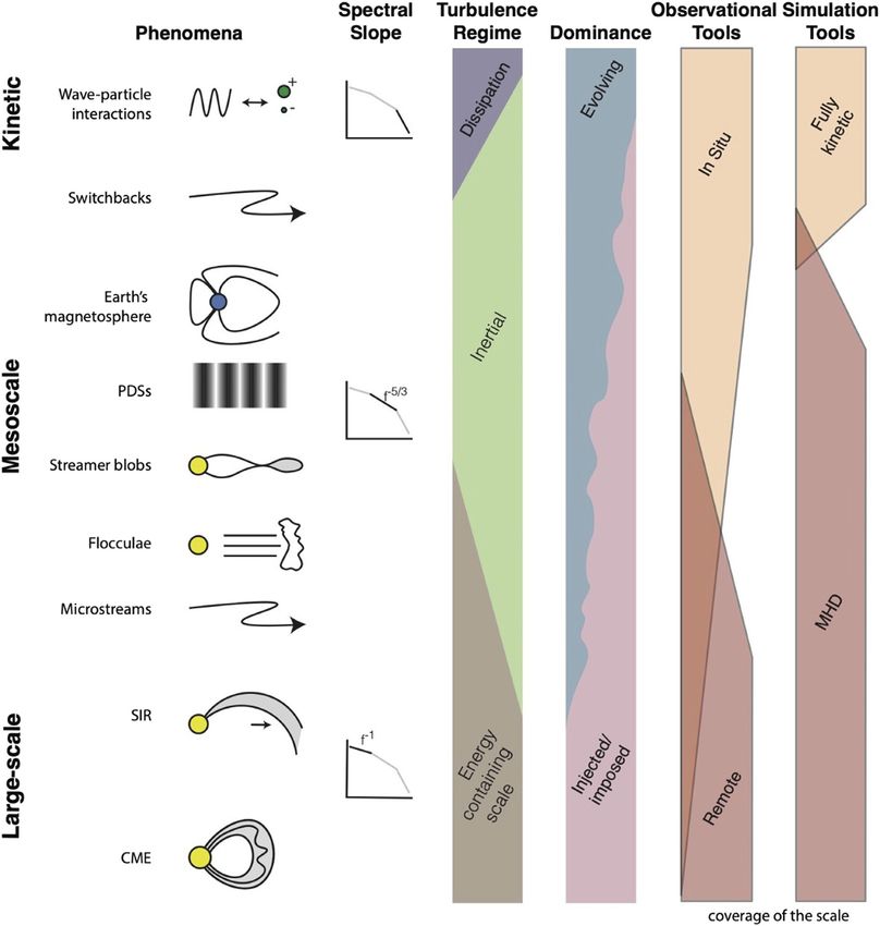
Frontiers in Astronomy and Space Sciences | www.frontiersin.org 1 August 2021 | Volume 8 | Article 735034Viall et al. Solar Wind Mesoscale Structure FIGURE 1 | The spatial scales of solar wind phenomena span from the kinetic (
Viall et al.                                                                                                          Solar Wind Mesoscale Structure

by L  Vsw p duration, while in images both spatial and temporal             both imposed/injected from the Sun as well as generated en route.
scales can be directly measured.                                             The upper end is roughly 10,000 Mm (or 7 h), based on
    In Figure 1 we show a conceptual view of the full range of               observational and theoretical evidence for mesoscale structures
scales in the solar wind, and highlight representative examples of           that were created in both ways. These sources of mesoscale
solar wind phenomena observed at the different scales. The y-axis            structure are not mutually exclusive, as structures from the
shows the range of scale sizes from large-scale to kinetic. From left        solar atmosphere will also evolve as they advect. Thus, the
to right, we provide representative cartoon examples of each scale,          complexity in this mesoscale regime is a result of the presence
example spectral slopes of the measured plasma variations, the               of both imposed/injected and evolved structures, and the
corresponding turbulence regime, whether the scales’ creation is             interplay between them. Determining the fractional amount of
dominated by injected/imposed versus evolution, the ability of               mesoscale structures formed through imposed/injected versus
current observations to measure them, and the ability of current             evolved is important for understanding both solar wind
simulations to model them.                                                   formation and turbulent evolution, and the answer is likely
    At the smallest scale lies the kinetic scale, where plasma               dependent on solar wind type and radial distance (evolution
dynamics and structure are dictated by the motion of                         time) from the Sun.
individual particles. The transition between the kinetic and the                Mesoscale solar wind structures are important to study for at
mesoscale is generally considered to be related to the ion inertial          least three reasons. First, like the solar wind, the Sun is also
length, di, or the ion gyroradius. At 1 AU, the observed break in            dynamic and filled with structures of many scales. Many of the
the spectra of magnetic field fluctuations from the inertial range             spatial structures are imposed directly onto the heliosphere, and
to the dissipation scales typically is observed to occur at advected         many of the transient dynamics are injected directly into the solar
time scales of several seconds (Leamon et al., 1999), or                     wind as it is formed. Thus, the solar wind and its structures
equivalently on spatial scales on the order of hundreds of km                contain imprints of the physical processes that heat the corona
through a few Mm via the Taylor hypothesis (that spatial crossing            and that release and accelerate the solar wind (Viall and
time dominates temporal behavior of the solar wind as measured               Borovsky, 2020). In particular, the traditional bimodal solar
in situ). This scale is close to the proton cyclotron frequency              wind classification by speed overly simplifies the inherent
(Verscharen et al., 2019) though multiple mechanisms have been               nature and mesoscale structure of the solar wind.
suggested to explain this spectral break (Leamon et al., 1999).              Furthermore, the bimodal classification does not account for
Note also that the Taylor hypothesis has limitations in the context          solar wind observed to be of other “types” with distinct
of turbulence (Treumann et al., 2019; Bourouaine and Perez,                  properties (Roberts et al., 2020a), e.g., slow wind that is highly
2020; Perez et al., 2021). At these small scales, all of the structure       Alfvénic (Roberts et al., 1987; D’Amicis and Bruno, 2015). Rather
and dynamics are created as a result of processing and evolution             than only two types of solar wind, solar wind formation can occur
en route to 1 AU. Any injected or imposed structure from the                 via many different pathways, or combinations of physical
corona begins to evolve on timescales as rapid as the wave-                  mechanisms and source locations (Viall and Borovsky, 2020),
particle interaction time scale (Bruno and Carbone, 2013);                   each of which injects and imposes different structures with
structural evolution on small scales has been observed both in-              unique properties into the solar wind. Some pathways to solar
situ (Elliott et al., 2016) and (on larger scales) remotely (DeForest        wind formation result in solar wind plasma with properties and
et al., 2015).                                                               mesoscale structures that cannot be interpreted with the simple
    The largest scale solar wind structures are all imposed/injected         bimodal classification.
from the Sun. For example, the traditional solar wind separation                A key aspect of the new framework that allows for many
by speed into “fast” and “slow” wind (Neugebauer and Snyder,                 pathways to solar wind formation is that it considers the time
1962; Neugebauer and Snyder, 1966; McComas et al., 1998), are                history of the solar plasma as it becomes the solar wind. This oft-
empirically associated with and imposed by the large scale solar             ignored time history of solar wind formation imparts unique,
structures coronal holes and coronal streamers, respectively. Co-            observable imprints of the physical regime and processes that
rotating interaction regions (CIR) and stream interaction regions            dominate each step; mesoscale structures can be one of the
(SIR) form due to adjacent faster and slower wind regions in                 results. Observations of collisionality (Kasper et al., 2008;
combination with solar rotation, producing compression regions               Kasper et al., 2017) and composition (Zurbuchen et al., 2002)
where the fast wind catches up with the slow, and rarefaction                are also examples where the solar wind exhibits a continuum of
regions behind (Gosling and Pizzo, 1999). This is an example of              states rather than bimodality, and are examples where the time
directly imposed structures that have been observed in white light           history of the plasma likely influences the resulting solar wind
and tracked to 1 AU using combined STEREO SECCHI                             characteristics. The three steps of solar wind formation time
Heliospheric imager data and L1 in situ observations                         history are source, release, and acceleration. The first step is the
(Rouillard et al., 2009; Rouillard et al., 2010a; Rouillard et al.,          source of the plasma–i.e., whether it originates from a coronal
2010b), and evidence of them survives out to 10 AU (Richardson,              hole (CH), which are tenuous and cooler, an active region (AR),
2018).                                                                       which are dense and hot, or from the quiet sun (QS), which are of
    The transition from the large scale to the mesoscale range is            medium temperatures and densities. Separating the solar wind
more ambiguous than the transition from small scale to                       source into these three types of locations in the corona, which
mesoscales. For the purposes of this paper, we define the                     themselves are associated with different solar magnetic field
mesoscales to be the scales at 1 AU at which structures can be               configurations and plasma conditions, is essentially an

Frontiers in Astronomy and Space Sciences | www.frontiersin.org          3                                    August 2021 | Volume 8 | Article 735034
Viall et al. Solar Wind Mesoscale Structure
empirical proxy for coronal heating (Viall et al., 2021). The 1993; Crooker et al., 1996b), predating observations that were
second step is the release of plasma–whether the plasma is on capable of conclusively and routinely differentiating between
open magnetic field lines, with one footpoint rooted in the Sun possible sources. Some fraction of the injected or imposed
and the other already open to the heliosphere, or whether the structures provide the energy for the turbulent cascade, or
plasma is on closed magnetic field lines, with both magnetic otherwise evolve as they advect, which we will describe in
footpoints rooted in the Sun, requiring reconnection for the Section 3. In this section we focus on identifiable structures
plasma to be released into solar wind. The third step is plasma that are unambiguously of solar origin.
acceleration, a process that continues through the high corona. There exist two main observational methods for
All three steps can occur through a single physical process, such unambiguously identifying structures that were injected/
as turbulence; in such cases, the coronal heating mechanism, solar imposed from the Sun. The first and most direct method is
wind release, and solar wind acceleration all result from the same through remote imaging. This is typically done in white light,
process (Cranmer et al., 2017). However, whenever the second which is sensitive to electron density and location relative to the
step is reconnection, then steps one and three are necessarily Thomson Surface (Vourlidas and Howard, 2006; Howard and
separate processes because they occur in different physical DeForest, 2012), or extreme ultraviolet (EUV) emission, which is
regimes, thus leaving distinct plasma observables and sensitive to electron density squared and is a function of
structures in that parcel of solar wind. This time history of temperature. When remote images exist with sufficient
solar wind formation provides the seeding for eventual cadence and coverage, structures can be tracked in time from
turbulence, and can also lead to the direct creation of the solar corona as they accelerate outward into the solar wind
mesoscale structures. (Sheeley et al., 1999; Viall et al., 2010; Viall and Vourlidas, 2015-
The second reason for studying mesoscales is that as the solar 07; DeForest et al., 2016; Alzate and Morgan, 2017; Rouillard
wind advects outward, these structures evolve, decay, and et al., 2020; Alzate et al., 2021).
generate new mesoscale structures through turbulence, and The second method is to use in situ observations of ionic and
thus represent a “laboratory” for studying this fundamental charge state composition. These quantities are frozen into the
process (Bruno and Carbone, 2013). plasma at heights in the corona at which the collisional ionization
The third reason for studying mesoscales is that dynamic solar and recombination rates are small. Therefore, above these heights
wind and embedded mesoscale structures continually buffet all of these properties do not evolve, thus compositional changes
the planets in our solar system, and are the medium through observed in situ indicate that the structure was formed in the
which larger structures and energetic particles propagate. chromosphere and/or corona. The ionic charge states are
Mesoscale structures and dynamics provide a fundamental generally frozen in by 1.5–3 solar radii, but some elements are
transfer of energy from the Sun to Geospace, and constitute not frozen in until as high as four or five solar radii (Landi et al.,
the ground-state of space weather–the every-day driving of 2012). The relative abundance of elements with low first
Geospace that happens even during ambient conditions. ionization potential (FIP) are set lower down in the
In the next three sections we delve into further detail on chromosphere and a relative enhancement of the abundance
structures in the solar wind, represented in Figure 1, and of low FIP elements is an indicator of plasma release from the
elaborate on the three above-mentioned reasons that closed field corona (Peter, 1998; Laming, 2015). Recent
understanding mesoscale structures in the solar wind is critical theoretical work argues that the relative abundance of the
for advancing our understanding of solar wind formation and element sulfur may be a unique indicator of the release of
evolution. In Section 2, we describe evidence of imposed and plasma from previously closed-magnetic field lines (Laming
injected structures that leave imprints of coronal heating, and of et al., 2019). The relative amount of ions as a function of mass
the solar wind release and acceleration mechanisms. In Section 3 can also change in the corona through gravitational effects
we describe evidence of turbulent evolution destroying and (Raymond et al., 1997; Weberg et al., 2012-11). This could be
creating structures. In Section 4 we describe how these the result of closed magnetic field lines with flows that are small
different types of mesoscale structures drive dynamics in the enough such that gravitational settling occurs (Feldman et al.,
magnetosphere. Finally, in Section 5 we discuss the interplay and 1998). The relative amount of He 2++, or alpha/proton (AHe)
ambiguity between evolution vs. injection/imposing of these ratio is also set in the solar atmosphere, but it is currently
structures, when and under what conditions each mechanism unknown which physical mechanism(s) determines the final
may dominate, and outline potential paths forward for scientific ratio observed in the solar wind. AHe could be the result of
understanding of this complex interconnection. mass dependent processes, particularly when closed field lines
open to the solar wind, and lighter protons escape faster than
alpha particles (Endeve et al., 2005-05). Currently, observations
2 IMPOSED AND INJECTED STRUCTURE indicate that AHe is largely the result of FIP fractionation through
IN THE SOLAR WIND the chromosphere (Rakowski and Laming, 2012), with an AHe
“shutoff” (a rapid depletion in AHe) occurring prior to solar cycle
Much of the mesoscale structure and variability in the solar wind, onset that is likely the result of a mechanism near or below the
especially observed within 1 AU, is imposed and injected from the photosphere (Alterman et al., 2021). In summary, the nature of
Sun. For decades, researchers have speculated that many in-situ the compositional change are linked to the physical processes
detected solar wind structures have a solar origin (Crooker et al., involved in creating the solar wind and mesoscale structures that
Frontiers in Astronomy and Space Sciences | www.frontiersin.org 4 August 2021 | Volume 8 | Article 735034Viall et al. Solar Wind Mesoscale Structure
are injected/imposed from the Sun. Thus, such mesoscale along S-web corridors and into the solar wind (Aslanyan et al.,
structures contain imprints of the physical mechanisms that 2021).
heat the solar corona and release and accelerate the solar wind. Another example of imposed mesoscale structure may be a
Related, although specific entropy (T/nc) is not a conserved type of pressure balance structure (PBS) observed by Ulysses,
quantity, as it evolves with distance from the Sun, it is in which the changes in plasma pressure are approximately
anticorrelated with the conserved quantity of charge state and balanced by the changes in magnetic pressure and have a
therefore it can also be used as a proxy indicator of imposed or timescale of less than a day (McComas et al., 1995). There
injected structures (Pagel et al., 2004). Likewise, temperature is evidence that polar plumes observed in polar coronal holes
changes, which are not conserved, can be used when observed may be imposing these heliospheric counterparts as imprints
close to the Sun as a tracer of solar-created structures by the in the polar solar wind (Poletto, 2015). Even in the ecliptic, fast
release of hotter plasma from closed-magnetic field lines on the speed streams observed by Helios also showed evidence of
sun through reconnection (Stansby and Horbury, 2018; DiMatteo PBSs that were correlated with those expected from a
et al., 2019). For example, in recent work on mesoscale-sized superradial expansion of plumes into the heliosphere
patches of switchbacks using data from Parker Solar Probe, (Thieme et al., 1989; Thieme et al., 1990). Though PBSs can
(Woodham et al., 2020) argued that, based on enhanced T in also be created through mechanisms en route such as slow
the patches relative to their surroundings, the patches themselves mode waves (Yao et al., 2013a; Yao et al., 2013b), the high beta
could be structure injected from reconnection in the solar corona. portion of the type of PBSs observed by Ulysses were highly
In a few isolated cases, which we describe in the examples correlated with AHe, and therefore likely of solar origin
below, it has been possible to directly link remote observations (Reisenfeld et al., 1999). Given the association of the
with in situ measurements of injected and imposed mesoscale observations with high latitudes during solar minimum
structures and follow them from their creation at the Sun out into (and therefore likely polar coronal holes), and the
the Heliosphere. However, in most cases it is unknown how far association with the high beta portion of the structures,
out into the heliosphere the remotely observed structures survive. (Reisenfeld et al., 1999) suggested that the structures were
Likewise, even when compositional changes observed in situ polar plume extensions. However, the structures’ observed
indicate a solar creation mechanism, it is usually not known frequency did not follow the expected frequency vs. latitude
precisely which solar structures created the in situ-determined distribution for co-rotating features, and PBS signatures may
structures. When mesoscale structures are observed without also be susceptible to instability and mixing (Parhi et al., 1999).
compositional variations, their source is ambiguous, and could Towards the middle range of the mesoscales, (Borovsky, 2008)
have been due to evolution en route, or imposed/injected studied the scale size of flux tubes observed at 1 AU and found a
structure. Thus, most connections between specific in situ median scale size of ∼440 Mm, and suggested that they were
phenomena and remote phenomena are qualitative. fossilized structures imposed by structures from the Sun.
The largest structure that the Sun imposes on the Heliosphere (Borovsky, 2016) examined what they classified as
is that of its magnetic field, in which the global magnetic polarity “unperturbed coronal hole plasma” between 0.3 and 2.3 AU
inversion line in the corona results in the structure of the and found the plasma to be structured in many of its
Heliospheric Current Sheet (HCS). As the solar cycle components, including in AHe and proton specific entropy
progresses, the Sun’s magnetic field becomes more complex, variations, confirming a solar source to much of the coronal
and can even form multiple HCSs. The HCS as a structure hole wind variability. They argued the radial size scales measured
imposed from the Sun was confirmed through predictions at the spacecraft correspond to longitudinal scales at the Sun as a
using the magnetic field extrapolated from the photospheric result of solar rotation. Assuming this geometry, they concluded
measurements (Hoeksema et al., 1983) as well as with the that the longitudinal scales of the corresponding structures at the
AHe changes associated with the HCS (Gosling et al., 1981). Sun would be a significant fraction of a supergranule (which are
There is evidence that the Sun also imposes spatial structures on 30–35 Mm diameter in the photosphere). Thus, they could be due
mesoscales that survive at least through the inner heliosphere, to open magnetic field funnels imposing structure on the solar
and possibly out as far as Ulysses measurements (1–5 AU). The wind. Examining the boundaries between these mesoscale
complexity of the photospheric magnetic field produces a web of structures, (Borovsky, 2020b) showed that discontinuous
separatrices, the S-web, (Antiochos et al., 2011; Linker et al., 2011; changes in AHe are correlated with discontinuities in the
Titov et al., 2011; Pontin and Wyper, 2015) in the solar corona on magnetic field direction, i.e., current sheets. They showed that
mesoscales. Separatrices in the corona are regions where this correlation applies to all types of solar wind, and that the
reconnection-released solar wind is most likely to occur. Thus, discontinuities are weaker away from the changes in AHe. Lastly,
the imprint of the spatial structure of the S-web is predicted to they showed that sharp changes in electron strahl intensity also
impose boundaries between reconnection-released wind and corresponded to larger discontinuities in the magnetic field
open-field wind in the heliosphere on mesoscales (Crooker direction. Together, these observations support the
et al., 2004; Crooker and McPherron, 2012; Aslanyan et al., interpretation that much of the mesoscale structure in the
2021). Recent simulations of interchange reconnection, which solar wind is likely imposed flux-tube structure from the solar
is induced at the lanes between cells of magnetic footpoint corona.
driving, predict that remnants of the scale size and pattern of There are also time-dynamic processes in the solar atmosphere
photospheric driving by supergranular flows should be imposed that inject structure into the solar wind and heliosphere. The
Frontiers in Astronomy and Space Sciences | www.frontiersin.org 5 August 2021 | Volume 8 | Article 735034Viall et al. Solar Wind Mesoscale Structure
largest injected transient structures are CMEs. These are with the HCS and helmet streamers, as opposed to a polarity
explosive events that can have speeds of up to thousands of inversion line in an active region.
km/s. They involve the buildup and release of magnetic energy at As with explosive CMEs, streamer blowout CMEs likely also
a magnetic polarity inversion line. Though large CMEs are represent the large end of a continuum of structures created through
generally considered to be created by different phenomena a common physical mechanism. There is an abundance of
than the ambient solar wind, the same mechanism of mesoscale structures that are also associated with the HCS.
magnetic energy build up at a polarity inversion line and (Crooker et al., 1993; Crooker et al., 1996a) identified mesoscale
subsequent release that creates CMEs is likely also responsible structures within the HCS in situ at L1, which they demonstrated
for a spectrum of mesoscale structures in the solar corona from could not be due to a wavy HCS traversed by the spacecraft. Instead,
pseudostreamer jets (Kumar et al., 2021) down to small X-ray and they suggested a solar source to the structures because the observed
EUV jets (Sterling et al., 2015; Wyper et al., 2017). It is predicted structures were consistent with tangled flux ropes, and flux ropes are
that such jets in polar coronal holes could inject mesoscale generally considered a signature of reconnection. (Suess et al., 2009)
structures into the solar wind that could be observed in the expanded on prior in situ studies of the AHe depletions occurring at
near-Sun environment with Parker Solar Probe (Roberts et al., the HCS, and showed that the AHe changes are not centered on the
2018). However, based on empirically-determined jet rates and HCS. The offset AHe changes are consistent with solar
filling factors (Savcheva et al., 2007; Sako et al., 2013), (Roberts reconnection-injected structure near the HCS, rather than a
et al., 2018) estimated that Parker Solar Probe would only static HCS. Thus, the imposed large scale structure of the HCS
encounter an average coronal hole jet about once in is also comprised of injected structures at mesoscales; this picture is
50–100 days of observations. While it is currently unknown most recently confirmed by Parker Solar Probe in situ observations
how far out into the heliosphere distinguishable jet signatures close to the Sun (Lavraud et al., 2020). Also consistent with this
survive, it has long been thought that microstreams observed in picture, mesoscale plasma blobs are observed in remote white light
Ulysses could be remnants of x-ray or EUV jets. Microstreams imaging to be released from the tips of helmet streamers on scales of
have velocities ± 35 km/s relative to background, last 6 h or many hours (Sheeley et al., 1997; Wang et al., 1998; Wang et al.,
longer, and occur in conjunction with large angle magnetic 2000; Harrison et al., 2009; Rouillard et al., 2009; Sheeley and
discontinuities. They have higher kinetic temperatures, proton Rouillard, 2010). Their continued acceleration is observed out to 30
flux, and a slight enhancement of low FIP elements compared to solar radii, where they reach typical speeds of around 300 km/s. In
the average fast solar wind. The compositional changes associated some cases, streamer blobs have been tracked from their helmet
with microstreams indicate a solar origin (Neugebauer et al., streamer release out to their observation in situ at 1 AU (Rouillard
1995; Neugebauer et al., 1997). (Neugebauer, 2012) argued et al., 2010a; Rouillard et al., 2010b), and Parker Solar Probe in situ
specifically for coronal x-ray jets as the solar source, but polar data taken around 30 solar radii (Rouillard et al., 2020).
plumes are also a possibility due to their association with x-ray Reconnection at the helmet streamer seems to be fundamental
jets (Neugebauer et al., 1997; Poletto, 2015). Using simulations of to the release of blobs. Observations in white light of raining inflows
jets, (Karpen et al., 2016) demonstrated that the associated Alfvén (Sheeley et al., 1997; Wang et al., 2000) and the dipolarizations
wave and density and velocity enhancements produced by jets are associated with blobs (Sanchez-Diaz et al., 2017), suggests that the
sustained through the outer corona, and are consistent with in reconnection often occurs around four to five solar radii. MHD
situ observations of microstreams. Similarly, (Velli et al., 2011) models (Higginson and Lynch, 2018; Lynch, 2020) and 2D thermal
simulated polar plumes and demonstrated that the observed models (Allred and MacNeice, 2015; Endeve et al., 2005-05) also
velocity increase in microstreams could be explained by show that helmet streamer tips are dynamic and prone to
different heat deposition in plumes. Evidence suggests that reconnection. This general picture of streamer reconnection led
plumes are driven by jetting activity at their base (Raouafi (Lynch et al., 2016) to argue that stealth CMEs represents the
et al., 2016), thus for progress it is likely necessary to treat middle of the continuum between fast CMEs and mesoscale helmet
x-ray jets and plumes as different observable manifestations of streamer blobs, wherein the same universal process of shear across a
a common process. polarity inversion line leads to reconnection-released plasma into
At the large scales, but at slower speeds, are slow helmet the heliosphere.
streamer blowout CMEs, a subset of which are the so-called On mesoscales of tens of minutes to a couple of hours are puffs
“stealth” CMEs, that do not have an obvious signature in the and periodic density structures. Some of these have been observed in
low corona (Howard and Tappin, 2008; Robbrecht et al., white light images to originate at the Sun as low as 2.5 solar radii, and
2009). Stealth CMEs originate higher up in the corona, are can be followed out to about 50 solar radii (Sheeley et al., 1997; Viall
slow (about 300 km/s) (Ma et al., 2010; Howard and Harrison, et al., 2010; Viall and Vourlidas, 2015-07; DeForest et al., 2016;
2013), and, though “stealthy,” their connection through the DeForest et al., 2018). As with helmet streamer blobs, periodic
global-scale coronal magnetic field to the low corona can be density structures occur preferentially near the HCS (Viall and
identified through advanced image processing (Alzate and Vourlidas, 2015-07). They occur at several characteristic scales,
Morgan, 2017). (Lynch et al., 2016) modeled a stealth CME including 90 min (Viall and Vourlidas, 2015-07) and shorter
by imposing a large scale global shear meant to represent the (DeForest et al., 2018). In a simulation of reconnection at the
effects of differential rotation on the global coronal magnetic helmet streamer, (Réville et al., 2020) demonstrated that periodic
field. They showed that the footpoint energization in such density structures at the HCS could be the result of the tearing mode.
driving takes place across the polarity inversion line associated On the other hand, (Allred and MacNeice, 2015) and (Schlenker
Frontiers in Astronomy and Space Sciences | www.frontiersin.org 6 August 2021 | Volume 8 | Article 735034Viall et al. Solar Wind Mesoscale Structure
et al., 2021) argued that the periodicity was determined by the of observed solar wind mesoscales also correspond to the energy
interplay between heating and expansion of the last closed field lines, containing and inertial range scales expected from turbulence.
and the retraction of field lines after reconnection. (Pylaev et al., Both fluid and MHD turbulence are driven by nonlinearities
2017) argued for a third mechanism, wherein a standing shock at the represented by the underlying equations of motion. These
90 min acoustic cutoff frequency of the corona drives reconnection. nonlinearities lead to cross-scale cascades of energy first
Regardless of the precise mechanism, the timescale of the resulting described by Kolmogorov (1941) and Kraichnan (1967) and
density structures is a constraint on how magnetic reconnection treated by many authors (Frisch, 1995; Bruno and Carbone,
occurs at the helmet streamers. With limitations of current remote 2013). The turbulent cascade carries energy and structure from
white light instruments in terms of sensitivity, and temporal and the large energy-containing scale through a very broad inertial
spatial resolution, periodic density structures are too small and faint range of scales (roughly encompassing the mesoscales defined
to see in more tenuous wind outside of streamers, or beyond about above) that are dominated by the turbulent cascade, to a
50 Rsun where the density and associated signal is too weak. dissipation scale where the energy becomes a source of heat
However, (DiMatteo et al., 2019) identified several instances of (Leamon et al., 1998). In the case of the solar wind, the energy
90 min periodic density structures at the HCS close to the Sun in containing scales are determined by dynamics and structure of
Helios data. They were associated with temperature changes, and the corona itself (Tu and Marsch, 1995; Chae et al., 1998;
thus determined to be of solar origin. At 1 AU, (Kepko et al., 2016) Cranmer et al., 1999). A large variety of mechanisms including
showed an example of 90 min periodic density structures associated hydrodynamics, MHD modes, and magnetic reconnection, can
with compositional changes, and (Viall et al., 2009b) showed an give rise to turbulent cascades; once the system develops a cross-
example of 30 min periodic density structures associated with AHe scale energy cascade and characteristic spectral power-law
changes. Thus, at least some periodic density structures survive signature, it is considered “turbulent” regardless of the specific
through the inner heliosphere. Both (Kepko et al., 2016) and mechanism. The importance of a cross-scale cascade is that it
(DiMatteo et al., 2019) showed evidence that at least one of the gives rise to perturbations in all major measurable parameters of
structures in the periodic density train was a flux rope, and so the flow, including density, velocity and magnetic fields, and
consistent with reconnection as their formation mechanism. other structural identifiers. The specific relationship between
More generally, mesoscale structures in the heliosphere away different types of perturbation depends on the mechanism itself.
from the HCS are expected as a result of interchange There are many lines of evidence indicating that the solar wind
reconnection at the boundaries between open and closed fields is processed by turbulence as it moves through the solar system,
or S-web arcs (Higginson et al., 2017a; Higginson et al., 2017b). e.g., see review by (Matthaeus and Velli, 2011). To measure the
Indeed, (Mason et al., 2019) observed evidence of interchange turbulence properties using in situ data requires the inclusion of
reconnection at a null-point topology (i.e., a distinct closed the Taylor approximation that the dominant source of variability
magnetic field structure from the helmet streamer) in the is spatial structures sweeping over the spacecraft. Therefore, time
corona. With current sensitivity limitations in EUV data, it spectra yield equivalent spatial spectra of perturbations in all
was not possible to see the solar wind outflows associated with major wind parameters (Matthaeus and Velli, 2011); the validity
the reconnection. In one event of periodic density structures of the Taylor approximation is also corroborated by multi-
observed close to the Sun by Helios, the solar coronal source was spacecraft measurements of at least some coherence
confirmed via concurrent temperature changes, and the location parameters (e.g., Matthaeus et al. (2005)). That corroboration
was determined to be far from the HCS, an important test of the is important, because the Taylor approximation is known to be
S-web theory of reconnection-released solar wind (DiMatteo limited in the context of turbulence (Klein et al., 2014;
et al., 2019). Analyzing 25 years of Wind solar wind density Bandyopadhyay et al., 2020).
data, (Kepko et al., 2020) identified periodic density structures in The presence of a turbulent cascade at 1 AU has long been
all types of solar wind, including fast, ecliptic wind. They occurred inferred from time spectra of in situ measurements (Coleman,
at particular timescales, or equivalent radial length scales, that 1966; Horbury et al., 2005). Comparisons of the magnetic field
were associated with the solar cycle, and the terminator spectra measurements show that the break point between the
(McIntosh et al., 2019). Since the 25 years Wind study used all energy containing scales and the inertial range evolves with
periodic density structures that were identified, without testing distance from the Sun. In the fast wind, this break point
for associated compositional changes, it is possible that not all of occurs near 10 mHz at 0.3 AU and steadily evolves to lower
those were created at the Sun. Even for those that are, further frequencies at larger distances of less than 0.1 mHz at 4.8 AU
investigation is required to determine if their properties are a (Bruno et al., 2009; Bruno and Carbone, 2013). Those results also
function of different types of solar wind sources, e.g. reconnection showed that the slow wind is not observed to have a
at the HCS versus other S-web arcs. corresponding break between the inertial and energy
containing scales, but more recent results with Parker Solar
Probe show that the slow wind has a break to energy
3 TURBULENT STRUCTURING IN THE containing scales, but at a lower frequency than the fast wind
SOLAR WIND (Chen et al., 2021).
The correlation length is often used to define the large end of
Structuring and/or destruction of mesoscale solar wind structures the inertial range of scale, under the assumption that it represents
can also occur through turbulence. As Figure 1 shows, the scales the largest scale of turbulent eddies. Multi-spacecraft
Frontiers in Astronomy and Space Sciences | www.frontiersin.org 7 August 2021 | Volume 8 | Article 735034Viall et al. Solar Wind Mesoscale Structure
measurements have yielded 1,000–2000 Mm as the correlation temperature and velocity evolves with distance in a way that is
scale at 1 AU (Matthaeus et al., 2005), corresponding to 1–2 h consistent with turbulent processing (Elliott et al., 2012; Lionello
crossing time, although the measurement itself is sensitive to et al., 2014). Entropy also increases and has less variability with
analysis technique (Isaacs et al., 2015) and may be longer. While distance, indicating heating and turbulent processing (Roberts
in-situ measurements are limited to statistical analyses of the et al., 2005). The so-called switchbacks observed by Parker Solar
overall character of the solar wind, imaging measurements afford Probe exhibit different break scales between inertial and
direct detection of individual features. The coherence length dissipation scales and increased level of intermittency than the
result is corroborated by test particle analysis using features in surrounding wind, perhaps contributing to the turbulent heating
comet Encke’s tail (DeForest et al., 2015), which also identified an in the inner heliosphere (Martinović et al., 2021).
eddy size scale of approximately 1,000–2000 Mm (i.e., with Importantly for the purposes of this paper, active turbulence
roughly 90 min crossing time) at 1AU. However, the comet would process any injected or imposed mesoscale structures from
tail result may be affected by a turbulent “vortex street” from the Sun. A general trend of processing and statistical modification
interaction between the solar wind and the comet (Nisticò et al., is observed to continue to over 30 AU as solar wind features are
2018), and therefore may differ from the turbulent field of the “worn down” by dynamic interaction with other parcels of wind
bulk solar wind itself. This uncertainty associated with the (Elliott et al., 2016). The solar wind at 0.33 AU was observed with
characteristic coherence length is reflective of the difficulty of the Helios spacecraft to contain more and sharper spikes in
measuring the “native” solar wind flow. While ample spectral velocity (Horbury et al., 2018) than further away from the
signatures indicate the presence of a turbulent cascade, Sun, and the trend continues inward to the corona itself in the
definitively measuring the spectral limits of the cascade - and form of switchbacks observed by Parker Solar Probe (Bale et al.,
therefore the dominant processes affecting solar wind variability 2019; Kasper et al., 2019). Indeed, the microstreams observed by
at different scales - remains an open problem, in part because Ulysses - likely related to the larger of the switchbacks that do
different solar wind parameters yield different spectral survive - are themselves observed to evolve in distance from the
characteristics (Bruno and Carbone, 2013). Sun (Reisenfeld et al., 1999). This corroborates the picture of a
In addition to direct spectral measurements and correlation solar wind whose structure evolves from the “young” state with
lengths, several other key results demonstrate that the statistical spatial and temporal structure injected by coronal processes, to a
characteristics of the solar wind evolve with propagation, more processed state that reflects the observed turbulent
approaching a state consistent with turbulent processing. spectrum further from the Sun.
Tracing of the cross-helicity evolution with distance from the There is also evidence that turbulence generates new structures
Sun provided one of the first clear lines of evidence that nonlinear in the solar wind on mesoscales. As one example, there is an active
dynamical evolution occurs in the solar wind (Roberts et al., debate as to whether the switchbacks observed by Parker Solar
1987). More recently (Telloni et al., 2021) measured a stream of Probe (and described above) are created through turbulence or
solar wind at 0.1 and 1.0 AU and showed that the magnetic not, with many arguing that their observed characteristics are
spectral density, flatness, and higher order moment scaling laws consistent with turbulent formation (Squire et al., 2020; Tenerani
were consistent with Alfvénic fluctuations near the Sun evolving et al., 2020; Shoda et al., 2021). In another example, work by
into fully developed turbulence. Similarly, (Chen et al., 2020) (DeForest et al., 2016) showed that at least some compact bright
showed that turbulence evolves between 0.17 and 1 AU: at features in the images form in the solar wind as it propagates.
0.17 AU the data showed increased energy spectral density, a They identified “flocculae” that are observed to “fade in” to the
slope of −3/2, lower magnetic compressibility, and increased overall flow between 20 and 80 solar radii from the Sun (see
relative amount of outward propagating Alfvénic fluctuations Figure 1). Typical flocculae are oblong: about the same size as
compared to inward. Close to the Sun, both the magnetic field and streamer puffs (∼1 solar radius at 30 solar radii altitude) but
velocity spectra have a slope of −3/2, but only the magnetic 3x–10x wider. These have been interpreted as signs of the
spectra is observed to steepen with distance, and the outward isotropization of shear-driven turbulence (Chhiber et al.,
dominance of the Alfvénic fluctuations is observed to decrease 2019), which may arise locally or be excited as anisotropic
with distance (Chen et al., 2021; Shi et al., 2021). The evolution of magnetically-guided turbulence carried from the outer corona
the outward wave dominance as well as the evolution of the itself (Cranmer, 2012; Cranmer and Woolsey, 2015; Oughton
spectral break point with distance is supported by MHD et al., 2015). Similarly, analysis of Helios data showed that the
simulations of turbulence (Roberts et al., 1991). As physics- heliospheric current sheet becomes more complex with distance,
based models of turbulence become more complex, they are as indicated by more current-sheet crossings (Roberts et al.,
able to reproduce many of the observed characteristics of the 2005). In contrast, a statistical analysis of Helios, IMP8, Wind,
solar wind (Roberts and Ofman, 2019; Adhikari et al., 2021). ACE and Ulysses data also showed that the occurrence rate of flux
The dissipation scale, which defines the small-scale end of the ropes in the HCS decreases in frequency and and flux ropes are
turbulent inertial range of scales, varies with plasma condition larger in size with distance from the Sun (Cartwright and
and with distance from the Sun; a useful benchmark at 1 AU is 2 s Moldwin, 2008; Cartwright and Moldwin, 2010), indicating
(Leamon et al., 1998), or approximately 600 km. At scales much that they likely merge.
smaller than this, the spectrum steepens as kinetic phenomena Taken as a whole, these results indicate that solar wind is
convert the perturbations to fully randomized heat. More recent turbulent. Structure at or below 1,000 Mm observed at 1 AU are
work has demonstrated that the relationship between well within the turbulent cascade, in a sequence that begins with
Frontiers in Astronomy and Space Sciences | www.frontiersin.org 8 August 2021 | Volume 8 | Article 735034Viall et al. Solar Wind Mesoscale Structure
both spatial and temporal driving in the corona and processes the storms (Borovsky and Denton, 2006; Kataoka and Miyoshi, 2006;
imprinted structure through turbulent evolution of shear flows Kilpua et al., 2015; Turner et al., 2019), especially at larger radial
and eddies. Large-scale turbulent eddies appear to form and be distances (>4.5 RE) and during the declining phase of the solar
isotropized at or shortly above the transition from the low-β cycle. The general process of radiation belt enhancements is
corona to moderate-β solar wind, likely about 0.3 AU from the energization via local chorus waves combined with radial
Sun (DeForest et al., 2016), and the cascade appears to fully diffusion (see review by Li and Hudson (2019)). While the
develop between this distance and 1 AU although the turbulence comparatively long overall SIR scale is important for radiation
may remain anisotropic toward the smaller-scale end of the belt flux enhancements, the mesoscale structures embedded
inertial range (Bruno and Carbone, 2013). However, many within that large scale structure appear to be an important
injected and imposed structures observed on scales of tens of contributor as well. The compression region between the fast
minutes and scales of hundreds to several thousand Mm have and slow wind is filled with dynamic pressure fluctuations that
been observed to survive to at least 1 AU. We return to the provide a source of broadband compressional power that drives
inherent ambiguity of these results and its interpretation in the magnetospheric ultra low frequency (ULF) waves (Kilpua et al.,
context of mesoscale structures in Section 5. 2013; Kepko and Viall, 2019). ULF waves are known to be an
important magnetospheric process that can lead to enhanced
radial diffusion, energization, or even loss to atmospheric
4 MAGNETOSPHERIC IMPACT OF precipitation. When combined with high solar wind dynamic
STRUCTURES pressure, this externally driven ULF wave activity can scatter
electrons to large radial distances where they can fill a broad
The structured solar wind impacts the magnetosphere in several region of the radiation belts, or can be lost due to magnetopause
ways. The solar wind dynamic pressure, pdyn ni mi vi 2 , is the shadowing (Turner et al., 2012; Hietala et al., 2014). The entire
primary driver of the magnetopause standoff distance and the size SIR driving of the magnetosphere can take several days, with the
of the magnetosphere. Any mesoscale solar wind structures that loss of outer zone electrons apparently more dominant during the
are comprised of changes in density and/or velocity will alter the early part of the SIR, and a net increase in the flux of energetic
magnetic field magnitude inside the magnetosphere. The electrons over the course of the entire SIR event. This highlights
interaction between the solar wind dynamic pressure and the importance of understanding all of the mesoscale aspects of
magnetosphere can be considered quasi-stationary in the solar wind driving within large scale events.
response to any solar wind structures that have scales larger The subset of mesoscale structure that manifest as periodic
than the dayside magnetosphere. As shown in Figure 1 even the density structures are of particular interest for magnetospheric
small end of the mesoscales (down to about 100 Mm) in the solar dynamics, because they can drive magnetospheric ULF pulsations
wind are as large as Earth’s magnetosphere and, therefore, can at discrete periodicities for extended intervals. There is now a
drive dynamics in a quasi-stationary way. At ∼100 Mm, substantial body of research demonstrating magnetospheric
equivalent to a 4 min duration structure advecting at 400 km/s, pulsations that are directly-driven by solar wind periodic
the scale size of the structure is approximately similar to the size density structures (Kepko et al., 2002; Stephenson and Walker,
of the dayside magnetosphere. The temporal scale of the 2002; Kepko and Spence, 2003; Viall et al., 2009a; Villante et al.,
interaction is also near the timescale that information 2013; DiMatteo and Villante, 2017). This includes observations of
propagates across the magnetosphere, the so-called Alfvénic solar wind-driven pulsations in ground magnetometer data
travel time. Therefore, the quasi-static assumption breaks (Villante and Tiberi, 2016), high latitude ionospheric radar
down for solar wind structures on scales smaller than 100 Mm observations (Fenrich and Waters, 2008), polar UV imaging
and/or shorter than 4 min, and propagation effects through the data (Liou et al., 2008), and even the equatorial ionosphere
magnetosphere need to be considered. Regardless of the exact (Dyrud et al., 2008). MHD simulations have confirmed that
timescale of the interaction, solar wind dynamic pressure cyclic solar wind dynamic pressure structures directly drive
variability injects compressional energy into the Earth’s magnetospheric oscillations, and locations of field line
magnetosphere, where it can affect particle energization, resonance will even amplify the waves (Claudepierre et al.,
diffusion, and transport. 2010; Hartinger et al., 2014). The apparent frequencies of
Large scale solar wind structures, such as CIRs or SIRs that periodic density structures in the frame of the magnetosphere
form when a faster wind overtakes a slower wind, are important is often between 0.5 and 4 mHz (Viall et al., 2009a; Kepko et al.,
drivers of magnetospheric activity (Gosling and Pizzo, 1999; 2020), which is similar to the drift period of radiation belt
Tsurutani et al., 2006; Kilpua et al., 2017). In particular, for particles. Kepko and Viall (2019) showed an event where
Earth’s radiation belts it has been recognized for decades that radiation belt particles were precipitating to the atmosphere
there is a strong correlation between solar wind speed and the flux with a periodicity determined by the solar wind periodic
of relativistic electrons, particularly in the outer zone and for Vsw density driver. Recent work utilizing Balloon Array for
> 500 km/s (Paulikas and Blake, 1979; Miyoshi and Kataoka, Radiation-belt Relativistic Electron Losses (BARREL)
2005; Borovsky and Denton, 2006; Bortnik et al., 2006; Yuan and measurements of particle precipitation suggests an association
Zong, 2012). While CMEs are often considered to be large drivers between solar wind periodic density structures and
of space weather, SIR-driven geomagnetic storms often exhibit electromagnetic ion cyclotron (EMIC) wave power
higher fluxes of radiation belt electrons compared to CME-driven enhancements, which scatters energetic electrons into the loss
Frontiers in Astronomy and Space Sciences | www.frontiersin.org 9 August 2021 | Volume 8 | Article 735034Viall et al. Solar Wind Mesoscale Structure
cone where they are then lost to Earth’s atmosphere (Breneman which type of structures dominate the solar wind under which
et al., 2020). conditions.
An additional mesoscale solar wind structure-magnetosphere
interaction that needs to be considered are intervals of large
interplanetary magnetic field (IMF) that could lead to enhanced 5.1 Differentiating Injected/Imposed vs.
reconnection at the dayside magnetopause. Earth’s magnetic field Turbulent Structure
points northward at the magnetopause, and therefore when the There exist many solar wind phenomena on mesoscales for which
IMF has a large southward component (Bsouth), magnetic we cannot determine with certainty whether the associated
reconnection is likely to occur. Dayside magnetic reconnection structures are injected/imposed or are generated en route. As
is the primary mechanism by which solar wind energy enters the Figure 1 shows, this is due to lack of both in situ and remote
magnetosphere, and is the ultimate source of much of the observations as well as a lack of applicable models with
dynamics that occur, including geomagnetic storms and simultaneous coverage and resolution. Many observations are
substorms. High speed solar wind (>750 km/s) is known to be non-unique to either formation process. When structures are
dominated by large amplitude Alfvén waves (Tsurutani et al., observed in situ without compositional changes or a direct link to
1994). Within SIRs, these Alfvén waves are compressed and tracked structures in images, their source is ambiguous, and could
increase in amplitude as the high speed flow impinges upon have been created via either mechanism (Owens et al., 2011).
the slower flow ahead, leading to a pile-up of large amplitude Correlation lengths and power law spectra are commonly
fluctuations in solar wind IMF Bsouth. The combination of high interpreted in terms of turbulence. However, many physical
solar wind speed, density, and Bsouth often leads to intense processes, e.g., any autoregressive process, can result in power
geomagnetic activity. The auroral activity driven by this solar law spectra and correlation lengths. Time series of discontinuities
wind interaction has been termed High Intensity Long Duration can produce a power law with a slope of −5/3 (Borovsky, 2010).
Continuous AE Activity (HILDCAA) (Tsurutani and Gonzalez, There is strong evidence (Borovsky and Burkholder, 2020) that
1987). The relationship between these large amplitude Alfvén the high frequency end of the magnetic power spectra
waves and the mesocale density structures that are also inherent corresponds to the break point associated with the thickness
to SIRs is an area ripe for study. of the current sheets at strong tangential discontinuities, and the
In some ways, the magnetospheric impact of solar wind amplitude is associated with the time between current sheets.
structures is independent of whether the solar wind structures Likewise, turbulence or other nonlinear processes are likely
are injected/imposed versus formed en route through turbulence. involved in heating the solar corona (Rappazzo et al., 2008;
On the other hand, while turbulence and coronal processes can Cranmer et al., 2017; Klimchuk and Antiochos, 2021). If such
both produce mesoscale structures in the geoeffective size scale mechanisms also affect the creation of the structures in the solar
range of 100 Mm and greater, coronal processes may produce wind, then the spectra and correlation lengths could reflect the
mesoscale structures with different properties. For example, it remnants of that process, rather than actively evolving turbulence
seems that unique processes in the corona make them periodic (Viall and Borovsky, 2020). Related, the spectra of velocity,
(Kepko et al., 2016; Viall et al., 2009b; Viall and Vourlidas, 2015- magnetic field, and density each have different spectral slopes,
07). In another example, (Kepko and Viall, 2019) demonstrated which flatten differently, and different break points (Roberts,
that SIRs compress and amplify existing periodic density 2010; Šafránková et al., 2015). Caution should be taken when
structures in the slow wind, thereby increasing their impact on inferring the properties of variability in one plasma parameter
Earth’s magnetosphere. This is a clear example of where both the from the properties of variability in the others. These
injection mechanisms and evolution impacted Earth’s response. considerations, together with the evidence of continued wind
In summary, for full predictability of space weather at Earth and processing with distance (Elliott et al., 2016), yield an ambiguous
the nature of the magnetospheric driving, it is important to picture: there is no clear indicator that either turbulence or solar
understand how much and which types of mesoscale structuring is the primary driver of solar wind mesoscale
structures are formed through turbulence, or injected/imposed structure far from the Sun itself.
from the solar corona. There do exist indications that both solar and turbulent
processes are important to shaping the solar wind. For
example, as described in Section 2, there is a population of in-
5 DISCUSSION situ detected magnetic flux ropes that have been observed
simultaneously in white light that are unambiguously formed
Figure 1 describes the phenomenological structure in the solar at the helmet streamer tip through reconnection and advect along
wind, from kinetic through mesoscale to large-scale. The the HCS. But the population of all flux ropes in the solar wind,
turbulence regimes discussed in Section 3, and the injected including those at the HCS, could also be due to turbulence
and imposed structures from the Sun discussed in Section 2, (Cartwright and Moldwin, 2008; Cartwright and Moldwin, 2010;
both produce solar wind structures at mesoscales. There is a clear Zheng and Hu, 2018; Zhou et al., 2021), and there is evidence that
interplay between imposed and injected structure, the evolution both populations of flux ropes exist in the inner heliosphere
of such structure en route to 1 AU, and turbulence creating new (Murphy et al., 2020). Active reconnection is observed to be
structures, all of which comprise the zoo of mesoscale structures taking place far out into the solar wind (Gosling and Szabo, 2008),
at 1 AU. The goal is to understand this interplay and to determine and reconnection across the HCS is very prevalent close to the
Frontiers in Astronomy and Space Sciences | www.frontiersin.org 10 August 2021 | Volume 8 | Article 735034You can also read