Reconstruction and Prediction of Variations in the Open Solar Magnetic Flux and Interplanetary Conditions

Living Rev. Solar Phys., 10, (2013), 4 ,)6).' 2% 6)% 73
http://www.livingreviews.org/lrsp-2013-4
doi:10.12942/lrsp-2013-4 IN SOLAR PHYSICS

 Reconstruction and Prediction of Variations in the Open
 Solar Magnetic Flux and Interplanetary Conditions
 Mike Lockwood
 University of Reading
 Department of Meteorology
 Earley Gate, P.O. Box 243
 Reading, Berkshire, RG6 6BB, UK
 and
 Rutherford Appleton Laboratory
 RAL Space
 Chilton, Didcot
 Oxfordshire, OX11 0QX, UK
 email: m.lockwood@reading.ac.uk
 http://www.eiscat.rl.ac.uk/Members/mike/

 Accepted: 19 July 2013
 Published: 9 September 2013

 Abstract
 Historic geomagnetic activity observations have been used to reveal centennial variations
 in the open solar flux and the near-Earth heliospheric conditions (the interplanetary magnetic
 field and the solar wind speed). The various methods are in very good agreement for the past
 135 years when there were sufficient reliable magnetic observatories in operation to eliminate
 problems due to site-specific errors and calibration drifts. This review underlines the physical
 principles that allow these reconstructions to be made, as well as the details of the various
 algorithms employed and the results obtained. Discussion is included of: the importance of
 the averaging timescale; the key differences between “range” and “interdiurnal variability”
 geomagnetic data; the need to distinguish source field sector structure from heliospherically-
 imposed field structure; the importance of ensuring that regressions used are statistically
 robust; and uncertainty analysis. The reconstructions are exceedingly useful as they provide
 calibration between the in-situ spacecraft measurements from the past five decades and the
 millennial records of heliospheric behaviour deduced from measured abundances of cosmogenic
 radionuclides found in terrestrial reservoirs. Continuity of open solar flux, using sunspot
 number to quantify the emergence rate, is the basis of a number of models that have been
 very successful in reproducing the variation derived from geomagnetic activity. These models
 allow us to extend the reconstructions back to before the development of the magnetometer
 and to cover the Maunder minimum. Allied to the radionuclide data, the models are revealing
 much about how the Sun and heliosphere behaved outside of grand solar maxima and are
 providing a means of predicting how solar activity is likely to evolve now that the recent
 grand maximum (that had prevailed throughout the space age) has come to an end.

 Keywords: Geomagnetic activity, Open solar flux, Interplanetary magnetic field, Solar wind,
 Cosmic rays, Cosmogenic isotopes, Centennial variations

This review is licensed under a Creative Commons
Attribution-Non-Commercial 3.0 Germany License.
http://creativecommons.org/licenses/by-nc/3.0/de/

Imprint / Terms of Use
Living Reviews in Solar Physics is a peer reviewed open access journal published by the Max Planck
Institute for Solar System Research, Max-Planck-Str. 2, 37191 Katlenburg-Lindau, Germany. ISSN
1614-4961.

This review is licensed under a Creative Commons Attribution-Non-Commercial 3.0 Germany
License: http://creativecommons.org/licenses/by-nc/3.0/de/. Figures that have been pre-
viously published elsewhere may not be reproduced without consent of the original copyright
holders.

Because a Living Reviews article can evolve over time, we recommend to cite the article as follows:

 Mike Lockwood,
 “Reconstruction and Prediction of Variations in the Open Solar Magnetic Flux and
 Interplanetary Conditions”,
 Living Rev. Solar Phys., 10, (2013), 4. URL (accessed ):
 http://www.livingreviews.org/lrsp-2013-4

The date given as then uniquely identifies the version of the article you are referring to.

 Article Revisions
Living Reviews supports two ways of keeping its articles up-to-date:

Fast-track revision. A fast-track revision provides the author with the opportunity to add short
 notices of current research results, trends and developments, or important publications to
 the article. A fast-track revision is refereed by the responsible subject editor. If an article
 has undergone a fast-track revision, a summary of changes will be listed here.
Major update. A major update will include substantial changes and additions and is subject to
 full external refereeing. It is published with a new publication number.

For detailed documentation of an article’s evolution, please refer to the history document of the
article’s online version at http://www.livingreviews.org/lrsp-2013-4.

Contents
1 A Brief History of Geomagnetism 5
 1.1 Early observations . . . . . . . . . . . . . . . . . . . . . . . . . . . . . . . . . . . . 5
 1.2 The growth of the global magnetometer network . . . . . . . . . . . . . . . . . . . 5
 1.3 The space age . . . . . . . . . . . . . . . . . . . . . . . . . . . . . . . . . . . . . . . 6

2 Geomagnetic Indices 7
 2.1 Standard geomagnetic indices . . . . . . . . . . . . . . . . . . . . . . . . . . . . . . 7
 2.1.1 The Dst index . . . . . . . . . . . . . . . . . . . . . . . . . . . . . . . . . . 7
 2.1.2 The AU and AL indices . . . . . . . . . . . . . . . . . . . . . . . . . . . . . 7
 2.1.3 The aa index . . . . . . . . . . . . . . . . . . . . . . . . . . . . . . . . . . . 9
 2.1.4 The Am, An, and As indices . . . . . . . . . . . . . . . . . . . . . . . . . . 9
 2.1.5 The Ap index . . . . . . . . . . . . . . . . . . . . . . . . . . . . . . . . . . . 10
 2.2 Specialist geomagnetic indices . . . . . . . . . . . . . . . . . . . . . . . . . . . . . . 10
 2.2.1 The u index . . . . . . . . . . . . . . . . . . . . . . . . . . . . . . . . . . . . 10
 2.2.2 The IDV index . . . . . . . . . . . . . . . . . . . . . . . . . . . . . . . . . . 10
 2.2.3 The IDV(1d) index . . . . . . . . . . . . . . . . . . . . . . . . . . . . . . . . 11
 2.2.4 The m index . . . . . . . . . . . . . . . . . . . . . . . . . . . . . . . . . . . 12
 2.2.5 The IHV index . . . . . . . . . . . . . . . . . . . . . . . . . . . . . . . . . . 12
 2.2.6 “sigma-H” indices . . . . . . . . . . . . . . . . . . . . . . . . . . . . . . . . 12
 2.3 Dependencies of the various indices on interplanetary parameters . . . . . . . . . . 13

3 The Long-Term Variability of Geomagnetic Activity 15

4 A Note on the Importance of Understanding the Provenance of Geomagnetic
 Data 21

5 Solar Wind Coupling Functions, the Importance of Averaging and Allowance
 for Data Gaps 22

6 Differences Between Range and Hourly Mean Geomagnetic Data and the Effect
 of Solar Wind Speed 27

7 Open Solar Flux, PFSS, and the Ulysses Result 32
 7.1 Open solar flux . . . . . . . . . . . . . . . . . . . . . . . . . . . . . . . . . . . . . . 32
 7.2 The potential field source surface (PFSS) method . . . . . . . . . . . . . . . . . . . 32
 7.3 Ulysses observations . . . . . . . . . . . . . . . . . . . . . . . . . . . . . . . . . . . 33
 7.4 Excess flux . . . . . . . . . . . . . . . . . . . . . . . . . . . . . . . . . . . . . . . . 34
 7.5 The use of the modulus of the radial field . . . . . . . . . . . . . . . . . . . . . . . 38

8 Regression Techniques 42

9 Reconstructions 46
 9.1 Results for the near-Earth IMF . . . . . . . . . . . . . . . . . . . . . . . . . . . . . 46
 9.2 Results for the near-Earth solar wind speed . . . . . . . . . . . . . . . . . . . . . . 47
 9.3 Results for the open solar flux . . . . . . . . . . . . . . . . . . . . . . . . . . . . . . 48
 9.4 Discussion and uncertainty analysis . . . . . . . . . . . . . . . . . . . . . . . . . . . 51
 9.4.1 Comparison of reconstructions and the concept of “floor” values . . . . . . 51
 9.4.2 Analysis of uncertainty . . . . . . . . . . . . . . . . . . . . . . . . . . . . . 53

10 Comparison with Cosmogenic Isotopes 57

11 Models of Open Solar Flux Variation 60

12 The Future 63
 12.1 Solar cycle 24 update 1: 20 April 2013 . . . . . . . . . . . . . . . . . . . . . . . . . 70
 12.2 Solar Cycle 24 Update 2: 1 August 2013 . . . . . . . . . . . . . . . . . . . . . . . . 70

13 Concluding Remarks 72

References 74

Variations in the Open Solar Magnetic Flux 5

1 A Brief History of Geomagnetism
1.1 Early observations
The magnetic compass was invented in China sometime around 100 AD and was first described
in European texts by Guyot de Provins and Alexander Neckam in 1180. Using it, inclination (the
angle between the geomagnetic field vector and the horizontal) was discovered in 1576 by Robert
Norman. In 1600, William Gilbert (later personal doctor to Elizabeth I of England) published his
book “De Magnete” (the full title translates from the latin as “On Loadstone, Magnetic Bodies,
and on the Great Magnet of the Earth”), in which he noted that the variation of inclination with
latitude was the same as that around a sphere of loadstone and deduced for the first time that
Earth had a magnetic field. From observations of the field declination (the angle between the local
geographic and geomagnetic northward directions) in London, Henry Gellibrand concluded in 1634
that the geomagnetic field changes over time (i.e., he had discovered the secular variation) and in
1701 Edmund Halley published the first geomagnetic field map, showing the declination throughout
the Atlantic ocean. By 1722, the London watchmaker George Graham had developed a compass
that was sufficiently sensitive for him to observe the fluctuations that we now call “geomagnetic
activity” (Graham, 1724a,b). The diurnal variation in that activity was first noted in 1740 by Olof
Hiorter, Anders Celsius’ student (and brother-in-law), in Uppsala. On the night of 1 March, 1741
Hiorter also observed large magnetic variations that were connected to local auroral displays and,
on the same night, magnetic variations were also recorded in London by Graham, making these
the first multi-point observations of geomagnetic activity.

 “Who could have thought that the northern lights would have a connection and a sym-
 pathy with a magnet?”
 – Olof Peter Hiorter, Swedish Scientist (1696 – 1750)

 The relative intensity of the geomagnetic field at a number of locations was measured in 1798
by Alexander von Humboldt, who was the first to describe the disturbances he observed as “geo-
magnetic storms”. His work attracted the interest of his house guest, Carl Friedrich Gauss, when
visiting Berlin to attend a conference in 1828. Gauss subsequently developed the first magnetome-
ter that could reliably measure the field strength and/or its horizontal component, establishing
the first magnetic observatory in Göttingen in 1832. He also established the mathematics of how
to separate the internal and external components of Earth’s magnetic field.

1.2 The growth of the global magnetometer network
The year after the establishment of the Göttingen observatory, Gauss and Wilhelm Weber founded
the “Magnetischer Verein” (Magnetic Union) which from 1834 to 1841 initiated the growth of a
network of observatories throughout Europe making measurements at 5-minute intervals. Magne-
tometers were soon established at sites such as Berlin (1836), Dublin (1838), Greenwich (1838),
Prague (1839), and Munich (1841). Gauss and Weber began to organize a global magnetic sur-
vey, an idea strongly supported by the scientific adviser to the British Admiralty, Edward Sabine.
As a result, the British Navy set up more stations in Toronto, St. Helena, Cape of Good Hope,
and Tasmania and the British East India Company established four more in India and Singapore.
Russia established ten stations in its own territory (which at the time included Helsinki) and one
in Beijing, and by 1841 a world-wide network of 53 stations was operating. Using data from these
observatories, Sabine was the first to realize that geomagnetic activity could be divided into a
regular diurnal cycle and irregular variations which correlated very closely with sunspot number
(Sabine, 1851, 1852), the decadal-scale cycle of which had been discovered in 1844 by the German
astronomer Heinrich Schwabe. The subsequent development of solar-terrestrial science using the

 Living Reviews in Solar Physics
 http://www.livingreviews.org/lrsp-2013-4

6 Mike Lockwood

geomagnetic activity observations has been detailed in three excellent reviews by Cliver (1994a,b,
1995).
 The number of available magnetic observatories subsequently grew gradually over the next
century, helped by international campaigns such as the Polar Year (1882 – 1883) and the Second
International Polar Year (1932 – 1933), so that by 1955 about 100 stations worldwide were supplying
regular routine observations. This number rose rapidly because of the International Geophysical
Year, IGY (1957 – 1958), reaching of order 170 by 1960 (Jankowski and Sucksdorff, 1996). Figure 1
shows the global distribution of stations known to be operating in 1996.

Figure 1: Pole-centric maps of the (left) northern and (right) southern hemispheres showing the locations
of known operating magnetometer stations in 1996 (coloured dots), as compiled by the World Data Centre,
C1 for Solar Terrestrial Physics, RAL Space, UK.

1.3 The space age
Modern understanding of geomagnetic activity relies heavily on in-situ spacecraft observations
of the solar wind, shortly before it impacts on the Earth. Such measurements were first made
routinely in 1963 but the monitoring was not close to continuous until about 1966. After a few
years the length and number of data gaps in this vital space science resource began to increase
(Finch and Lockwood, 2007), driven by factors such as telemetry limitations and a shortage of
available tracking stations. In this respect, 1995 is a significant date in that (almost completely)
continuous solar wind monitoring began with the WIND spacecraft and has continued with the ACE
spacecraft to the present day. Covering almost two solar cycles, these continuous data constitute the
most valuable resource we have for understanding how solar wind properties, including its bulk flow
speed, SW , and the interplanetary magnetic field (IMF) embedded within it, , drive geomagnetic
activity. The near-Earth interplanetary data have been collected by NASA’s Goddard Space Flight
Centre (the Space Physics Data Facility) into the OMNI and OMNI2 datasets (Couzens and King,
1986; King and Papitashvili, 2005).

Living Reviews in Solar Physics
http://www.livingreviews.org/lrsp-2013-4

Variations in the Open Solar Magnetic Flux 7

2 Geomagnetic Indices
A large number of indices have been developed and deployed to quantify the geomagnetic activity
detected by the global network of magnetic observatories. These indices vary in which observatories
are used, which data from those observatories are used, how those data are processed, and how the
data from different observatories are combined together. As a result, the different indices monitor
different parts of the system of coupled currents that flow in near-Earth space in response to the flow
of the magnetised solar wind plasma around the magnetosphere. Figure 2 is a schematic showing
the currents that flow in the magnetosphere-ionosphere system and how they are connected.
 The magnetic field at a point is the summed effect of all moving charges particles in the
cosmos on that point. Because the Biot–Savart law contains an inverse-square dependence on the
distance between the moving charges and the point in question, the effects of closer currents tend
to dominate over more distant ones but all contribute. As a result, although the deflections seen
by a ground based magnetometer usually reflect changes in the closer large-scale currents in the
magnetosphere-ionosphere system, there will also always be some effects of other currents flowing
elsewhere. The following subsections briefly outline indices that will be employed in this review.
In some relatively clear-cut cases, such as , , and , there is discussion of the currents
in near-Earth space which contribute most to the detected variations in the index. However, for
other cases the combination of currents that the index is monitoring is not so straightforward,
as will be discussed in Section 6. Section 2.1 lists standard indices in widespread use whereas
Section 2.2 discusses some research indices, designed for reconstruction work using historic datasets.
Section 2.3 presents an initial study of how these various indices vary with parameters describing
near-Earth interplanetary space.

2.1 Standard geomagnetic indices
2.1.1 The Dst index
The (Disturbed Storm Time) index is constructed using hourly means of the horizontal compo-
nent measured at four equatorial magnetometer stations: Honolulu, San Juan, Hermanus, and
Kakioka. The index was first constructed for the International Geophysical Year and is available
for 1957 onwards. The derivation and station selection is described by Sugiura and Kamei (1991).
Because of the low latitudes of the stations, the index chiefly monitors the disturbances pro-
duced by changes in the ring current, which flows westward around the magnetosphere at geocentric
distances of about 3 – 6 (where 1 is a mean Earth radius), as shown in part (b) of Figure 2.
Negative perturbations in Dst correspond to storm time enhancements in the ring current. How-
ever there are also small contributions from the cross-tail sheet current in the magnetotail and
some contamination from auroral ionospheric currents. In addition, positive variations in are
caused by the compression of the magnetosphere due to solar wind dynamic pressure increases,
showing that it also responds to changes in the magnetopause (Chapman–Ferraro) currents.

2.1.2 The AU and AL indices
The Auroral Electrojet indices ( , , , and ) were first introduced by Davis and Sugiura
(1966) to a measure the auroral electrojet currents that flow in the high-latitude ionosphere. In
order to achieve this, the stations contributing to the index lie within the band of the auroral oval.
A ring of 12 longitudinally-spaced magnetometers ensures that one station is always close to the
peak of the westward auroral electrojet whilst another station is always close to the peak of the
eastward electrojet (Tomita et al., 2011). The stations are all in the northern hemisphere and a
corresponding southern hemisphere ring is precluded by the southern oceans which do not allow
sufficiently even and full longitudinal coverage of the southern auroral oval. The exact number

 Living Reviews in Solar Physics
 http://www.livingreviews.org/lrsp-2013-4

8 Mike Lockwood

 a). b).
 magnetopause currents, JMP
 dawn region 2 nightside
 currents ring current
 Z Z
 dusk region 2
 currents

 dawn region 1 dusk region 1
 currents currents

 Y Y

 dayside
 X ring current
 X
 X
 c).
 Hall current quiet-time westward
 Pedersen current eastward auroral auroral electrojet
 Cowling current electrojet
 gradient & curvature
 drift current
 magnetopause current Y Z
 Region 1 field-
 aligned current
 Region 2 field-
 aligned current
 substorm current wedge
 field-aligned current
 open polar cap in the
 ionosphere substorm westward
 auroral electrojet

Figure 2: Simplified schematic of the currents flowing in the magnetosphere-ionosphere system in the
northern hemisphere (southern hemisphere currents are omitted for clarity). Part (a) shows (in orange)
segments of the Chapman–Ferraro currents that flow in the magnetopause and separate the geomagnetic
and (shocked) interplanetary fields: the relevant segments are at the sunward edge of the magnetospheric
tail and flow from dusk to dawn (see also Figure 14). These connect to the high-latitude ionosphere via the
Region 1 field-aligned (Birkeland) currents (shown in blue). The Region 2 field-aligned currents are needed
to maintain ionospheric current continuity and because of the incompressibility of the ionosphere (in the
sense that the magnetic field there is essentially constant). As shown in red in (b), these Region 2 currents
close via the ring current that flows westward around the Earth in the inner magnetosphere (in cyan),
caused by the gradient and curvature drifts of trapped energetic particles. Part (c) shows the Region 1
and 2 currents entering and leaving the polar E-region ionosphere and how they connect to the Pedersen
currents there (in green), which flow in the direction of the electric field. The paired up and down field-
aligned currents transfer solar wind energy, momentum, and electric field down into the ionosphere as well
as current (see review by Lockwood, 1997). The Hall currents (shown by black lines) flow perpendicular
to the electric field (and so cause no energy dissipation) and are antiparallel to associated ionospheric flow
(convection) in the over-lying F-region ionosphere. For a uniform spatial distribution of conductivities,
the effects of field-aligned and Pederson currents cancel beneath the ionosphere and only the Hall currents
are detected by high-latitude magnetometers on the ground. The formation of the westward electrojet in
the substorm current wedge (shown here in mauve) is described later by Figure 14. In this electrojet, a
highly conducting channel is formed by ionisation generated by the associated particle precipitation and
the Cowling conductivity is relevant.

Living Reviews in Solar Physics
http://www.livingreviews.org/lrsp-2013-4

Variations in the Open Solar Magnetic Flux 9

of stations has varied somewhat over time, data prior to 1964 coming from a somewhat different
distribution of stations including contributions from the southern hemisphere. The indices can be
generated using a great many stations, but the standard indices employ 12 and are referred to as
 (12). They are recorded at high time resolution (usually 2.5 minutes) and quiet time diurnal
variations are first removed from the component. The maximum and minimum values of the
background-subtracted at any one time seen by the ring stations are the and values,
respectively. (Also often quoted are , the difference between and , and , which is
their mean, but neither are used in this review). The auroral currents causing geomagnetic activity
are divided into the “DP1” and “DP2” systems (e.g., Clauer and Kamide, 1985). Studies of the
station contributing the maximum deflection (e.g., Tomita et al., 2011) reveal that large (negative)
perturbations to are caused by the nightside westward electrojet (the DP1 or substorm current
wedge system, see Section 6) which responds to magnetic energy that is stored in the magnetotail
and then explosively released into the westward auroral electrojet during events called “substorm
expansion phases”, whereas is set by the eastward part of the dayside DP2 currents that are
directly driven by the solar wind (e.g., Clauer and Kamide, 1985; Consolini and De Michelis, 2005).
Under quiet conditions reflects the westward electrojet of the DP2 system in the morning sector
(DP2 currents are generally detected on the dayside where ionospheric conductivities are higher).
The eastward, quiet westward and disturbed westward auroral electrojets are all labelled in part
(c) of Figure 2. There is some contamination of and from the ring current. Data are
available for 1957 onwards.

2.1.3 The aa index

The index was devised and compiled by Mayaud (1971, 1972, 1980). It is a “range” index,
meaning it is based on the range of variation seen during three-hour intervals, as introduced by
Bartels et al. (1939). At each station contributing to the index, a semi-logarithmic index is derived
by first removing the quiet-time variation and then using the larger of the differences between the
maximum and minimum values of either the horizontal or vertical field in the 3-hourly intervals (the
range), giving eight values per day. Data are taken from just two mid-latitude stations selected to
be close to antipodal, with the northern hemisphere station in southern England and the southern
in Australia. In both hemispheres, three different stations were needed to give a continuous index:
in the north they are Greenwich (1868 – 1925), Abinger (1926 – 1956), and Hartland (1957 – present)
and in the south they are Melbourne (1868 – 1919), Toolangi (1920 – 1979), and Canberra (1980 –
present). The indices are generated using a site-dependent scale to normalise them to the values
seen at the Niemegk station, giving and for the north and south hemispheres and is
defined as the arithmetic mean of the two.

2.1.4 The Am, An, and As indices

The , , and indices are range indices constructed in the same way as but use a greater
number of stations. Mid-latitude stations (around a target geomagnetic latitude of 50°), spread
across geomagnetic longitudes in both the northern and southern hemispheres, are used. The exact
mix of stations has varied somewhat over time, as have the longitudinal sectors into which they
have been divided, but typically number 16 in the north and 9 in the south. The values are
averaged over the longitudinal sectors (5 in the north, 4 in the south) before being normalised and
then averaged over the northern hemisphere, southern hemisphere and globally to give , ,
and , respectively. Data are available from 1959.

 Living Reviews in Solar Physics
 http://www.livingreviews.org/lrsp-2013-4

10 Mike Lockwood

2.1.5 The Ap index
The index is another range index, which is available for 1932 onwards. It is a 3-hourly planetary
index compiled using the indices from 11 – 13 longitudinally-spaced mid-latitude stations in the
northern hemisphere.

2.2 Specialist geomagnetic indices
The , , , , , , and indices are all well-established, in widespread use and
formally recognised by international organisations such as IAGA (the International Association of
Geomagnetism and Aeronomy). However there are other valuable indices that have been compiled
by individual researchers to meet specific purposes. These generally employ hourly mean or hourly
“spot values” (samples).

2.2.1 The u index
The index was developed by Bartels (1932). It was based on the absolute value of the difference
between the mean values of for a day and for the preceding day. Taking this difference is a simple
but effective way of removing quiet time variation. The index is the weighted mean of data from a
collection of stations. Prior to averaging the data from the various stations, each was normalised to
the magnetic latitude (Λ) of Niemegk using an empirical 1/ cos(Λ) dependence. Bartels used data
from Seddin (1905 – 1928), Potsdam (1891 – 1904), Greenwich (1872 – 1890), Bombay (1872 – 1920),
Batavia (1884 – 1899 and 1902 – 1926), Honolulu (1902 – 1930), Puerto Rico (1902 – 1916), Tucson
(1917 – 1930), and Watheroo (1919 – 1930). He notes stability problems with the Greenwich data
in deriving interdiurnal variation data (from one day to the next) and ascribes half weighting to
it as a result. (Recently, Lockwood et al., 2013a have studied all the hourly data from Greenwich
and confirmed these problems). In addition Bartels notes many data gaps in the Bombay data.
The index is based on 2 stations for 1872 – 1891 (Greenwich and Bombay and Bartels expresses
reservations about the quality of both), rising to 6 by 1919 before falling to 3 again by 1930.
Data for 1835 – 1872 was compiled by Bartels and is called the index but is not the same as
the index after 1872. Bartels notes that before 1872, no proper data to generate an interdiurnal
index was available to him and so other correlated measures of the diurnal variation are used as
proxies. Bartels himself stresses that the values before 1872 are “more for illustration than for
actual use”. The index was criticised at the time for failing to register the recurrent geomagnetic
storms and, as a result, he himself developed the range indices as an alternative (Bartels et al.,
1939). However, as pointed out by Svalgaard and Cliver (2005), this feature is a positive advantage
of as it means that it is not complicated by a response to solar wind speed variations. The 
index data cease in 1930.

2.2.2 The IDV index
The index is a variant of the index that was devised by Svalgaard and Cliver (2005).
The main difference in its derivation is that instead of using daily mean values of , the hourly
mean (or spot value) closest to solar local midnight is employed. As for , the difference between
values on successive days is taken. The latitude normalisation is also slightly different, using an
empirically-derived 1/ cos0.7 (Λ) dependence. is found to not depend on solar wind speed,
 SW and depends on just the IMF field strength in annual means. One of the great advantages
of is that it’s compilation is much simpler than the range-based indices and this has allowed
the use of historic hourly mean (or spot) values to produce a meaningful index that extends back
many years. Svalgaard and Cliver (2005) adopt a different philosophy in compiling to that
adopted by Mayaud (1971) in compiling . Mayaud’s philosophy was to use as homogeneous a

Living Reviews in Solar Physics
http://www.livingreviews.org/lrsp-2013-4

Variations in the Open Solar Magnetic Flux 11

data series as possible. The philosophy of Svalgaard and Cliver (2005) (and of Lockwood et al.,
2006b in the derivation of the index, see below) was to use all available data that are of sufficient
quality. Inevitably this means that fewer data are available at earlier times and the construction of
 means that (like ) it is not homogeneous. Svalgaard and Cliver (2010) added more stations
and also extended the sequence back to 1835 using a linear correlation with the Bartels index.
In this context, note Bartels’ reservations about the early data discussed in Section 2.2.1.

2.2.3 The IDV(1d) index

The (1 ) index has recently been introduced by Lockwood et al. (2013a). This is very similar
to with two differences. The first is that it employs daily means rather than the near-
midnight hourly mean or spot values: in other words, Lockwood et al. (2013a) returned to the
formulation used by Bartels (1932) to generate . This means that 24 times the volume of data
are used than in generating because data from the 23 UT-hours away from local midnight
are not discarded. This has advantages in noise suppression by averaging. Lockwood et al. (2013a)
adopted the name (1 ) (rather than reverting to the name ) because of the other major
difference, namely that the (1 ) composite is homogeneous in its construction (i.e., it uses
the philosophy of and not that of and ), using data from three intercalibrated stations
sequentially to form a composite. Data from Helsinki were used for 1846 – 1890 (inclusive) and
1893 – 1897 and from Eskdalemuir from 1911 to the present day. The gaps are filled using data
from the Potsdam (1891 – 1892 and 1898 – 1907) and the nearby Seddin observatories (1908 – 1910)
and intercalibration achieved using the Potsdam/Seddin/Niemegk data sequence for 1890 – 1931.
To remove site effects and the effects of secular drifts in geomagnetic latitudes, the 1/ cos0.7 (Λ)
dependence found by Svalgaard and Cliver (2005) was shown to apply and was used to make a
small (> 5% between 1846 and 2013) correction to the data based on model predictions of the
magnetic latitude of the stations, Λ. The (1 ) index extends back to the start of the Helsinki
data in mid 1845. One key justification of (1 ) is that it correlates with the IMF as well
as (in fact very slightly better than) , despite the fact that it is based on data from just one
station (which is Eskdalemuir throughout the space age) rather than the approximately 50 stations
contributing to at that time (see Figure 3). One concern, however, is the use of the historic
data from Helsinki which is at a higher corrected magnetic latitude and so more subject to auroral
current contamination of the kind noted by Svalgaard and Cliver (2010) and Finch et al. (2008),
and which could introduce a dependence on solar wind speed, SW . Models of the geomagnetic
field give corrected magnetic latitudes of Helsinki varying between 55.5° and 56.5° over the interval
that data are used from this station. The survey by Finch et al found that the correlation with
IMF began to drop above 60° (and that with SW began to rise). Hence, Helsinki is close to
being at too high magnetic latitude. To investigate if this was a problem, Lockwood et al. (2013a)
used modern data from the Nurmijärvi station (close to Helsinki) and compared IDV(1d) derived
from them to that from Eskdalemuir. The correlation is 0.931 in 27-day means and 0.982 in annual
 
means. Furthermore, the dependence of (1 ) from Nurmijärvi on SW was investigated and
the peak correlation found near = 0, very close to the value for Eskdalemuir (see Figure 3). The
same tests were applied to modern data from the Niemegk station.
 The homogeneous nature of (1 ) is a major advantage when making historic reconstruc-
tions of interplanetary parameters because one can have greater confidence that it will have re-
sponded to changes in the solar wind before the space age in the same way that it was observed to
do during the space age. If an index is not constructed in a homogeneous manner then one cannot
have that confidence to the same extent. Hence, for reconstructions of interplanetary parameters,
homogeneously constructed indices such as (1 ) and are preferable to inhomogeneous ones
such as and .

 Living Reviews in Solar Physics
 http://www.livingreviews.org/lrsp-2013-4

12 Mike Lockwood

2.2.4 The m index

The index was introduced by Lockwood et al. (2006b) and used by Rouillard et al. (2007) and
Lockwood et al. (2009d). For each station at a given UT, the standard deviation of the hourly
means of the horizontal component of the geomagnetic field is computed over a full year, 1 yr .
These are then correlated with, and linearly regressed against, the annual means of shown in
Figure 5 to yield ′ = × 1 yr + . These normalisations are needed because both the sensitivity
 and offset for a station were shown to depend on its location and on the UT hour (which,
for example, alters the location of the station relative to the midnight-sector auroral oval) (Finch,
2008). Each station-UT is treated as an independent data series. The median of these data series is
used as it is less influenced by extreme outliers than the arithmetic mean. Somewhat conservative
criteria are used for the inclusion of data, in that annual means of the station-UT time series must
correlate reasonably well (correlation coefficient > 0.5) with those of . In addition, does
not employ any isolated fragments of data from stations that ceased operating before the start of
the space age and only used data from stations that continued to take data into the space age (or
there was a nearby station, with which one could make a composite, that did). The advantage of
 over is that data from all 24 UT-hours are employed, as opposed to just the one (near
midnight) value used by . The disadvantage is that its compilation is much more complex and
time-consuming than that of and so new data cannot be as readily added. Furthermore, 
does not correlate as highly with interplanetary parameters as does (see Figure 3). Lockwood
et al. (2006b) consider that the index is less reliable before 1902 because then it is based on
data from just one station (Potsdam).

2.2.5 The IHV index

The index was devised and introduced by Svalgaard et al. (2003) and Svalgaard and Cliver
(2007a) and uses only nightside data to minimise the effect of the diurnal variation. for a
given station is defined as the sum of the absolute values of the difference between hourly means
(or spot values) for a specified geomagnetic component from one hour to the next over the 7-
hour interval around local midnight. The variation with the corrected magnetic latitude shows
strong peaks in the auroral oval, indicating it responds most to the variability in the nightside
westward auroral electrojet and so it behaves rather like . Because the variation with corrected
geomagnetic latitude is flat equatorward of 55° only stations equatorward of this were employed in
the global IHV index. The normalisation, grouping and averaging of data from different stations
to obtain a global index is described in Svalgaard and Cliver (2007a).

2.2.6 “sigma-H” indices

Finch et al. (2008) devised the indices for each station, which – like , (1 ) and – is
based on hourly mean data. at a given station is defined as the value of the standard deviation
of the hourly-averaged values at a given UT over a period of days, each single UT-hour being
treated separately, as for . There will therefore be 24 values for each period of days at each
station. (Note that the index is, using this notation, the median for all available station-UTs of
 
the 366 values for leap years and 365 for all other years). Finch et al. (2008) used = 28 days
(close to the solar rotation period, as seen from Earth, which is the Carrington rotation period of
27.2753 days), which gives thirteen 28-day periods per year (with any excess days assigned to the
final such period in the year). It is a different measure of the inter-diurnal variation quantified
by the , , (1 ) indices, but because it applies to each station individually it is, in some
respects, equivalent to the values used in the derivation of range indices.

Living Reviews in Solar Physics
http://www.livingreviews.org/lrsp-2013-4

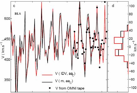
Variations in the Open Solar Magnetic Flux 13

2.3 Dependencies of the various indices on interplanetary parameters
In-situ spacecraft data on the near-Earth interplanetary medium became increasingly available
from 1963, at the start of the space age. Early studies comparing geomagnetic activity to the
near-Earth interplanetary parameters (e.g., Arnoldy, 1971) showed that geomagnetic activity was
enhanced when the interplanetary magnetic field (IMF) pointed southward in a reference frame
aligned by Earth’s magnetic axis: Geocentric Solar Magnetospheric, GSM, is widely used (Russell,
1971; Hapgood, 1992). This had been predicted in the seminal paper by Dungey (1961), who
proposed that for this IMF orientation, magnetic reconnection in the dayside magnetopause current
sheet would allow the solar wind to drive stronger F-region ionospheric flows (convection) and hence
the associated E-region ionospheric currents and geomagnetic activity seen at Earth’s surface would
also be stronger. The southward IMF orientation in GSM occurs for 50% of the time (Hapgood
et al., 1991). The DP2 or “directly driven” currents respond to IMF variations with a lag of
a few minutes (Nishida, 1968), whereas the larger DP1 or “storage-release system” currents are
enhanced during substorm expansion phases following a lag of typically one hour (e.g., Baker
et al., 1981). The high latitude auroral currents link to the magnetospheric ring current via the
Region-2 field-aligned currents, as shown in Figure 2. The ring current has long been understood
in terms of injection and decay of the trapped particles that carry it (Burton et al., 1975) and the
injection is more efficient when the interplanetary magnetic field points southward (see, e.g., Shi
et al., 2012). The response is complicated by the fact that the interplanetary electric field also
influences the decay of the ring current and there are other, internal magnetospheric factors which
influence both the injection and the decay (see reviews by Kozyra and Liemohn, 2003; Pulkkinen,
2007). Enhancements of the ring current cause negative depressions in the index but will also
influence other geomagnetic indices.
 Figure 3 explores the dependence, on annual averaging timescales, of the geomagnetic indices
described on Sections 2.1 and 2.2 on the solar wind speed, SW . The correlation between each
 
index and SW is presented where is the IMF field strength and is an exponent that is here
varied between –2 and 4. The correlations are for annual means between 1966 and 2012, inclusive.
Parameters marked with a prime denote that data have been omitted in computing both sets of
annual means if any of the simultaneous (allowing for the predicted satellite-to-Earth solar wind
propagation lag) hourly means of , SW or the geomagnetic index are missing due to a data
gap. In the case of the 3-hour range indices , and , the procedure adopted by Finch and
Lockwood (2007) is followed to ensure only simultaneous geomagnetic and IMF data are included
in the annual means. In the case of (1 ), each daily value contains information on from two
whole days: in order to be included in the annual means, we here require that there be 75% coverage
of the IMF observations over those two days. The value of 75% is chosen as a compromise between
not eliminating too much of the data and removing data for which the interplanetary means could
be misleading because the data coverage is low. The effects of not carrying out this piecewise
removal of data from both sets during datagaps were studied by Finch and Lockwood (2007):
effectively one is assuming that annual means are representative, even when large fractions of the
data are missing (as they are in some years for the interplanetary data). Even with the piecewise
removal of data during data gaps, we here only employ annual means that have data availability
exceeding 50% to avoid years of reduced data having undue weight. In the study presented in
Figure 3, all the correlations are somewhat improved by taking these steps and, importantly, the
 of peak correlation is sometimes also affected. Note that only annual mean data for and
 have been published and the way is generated only yields annual values: as a result, no
allowance for gaps in the interplanetary data can be made in these three cases (hence there is no
prime symbol attached to , , or in Figure 3).
 
 The coupling functions SW have been calculated in hourly data and then averaged, so that
⟨ SW ⟩1 yr is used rather than ⟨ ⟩1 yr (⟨ SW ⟩1 yr ) . The auroral electrojet index (red line)
 
 Living Reviews in Solar Physics
 http://www.livingreviews.org/lrsp-2013-4

14 Mike Lockwood

 1

 0.9
 correlation with [BVSW
 n
 ]′

 0.8

 Ap′
 0.7 −AL′
 AU′
 −Dst′
 −Dst1′
 0.6
 aa′
 IDV(1d)′
 IDV
 0.5 m
 Am′
 IHV
 −2 −1 0 1 2 3 4
 exponent of VSW, n

Figure 3: Linear correlation coefficients of annual means of various geomagnetic indices with SW , as
a function of , the exponent of the solar wind speed, SW ( is the IMF field strength). The primes
denote the fact that data have been omitted in calculating either set of annual means if any of SW , or
 
the geomagnetic index are missing because of data gaps exceeding 1 hour duration. Values of SW are
computed hourly and then averaged. Correlograms are shown for: (red line) ; (green line) ; (blue
solid line) − ; (blue dashed line) the negative part of , − 1 (where 1 is the same as but
intervals when > 0 are treated as data gaps); (cyan) ; (orange) ; (black dashed) ; (black
solid line) (1 ); (mauve) ; (yellow) and (red dashed) . For indices which are increasingly
negative for increasing activity ( , 1 and ) the index has been multiplied by −1. Image reproduced
from Lockwood et al. (2013a).

 2
shows peak correlation = 2, i.e., it has a SW dependence. The index (green line) gives a
peak at = 1.1 (i.e., it has close to a SW dependence and, hence, varies with the interplanetary
electric field). The index shows a peak at = 0.4 (blue line) but some of this dependence on
 SW arises from the compression of the equatorial field by enhanced solar wind dynamic pressure:
if we use only the negative part of ( 1 , which is the same as but treats all intervals
where > 0 as data gaps and so only contains intervals when is dominated by ring current
effects), we get the dashed blue line with a higher correlation coefficient peak at = 0.1. This
peak is flat and, hence, the peak is not significantly different from zero (i.e., the dependence is
 2
on alone). The cyan line is for the index and peaks at = 1.9 (very close to the SW
dependence of ), the mauve line is for and peaks at = 1.8 and the orange line is for 
and peaks at = 1.6. The black line is for the (1 ) index, which peaks at near −0.1. Hence
 (1 ), like and 1 , is not significantly different from having a dependence on only.
Thus, as concluded by Svalgaard and Cliver (2010), the negative part of (i.e., ring current
enhancement) is closest to explaining the behaviour of the interdiurnal variability indices on these
annual timescales. The range indices, and respond in a manner similar to the auroral indices
and, in particular, the influence of the westward auroral electrojet on (as monitored by )
can be inferred from the fact that both have a dependence that is not significantly different from
 2
 SW . The correlation for peaks at a slightly lower than for , , or , which may
be a greater influence of the directly-driven currents or may be the effect of the ring current (as
both and give peaks at lower ). The index correlation peaks at = 1.9 and so, as

Living Reviews in Solar Physics
http://www.livingreviews.org/lrsp-2013-4

Variations in the Open Solar Magnetic Flux 15

pointed out by Svalgaard et al. (2003) and Svalgaard and Cliver (2007a), behaves very much like
 2
 and all the range indices with a SW dependence, as expected because it is a monitor of the
nightside auroral electrojet.
 The index (yellow line) correlation peaks at = 0.3 and there are a number of possible
reasons why this value of exceeds zero. It could be that the response of is set by a mixture
of the ring current (with its = 0 dependence) and the DP2 auroral currents (with their = 1
dependence). An alternative explanation is that the normalisation against the index in the
derivation of has introduced a small dependence on SW . We also note that employed data
 2
from some auroral stations such as Sodankylä, which, as discussed in Section 6, introduces a SW
dependence into values.

3 The Long-Term Variability of Geomagnetic Activity
The first homogeneous, long-term record of geomagnetic activity was the index compiled by
Mayaud, who analysed 100 years’ data (1868 – 1968) from observatories in southern England and
near their antipodal locations in Australia (Mayaud, 1971, 1972, 1980). In each hemisphere, three
different stations were required to make a continuous record and, as for all such composites, inter-
calibration problems between the different stations arise. Means over calendar years and over
27-day Bartels solar rotation intervals are plotted in the top panel of Figure 4. When was first
used to reconstruct the solar magnetic fields, there were several vociferous objections that, despite
Mayaud’s careful calibration work, the drift seen in Figure 4 was merely an instrumental artefact.
There are, indeed, a great many problems that can cause long-term changes in the record from
a magnetometer station: in addition to instrument changes, drifts and re-adjustments, a change
in the local water table can have an influence, as can the construction of power or railway lines
nearby and, on very long timescales, the secular drift in the magnetic poles of the Earth causes
the geomagnetic coordinates of a station to drift. The argument that the values could not be
as low as derived around 1900 by Mayaud has been proved to be wrong by the recent long and low
solar minimum between solar cycles 23 and 24 (Russell et al., 2010; Lockwood, 2010). During this
minimum (around 2008), comparably low annual mean was observed, as is shown by Figure 4.
Analyses suggesting calibration problems were often based on comparisons with hourly mean data
(Svalgaard et al., 2004; Svalgaard and Cliver, 2005; Mursula and Martini, 2007). However, it has
become clear that hourly mean data are not observing the same mix of currents and phenomena
as the range indices (see Section 6) and, hence, many of the differences are real rather than
instrumental. This is underlined by the bottom panel of Figure 4, which shows the corresponding
means for another homogeneously-constructed long-term index, (1 ). Although many features
can be seen in both indices, there are many differences, particularly in the 27-day means. The
long-term change is seen in both indices despite 3 major differences between them: (1) they are
constructed using data from entirely different observatories, (2) one uses hourly means and the
other range data, and (3) the compilation algorithms (including the removal of quite day variations
and secular change in station latitudes) are entirely different. The correlation coefficients between
 and (1 ) for 27-data and annual means (for 1868 – 2013) are 0.68 and 0.76, respectively.
These correlations should be compared with those over the same interval between the independent
 indices for the northern and southern hemispheres, and , which are 0.94 for the 27-day
means and 0.98 for the annual means.
 A number of tests on have been carried out (e.g., Lockwood, 2001; Clilverd et al., 2002; Cliver
and Ling, 2002; Lockwood, 2003; Clilverd et al., 2005; Lockwood et al., 2006b; Lu et al., 2012)
which show it to be a reasonable indicator of long-term change. Furthermore, studies of potential
factors identified a solar origin of the long-term drift (Clilverd et al., 1998; Stamper et al., 1999;
Clilverd et al., 2002). However, there is also evidence of some error in the index, as stored in

 Living Reviews in Solar Physics
 http://www.livingreviews.org/lrsp-2013-4

16 Mike Lockwood

 60
 Greenwich
 50 & Melbourne
 Greenwich
 40 & Toolangi
 aa (nT)

 Abinger
 30 & Toolangi
 Hartland
 20 & Toolangi

 10 Hartland
 & Canberra

 Helsinki
 20 Niemegk
 IDV(1d) (nT)

 Eskdalemuir
 15

 10

 5

 1840 1860 1880 1900 1920 1940 1960 1980 2000
 year

Figure 4: Averages over Bartels 27-day solar rotation intervals (coloured) and calendar years (in black)
of (top) the geomagnetic index and (bottom) the (1 ) index. The colours give the station(s)
contributing the data to the indices at any one time. This version of the index is as stored in the
World Data Centres. The data labelled Niemegk are a composite from the three nearby stations, Niemegk,
Potsdam, and Seddin.

most data centres at the present time. The first authors to suggest errors in were Svalgaard
et al. (2004) who compared against the index: indeed they argued that all centennial
change in was erroneous. Comparing with is a valid test of because, as shown in
 
Figure 3, they both correlate best with SW for near 2. The initial comparisons by Svalgaard
et al. (2004) found an almost negligible change in since 1900 which would imply early 
values were too low: quantitatively they found the mean error in was 8.1 nT over solar cycle
14 (1901 – 1912, inclusive), which considering that the mean over this cycle was lower than the
mean for cycles 20, 21, and 22 by the same amount, means that they argued that all the long-term
change in was erroneous. However, this early version of was based on just one composite
data series from two very nearby stations, Cheltenham and Fredricksburg (intercalibrated using
the available 0.75 yr of overlapping data in 1956). Using more stations, Mursula et al. (2004)
found there was upward drift in values over the 20th century, but it depended on the station
studied; nevertheless they inferred that the drift in was too large. As a result, Svalgaard et al.
(2003) revised their estimates, using several stations, such that the cycle-14 mean of was too
low by 5.2 nT (this would mean that 64% of the drift in was erroneous). However, Mursula and
Martini (2006) showed that about half of this difference was actually in the estimates not
 and was caused by the use of spot values rather than hourly means in constructing the early
 data. This was corrected by Svalgaard and Cliver (2007a) who revised their estimate of the
difference further downward to 3 nT. These authors also showed that most of the difference arose
in a 6-year interval around 1957, which is the time of the move of the northern hemisphere 
station from Abinger to Hartland. Independently, Lockwood et al. (2006b) carried out tests of 
using the range index which has been constructed since 1936 from 11 – 13 northern hemisphere
stations, and range indices from a number of other stations (thereby ensuring that they were
comparing like-with-like). They also found a step-like change around 1957 and estimated it to
be about 2 nT in magnitude. Because 1957 was only 11 years before the end of the data series

Living Reviews in Solar Physics
http://www.livingreviews.org/lrsp-2013-4

Variations in the Open Solar Magnetic Flux 17

 35

 30

 25
 aa (nT)

 20

 15
 aa
 10 aac Ap
 aamax>aa>aamin
 5
 1880 1900 1920 1940 1960 1980 2000
 Year

Figure 5: Comparison of annual means of the standard index (in red) and the modified version 
derived by Lockwood et al. (2006b) (in blue). The estimated maximum uncertainty, relative to modern
values, is shown by the grey band. The green dots are annual means of the index.

available to Mayaud and because in that time solar cycle 20 was rather unusual, this discontinuity
in was not as apparent in the original data as it is now. Other studies also indicate that
 needs adjusting by about 2 nT at this date (Jarvis, 2004; Martini et al., 2012). The 2 nT
discontinuity estimate corresponds to an error in the drift in between cycle 14 and the space
age of about 25%. Lockwood et al. (2006b) implemented revised calibrations between stations (the
largest change needed being for 1957) and, hence, derived a revised index series . Figure 5
shows that the difference between annual means of and is generally less than 2 nT, which
is considerably smaller than the range of the long-term drift in annual means over the last 150
years (approximately 12 nT at sunspot minimum and 16 nT at sunspot maximum).
 Many historic datasets exist in the form of hourly mean data (or in the case of some of the
earliest data, spot values within the hour) and these have recently also been used to generate
indices. Until recently many were in the form of paper records in observatory yearbooks. However,
in recent years many have been digitised making a valuable new extra resource for reconstruction
work.
 Figure 6 shoes the variation of the “median index”, (Lockwood et al., 2006b). The construc-
tion of this index recognises that the response to global geomagnetic activity at a given observatory
depends upon its magnetic local time (MLT) and, hence, on the Universal Time (UT). However,
the station gives information at all UT and so rather than discard data from all but one MLT,
the index treats each station-UT as a separate data series. To avoid outliers having a dispro-
portionate effect, is defined as the median of all the normalised annual values for the different
station-UT combinations. The black line in the upper panel of Figure 6 is , which also shows a
similar long-term variation to the annual means of and (1 ) shown in Figure 4.
 Figure 7 shows the index compiled by Svalgaard and Cliver (2010). These authors take
the series back to 1835, just 3 years after the establishment of the first magnetic observatory in
Göttingen. This is done using a linear correlation between proper and the index. However,
it must be remembered that is not an inter-diurnal variability index before 1872 and Bartels did
not regard all the data before this date as reliable. Figure 7 also shows the variation in , the
number of stations used to compile .

 Living Reviews in Solar Physics
 http://www.livingreviews.org/lrsp-2013-4

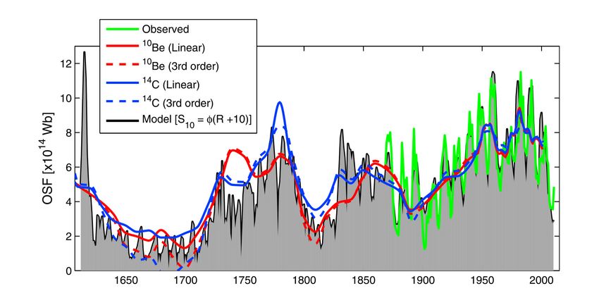
18 Mike Lockwood

 55
 Individual station−UT
 50
 Median, m

 45

 40

 35
[aa]∆H (nT)

 30

 25

 20

 15

 10

 5

 0
 300
 number of station−UTs
 200 number with r > 0.5

 100

 0
 1900 1920 1940 1960 1980 2000
 Year

Figure 6: The median index, . For each station at a given UT, the standard deviation of the hourly
means of the horizontal component of the geomagnetic field is computed over a full year, 1 yr . These are
then correlated with, and linearly regressed against, the annual means of aa shown in Figure 4 to yield
 ′ = × 1 yr + . These normalisations are needed because both the sensitivity and offset for a station
have been shown to depend on its location and on the UT hour (which, for example, alters the location of
the station relative to the midnight-sector auroral oval) (Finch, 2008). Each station-UT is treated as an
independent data series. The grey lines show the variations of the ′ values for all station-UTs for which
the correlation coefficient exceeds 0.5 and is significant at the 2 level. The number of station-UTs meeting
this criterion is shown as a function of time by the black histogram in the lower panel. The black line in
the upper panel is the median of all the available data for each year and is called the “median index”, .
Image reproduced from Lockwood et al. (2006b).

Living Reviews in Solar Physics
http://www.livingreviews.org/lrsp-2013-4

Variations in the Open Solar Magnetic Flux 19

Figure 7: Annual means of the index compiled by Svalgaard and Cliver (2010). The grey curves
are the variations for individual stations. The red curve is the index, defined as the arithmetic mean of the
median and average values of the individual station values. A few station values were very large outliers of
the distribution at any one time and those that were more than five standard deviations from the average
were omitted in calculating the value for that year. The number of contributing stations, , is shown
by the thin blue curve. The dashed blue line is the corresponding number of stations used by Svalgaard
and Cliver (2005). Bartels’ index is considered a single station and gives the dotted line extension to
before 1871 using a linear regression of 1871 – 1930 data with the index proper. Image reproduced
by permission from Svalgaard and Cliver (2010), copyright by AGU.

 Living Reviews in Solar Physics
 http://www.livingreviews.org/lrsp-2013-4

20 Mike Lockwood

 Note that for both and , the number of stations used decreases as one goes back in time,
which contrasts with Mayaud’s philosophy for which was to derive a homogeneously-constructed
data series. Given the potential for site-dependent errors and drifts, these indices therefore become
increasingly unreliable as one goes further back in time. Svalgaard and Cliver (2010) state that
“only a few (good) stations are needed for a robust determination of ”. This is indeed a
valid statement: for example, (1 ) (shown in the bottom panel Figure 4) is based on just
one station at any one time, yet for 1880 – 2013 it gives a correlation coefficient of 0.96 with 
(Lockwood et al., 2013a). However, before 1880 the correlation is considerably lower. Svalgaard
and Cliver (2010) note that they had to discard some data because they were more than 5 from
the mean. This poses a dilemma if there are too few stations to define the distribution: in such
cases these outliers could not be identified and one would have used them, not knowing they were
in error. In other words, without sufficient other stations to compare with, one is not able to say
which the “good” stations are. It therefore is inevitable that the inhomogeneous data series such as
 and are less reliable further back in history. Potential causes of additional uncertainty in
early data are: (1) there were fewer stations; (2) measurement techniques and equipment improved
with time; (3) the realisation of that urban environments were generating magnetic noise problems
forced moves to quieter observing sites; and (4) earlier data tend to be spot values rather than
hourly means. On the last point, Svalgaard and Cliver (2010) could find no discontinuities in the
 data series from individual stations (unlike values) when they changed from supplying
spot values to hourly means. Nevertheless, it is self-evidently true that hourly means are preferable
to spot values, particularly if a site is suffering from any intermittent noise problems and/or if the
instrument stability is poorer.
 Figures 4, 6, and 7 all show similar long-term variations, despite the fact that the indices pre-
sented differ in almost every facet of their compilation. There are, however, important differences
that are discussed in Section 6. These data from geomagnetic observatories give an invaluable re-
source for studying solar-terrestrial physics and solar variability in the 181 years since Gauss’ first
observatory was established in Göttingen. In particular, we can study the variations in the solar
corona and interplanetary medium that accompany the long-term sunspot variations identified by
Gleissberg (1944). Feynman and Crooker (1978) studied the implications of the drift in the in-
dex and concluded that either the solar wind speed or the IMF had changed over the past century.
The first paper to separate these two influences (using the recurrence index of Sargent, 1986, to
quantify solar wind speed), thereby showing that the main change was in the magnetic field, was
by Lockwood et al. (1999a). These authors used to reconstruct the unsigned open solar flux,
which is the total magnetic flux leaving the top of the solar corona and entering the heliosphere.
Other solar terrestrial phenomena, such as lower latitude auroras, were found to reveal the same
long term changes as and the derived open solar flux (for example, Pulkkinen et al., 2001).

Living Reviews in Solar Physics
http://www.livingreviews.org/lrsp-2013-4