POTENTIAL FOR SOLAR ENERGY ON ROOFTOPS IN THE MUNICIPALITY OF UPPSALA - JASMINE HAMMAM SARA JOHANSSON HANNA PERSSON - DIVA PORTAL
←
→
Page content transcription
If your browser does not render page correctly, please read the page content below
Examensarbete 15 hp
                                  Juni 2013

Potential for Solar Energy on
Rooftops in the Municipality of
Uppsala

Jasmine Hammam
Sara Johansson
Hanna Persson
Abstract
Potential for Solar Energy on Rooftops in the
Municipality of Uppsala
Jasmine Hammam, Sara Johansson, Hanna Persson
Teknisk- naturvetenskaplig fakultet
UTH-enheten Uppsala City Council has set up milestones for each decade from year 2020 to 2050
to steadily reduce the greenhouse gas emissions per capita in the municipality of
Besöksadress: Uppsala. The Climate Protocol is working on a roadmap with guidelines on how to
Ångströmlaboratoriet
Lägerhyddsvägen 1 achieve the current climate goals. The roadmap is expected to be finished in year
Hus 4, Plan 0 2014, and it is currently being investigated to what extent solar energy could
contribute to achieving the climate goals. The purpose of this study is to estimate the
Postadress: solar energy potential in the municipality of Uppsala for the years 2020 and 2050
Box 536
751 21 Uppsala based on an assessment of what a prospective utilization of solar energy systems on
rooftops could potentially generate. The addressed solar techniques are photovoltaics
Telefon: based systems and solar thermal collectors.
018 – 471 30 03 The results indicate that an optimal rooftop area of 5.9 km² is estimated in Uppsala
Telefax: municipality by 2020, and 8.8 km² by 2050. The total solar energy potential in the
018 – 471 30 00 municipality is estimated to 1.5 TWh in 2020 and 1.9 TWh in 2050. Thus,
approximately half of all the buildings energy consumption in the municipality could
Hemsida: potentially be covered by solar energy.
http://www.teknat.uu.se/student
A sensitivity analysis is carried out to test the results by altering input parameters and
components. The sensitivity analysis indicates that the solar energy potential would
increase by optimizing roof deployment areas when constructing new buildings and
improving the solar efficiency for photovoltaics. The results indicate that solar energy
could cover 49 percent of the municipality’s expected energy demand in 2020 and 64
percent in 2050.
Handledare: Björn Sigurdson
Ämnesgranskare: David Lingfors
Examinator: Joakim Widén
ISSN: 1650-8319, TVE 13 006 majTable of contents
1.! Introduction .......................................................................................................................... 9!
1.1! Purpose ........................................................................................................................ 10!
1.2! Terminological clarification ........................................................................................... 10!
1.3! Limitations..................................................................................................................... 10!
1.4! Report outline ............................................................................................................... 11!
2.! Background ........................................................................................................................ 12!
2.1! Climate goals of Uppsala Municipality .......................................................................... 12!
2.2! Active solar energy systems ......................................................................................... 13!
3.! System view ....................................................................................................................... 14!
3.1! Grid parity ..................................................................................................................... 15!
4.! Methodology ...................................................................................................................... 16!
4.1! Building types and estimated roof surfaces .................................................................. 17!
4.2! Roof angles................................................................................................................... 18!
4.3! Azimuth angle ............................................................................................................... 19!
4.4! Shading and obstacles on roof areas ........................................................................... 20!
4.5! Solar calculations.......................................................................................................... 21!
4.5.1! Calculating the solar efficiency ............................................................................. 21!
4.5.2! Solar power output from a tilted surface ............................................................... 22!
4.6! Future scenarios ........................................................................................................... 23!
5.! Data ..................................................................................................................................... 24!
5.1! Future constructions in the municipality........................................................................ 24!
5.2! Cultural and historical values ........................................................................................ 25!
5.3! Estimated number of buildings and ground area .......................................................... 25!
5.3.1! Buildings suitable for solar energy systems ......................................................... 26!
5.4! The energy consumption in the municipality................................................................. 28!
6.! Sensitivity analysis for 2020 and 2050 ............................................................................ 29!
6.1! Roof angle .................................................................................................................... 29!
6.2! Azimuth angle ............................................................................................................... 29!
6.3! Shading and obstacles ................................................................................................. 29!
6.4! Improved efficiency ....................................................................................................... 30!
6.5! Estimated roof area of new buildings 2020 to 2050...................................................... 31!
7.! Results ................................................................................................................................ 32!
7.1! Roof area calculations .................................................................................................. 32!
7.2! Solar energy potential ................................................................................................... 34!
7.3! Sensitivity analysis........................................................................................................ 35!
7.4! Comparison of the two scenarios ................................................................................. 36!
8.! Discussion .......................................................................................................................... 37!
3
!8.1! Results .......................................................................................................................... 37!
8.2! Sensitivity analysis........................................................................................................ 37!
8.3! Critical analysis ............................................................................................................. 37!
8.4! A future outlook............................................................................................................. 38!
8.5! Further work.................................................................................................................. 40!
9.! Conclusions ....................................................................................................................... 41!
10.! References ....................................................................................................................... 42!
10.1! Literature..................................................................................................................... 42!
10.2! Publications ................................................................................................................ 42!
10.3! Web sites .................................................................................................................... 44!
10.4! Other references ......................................................................................................... 46!
Appendix: Solar Energy Potentials ......................................................................................... 47!
!
!
4
!Occurring Terms and Abbreviations
Apartment buildings Buildings with several households (apartments) under the
same roof, estimated to 14.55 apartments per building.
Azimuth The facilities orientation relative to the south. Directly to the
south gives 0 degrees, west 90 degrees and east -90 degrees.
Diffuse radiation Particles and clouds scatter the solar radiation to be
distributed over the entire hemisphere.
Direct radiation See definition for Solar Radiation.
GI Global Irradiance, solar radiation on module plane.
η Solar cells efficiency rate, measured in percent.
NOCT Nominal Operating Cell Temperature, used to determine cell
efficiency
Module Collection of photovoltaic arrays, also called panels
PV Photovoltaic, direct conversion of solar radiation to
electricity.
Small houses Refers to individual, detached and semi-detached homes
such as villas, cottages and town houses.
Solar radiation The solar energy reaching a given area in a given time,
commonly measured in kWh/m², diffused or direct. When
the sun is in the zenith, 90 degrees angle, the direct solar
radiation is at maximum.
Solar thermal Conversion of sun radiation to heat.
STC Standard Test Conditions, used to determine cell efficiency.
Sustainable development "Development that meets the needs of the present without
compromising the ability of future generations to meet their
own needs." - from the World Commission on Environment
and Developments.
5
!System Components that are united to a whole, for example a PV
system consists of all parts needed for installing and
producing electricity.
Tc Solar cell temperature
! !
6
!List of Figures
Figure 1 Forecast on greenhouse gas reductions per capita p. 12
Figure 2 Map of heating network district p. 14
Figure 3 Flowchart over the model used in this study p. 17
Figure 4 Illustration of an ideal building p. 18
Figure 5 Illustration of the tilted solar module p. 19
Figure 6 Example of azimuth angle p. 20
Figure 7 Illustration of angles for solar calculations p. 22
Figure 8 Estimated number of buildings 2012 to 2050 p. 25
Figure 9 Estimated ground areas 2020 to 2050 p. 26
Figure 10 Estimated number of buildings available for solar thermal p. 27
Figure 11 Estimated number of buildings available for PV p. 27
Figure 12 Energy consumption p. 28
Figure 13 Optimized azimuth angle p. 29
Figure 14 Newly constructed roof area, built 2020 to 2050 p. 31
Figure 15 Calculated roof areas for different building types p. 32
Figure 16 Estimated roof area available for solar thermal p. 33
Figure 17 Estimated roof area available for PV p. 34
Figure 18 The solar energy potential p. 34
Figure 19 The solar energy potential in the sensitivity analysis p. 35
Figure 20 Comparison of the energy usage and solar energy potential p. 36
Figure 21 Illustration of the influence of factors on the solar energy potential p. 36
7
!List of Tables
Table 1 Average reductions in tonne greenhouse gases p. 13
Table 2 Roof and solar cell angle on different building types p. 19
Table 3 Reduction percentage due to obstacles and shading p. 20
Table 4 Optimized roof and solar cell angle, buildings built 2020 to 2050 p. 29
Table 5 Optimized reductions for different buildings built 2020 to 2050 p. 30
Table 6 PV module area for industry buildings 2012-2050 (km2) p. 34
8
!1. Introduction
Emissions of greenhouse gases have increased on Earth as a result of human activities
during the past centuries. The Earth’s average temperature is projected to increase over
the next 100 years if the emissions continue unchanged (Solomon et al. 2007). The
International Energy Agency, IEA, states that ”improved energy efficiency is often the
most economic and readily available means of improving energy security efficiency and
reducing greenhouse gas emissions “(IEA, 2008).
To reduce energy consumption and greenhouse gas emissions has the municipality of
Uppsala set up climate goals until 2050 based on roadmaps from the European Union
and the Swedish government. One of the climate goals formulated by the Uppsala City
Council is to reduce the greenhouse gases per capita from 6.2 tonne per capita in 2012
to 0.5 tonne per capita in 2050. (Sandström and Sigurdsson, 2011). In order to achieve
this goal by 2050, the municipality expects to gradually reduce its dependency on fossil
fuels and move towards a fossil-fuel free society (Sigurdsson, 2013b). This will require
investments in renewable energy sources and finding alternatives that could phase out
and eventually replace fossil fuels completely. Uppsala has investigated the possibility
of building wind farms in the municipality but has encountered problems, due to the risk
of forming air barriers interfering with activities of the military air force deployed near
Uppsala (Provincial government, 2011). Therefore other options are now being
examined, with a growing interest for solar energy. Utilization of solar power has in
recent years become a more attractive option, as it is a renewable and unlimited energy
resource. With a steadily improving technology and lowered costs, the interest in solar
energy is accelerating worldwide (Solenergi, 2013).
The Uppsala Climate Protocol, an initiative of the municipality of Uppsala, was
founded in 2010 and is a cross-industry cooperation on energy efficiency and climate
change. The members consist of local businesses, government- and non-government
organizations. The Climate Protocol is divided into several focus groups with different
areas of interest, all together contributing to the municipality’s efforts in establishing a
roadmap specifying the steps for successfully achieving the climate goals for 2020 and
2050. One focus group is promoting initiatives exploring the area of solar energy in the
municipality. (Sandström and Sigurdsson, 2011) The aim of this study is to provide
means for the focus group to evaluate the prospects for solar energy in the municipality
of Uppsala.
9
!1.1 Purpose
The purpose of this study is to estimate the solar energy potential in Uppsala
municipality from 2020 to 2050 based on an assumption of prospective utilization of
rooftops for solar power generation.
The following will be addressed:
! Estimation of the amount of rooftop area in the municipality, which is suitable
for the deployment of solar energy production (photovoltaics and solar thermal).
! Estimation of the amount of energy that could be produced through the projected
rooftop utilization.
! Estimate to what extent solar energy can contribute to cover the future energy
needs in the municipality of Uppsala.
1.2 Terminological clarification
The term solar energy potential can be interpreted in different ways, for example,
surface potential, technical potential or market potential. This study concerns the
technical potential based on current technically feasible solutions (Kjellson, 1999). A
sensitivity analysis is provided wherein a higher cell efficiency is explored. Additional
input parameters are also modified to demonstrate levels/limits of an alternative
scenario. A comparison is made between the results from the two scenarios to gauge the
importance of different parameters on the solar energy potential.
1.3 Limitations
There are a number of limitations in the study. Firstly, the total solar energy potential
for the municipality is calculated through the simulation of solar modules on rooftops.
Facades and other possible areas, demolition of buildings or already deployed solar
systems in the municipality is not taken into account. The performance of the solar
modules is assumed to be stable throughout their lifespan. It is assumed that the solar
devices are connected in parallel, to avoid the risk of total system failure, when partly
shadowed.
No calculations are made on the economic aspects of a photovoltaic and solar thermal
expansion in the municipality, nor is the possibility of selling or feeding surplus power
into the electrical grid analyzed. Some economic aspects are however briefly discussed
in qualitative terms in the system view section and in the discussion section to provide
an understanding of the economic dynamics involved when studying prospective wide
implementation of solar energy systems.
10
!The study does not include a Life Cycle Analysis. Emissions and energy losses caused
in the production process, installation, usage or transportation of the solar devices are
not addressed. Any negative effects on the solar plants caused by wear, such as
exposure of snow or dirt is not considered. Lastly, possible climate change that could
influence the energy demand in Uppsala is not considered. The average temperature and
solar radiation in year 2020 and 2050 is assumed to be the same as the average values of
today.
1.4 Report outline
The report begins with a background section which is divided into three parts: an
introduction climate goals of the municipality of Uppsala and the work of the Uppsala
Climate Protocol, a presentation of solar energy systems and a brief explanation of the
concept grid parity. In Section 4, the methodology used to calculate the solar energy
potential is presented and followed by data in section 5, including the assumptions made
for the different scenarios. Section 6 consists of a sensitivity analysis where input
parameters are changed. The results of the simulations are presented in section 7. Lastly,
in section 8 the report ends with a discussion of the results, along with a number of
conclusions in section 9.
11
!2. Background
2.1 Climate goals of Uppsala Municipality
In a strategy plan from 2011, the municipality of Uppsala formulated a set of long-term
climate goals to promote a resource efficient and climate neutral energy system for the
municipality. The climate goals described in the strategy plan are based on goals
specified by the European Commission and includes a time plan of how the
municipality gradually should reduce the amount of carbon dioxide per capita until
2050. The time plan is shown in Figure 1. The emissions per capita are estimated to
drop from 6.2 tonne per capita in 2012 to 0.5 in 2050. In the graph it is displayed how
the total emissions of greenhouse gases from the energy sector, other emission sources,
and long distance travelling has to decrease to achieve the existing climate goals set to
2050. (Sandström and Sigurdsson, 2011)
Greenhouse)Gas)Emissions))
Greenhouse)gas)emissions)in)tonne)per)capita)
10!
Milestone:!Long7distance!travel!
9!
8!
7! Milestone:!Other!emissions!
6!
5! Milestone:!Energy!and!
4! transport!
3!
2! Long7distance!travel!
1!
0! Other!emission!sources!
Energy!and!transport!
Figure 1. The chart illustrates a forecast on how greenhouse gases per capita should
reduce within the municipality until 2050 (Municipality of Uppsala, 2012a).
As shown in Figure 1, considerable reductions of greenhouse gas emissions in
electricity, heating and transport will be required in order to achieve the municipality’s
climate goals. Such reductions would yield the following average reductions in tonne
greenhouse gases per capita compared to the levels in 1990, which is shown in Table 1.
(Sandström and Sigurdsson, 2011)
12
!Table 1. Average reductions in tonne greenhouse gases
(Sandström and Sigurdsson, 2011).
Year 2020 2030 2040 2050
Reduction 45% 65% 85% 95%
The above goal requires a large-scale transition from fossil fuels to alternative
renewable energy sources. Therefore, solar energy is being investigated by the
municipality’s solar focus group as an interesting alternative. (Municipality of Uppsala,
2012a)
2.2 Active solar energy systems
There are two main techniques used for solar energy. The first method is solar thermal
generation, based on using collectors to provide heat by absorption of solar radiation.
The heat can either be used for hot water stored in a hot water tank, or space heating
(Energy Saving Trust, 2013). The second method is called photovoltaics (PV), using
solar cells to convert photonic radiation directly into electricity. Solar cells are collected
in arrays and put together to create a solar module or PV system (Solcellforum, 2013).
All PV systems produce direct current, DC, and must be converted to alternating
current, AC (Nersesian, 2010, p. 325).
Solar energy systems can be used in many different areas, from meeting a buildings
electricity demand to lighting for signs, gardens and streets etc (Nersesian, 2010, p 329).
Solar cells and collectors can be integrated or mounted on both building rooftops and
facades and can therefore be used in rural areas and major cities without disturbing the
surrounding environment (Nersesian, 2010, pp. 323-324).
An important feature of renewable power sources such as solar power, wind power and
wave power, is variability. This feature is often described as the major obstacle to a
large-scale integration of renewable energy systems. (Widén, 2010) The main
variability for solar energy is consistent seasonal and diurnal fluctuations due to the
earth’s movement around its own axis and around the sun. The second source of
variability for renewable energy is weather conditions. (Widén, 2010 p. 35)
A common misconception is that high-latitude countries have a low solar radiation in
total. In fact, the solar radiation in Sweden, being a high-latitude country, is only
marginally lower than, for instance, in Central Europe. The main challenge is the more
pronounced annual variations of solar time during summer and winter and the lower
solar altitude during winter months. (Widén, 2010, pp. 26-27)
13
!3. System view
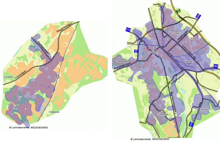
Most buildings in the proper city of Uppsala, and in a region of the municipality called
Storvreta, are connected to the district-heating network. The district heating is today
considered to be 80 percent renewable (Vattenfall, 2013a). Thus, solar modules on
rooftops could contribute as an additional renewable energy source for domestic
electricity. At the countryside however, investments in the solar thermal technique
could be more favorable as solar thermal modules can cover half of a household’s hot
water consumption (Byggmentor, 2013). Therefore, the municipality is divided into two
different parts in this study: the countryside and the urban area including Storvreta.
The study will investigate how much energy that could be generated by solar thermal at
the countryside and estimate the amount of additional electricity that solar modules
could generate in the city of Uppsala and in Storvreta. The number of buildings
connected to the heating network in Uppsala and Storvreta is in this study estimated to
about 10,300 small houses and 4,200 apartment buildings (Swedish Statistics,
2011)(Vattenfall, 2013b,c). Moreover, solar modules are as well assumed suitable on
rooftops of industries, facilities and unspecified buildings.
Figure 2. The maps show the district -heating network, colored in blue, where PV
installations are assumed. The map to the left illustrates Storvreta and to the right
Uppsala. (Vattenfall, 2013b,c)
14
!3.1 Grid parity
The combined effect of falling PV system costs and rising electricity bills in Europe has
made solar power more recognized as an attractive proposition (Lucia, 2013). Grid
parity is projected to be reached in many of the European countries by 2020, with costs
declining to about half of those of 2010 according to European Photovoltaic Industry
Association (EPIA, 2013, p. 4). The EPIA defines grid parity as:
“The moment at which, in a particular market segment in a specific country, the present
value of the long-term net earnings (considering revenues, savings, cost and
depreciation) of the electricity supply from a PV installation is equal to the long-term
cost of receiving traditionally produced and supplied power over the grid.”
(EPIA, 2013, p. 5)
Germany is one of the leading countries on the PV market and reached grid parity
already in 2011, making PV electricity generated from domestic roofs cheaper than
buying electricity from the grid in Germany. This was achieved through a combination
of subsidies supported by the government and the sharp fall in PV rooftop system prices
in recent years (Germany Trade and Invest, 2012, p.2). From year 2006 to 2011, there
was a 50 percent reduction in prices in PV technology (Solstats, 2011).
Today there is a general view that the falling trend in PV system costs will continue to
decrease in the future, as the price performance ratio is expected to go down further due
to technical improvement and factors related to economy of scale. It is also believed that
the prices of commercial systems could plummet by more than 40 percent by 2015, and
an additional 30 percent by 2020 (Aanesen, et al, 2012, p. 4). Even though subsidies are
expected to eventually disappear, the manufacturing capacity is expected to double over
the next 3 to 5 years and underlying costs to drop by as much as 10 percent annually
until 2020 (Aanesen et al, 2012, p. 2).
The Swedish solar market is growing, slowly, but growing. Statistics on the Swedish
PV market show that the system costs in Sweden continues to fall and the price
difference between venders is decreasing as well. (Lindahl, 2013) In Sweden, grid
parity is estimated to be reached for both residential and industrial markets by 2020
(Breyer and Gerlach, 2011).
!
15
!4. Methodology
The investigation is based on literature studies and results accumulated from using a
numerically based computational model implemented in MATLAB. Multiple-step
simulations calculate the annual solar energy potential in the municipality. To calculate
the total roof area in the municipality, ground area data collected from Statistics Sweden
(Statistiska Centralbyrån) is used together with assumptions of the roof inclines of five
different standard types of buildings. The ground area data is based on building
statistics for year 2011, but is assumed to be the same in 2012. To obtain the optimal
amount of roof area for mounting solar modules, a percentage reduction for shading and
obstacles on rooftops is made for each type of building. An additional percentage
reduction of number of buildings is made for cultural and historical buildings as they
are considered as unsuited for solar plants.
Exclusive usage of crystalline silicon solar cells and flat plate collectors are assumed in
this study, as these types are dominant on the market. This influences the assumptions
of solar efficiencies used in the calculations. Together with radiation calculations and
calculations mentioned in the paragraph above, a picture of the solar potential for 2020
and 2050 in the municipality is assembled. Meteonorm data for solar radiation and
ambient temperature data is collected from a normalized year, 1995 (Meteonorm, 2013).
The data is specified by the hour and extends over a year.
The year 2012 is used as a base year in this study. The results will be compared to the
total energy usage in Uppsala 2012, without using solar energy; in order to see how
much of the energy needs that could be covered by solar power. The following sections
describe the various working steps in more detail. Figure 3 illustrates a flowchart of the
model including all parameters that influences the output potential. The red blocks are
modified in the sensitivity analysis.
16
!Figure 3. A flowchart of the model used in this study. The red blocks are altered in the
sensitivity analysis.
4.1 Building types and estimated roof surfaces
In this study the following sectioning of different building types has been used:
! Small Houses
! Apartment buildings (possibly publicly owned respectively privately owned)
! Public facilities (municipality, county, church, military and so on)
! Private facilities
! Industry
! Unspecified
This sectioning is also used by Statistics Sweden and the Swedish Energy Authority
(Energimyndigheten). However, the category Unspecified buildings has been added for
this study, due to the high ratio of the total rooftop area which was received from
Uppsala Municipality (Statistics Sweden, 2011). Private and public facilities are in
some parts of this study added together in one category: facilities.
17
!In the calculations, it is assumed that all building categories have an ideal quadratic
shape. A model of the rooftops is shown in Figure 4.
Figure 4. The image displays the ideal building assumed when calculating of the roof
surfaces.
Equations for calculating roof area on one building:
!! = ! (1)
!
! = !! (!"#!!) (2)
!"#$!!ℎ!!!"!#$!!""#!!"#!! = !! ∗ ! (3)
4.2 Roof angles
The roof angle assumptions are based on results from a previous study of integrating PV
in Sweden written by Elisabeth Kjellsson (Kjellson, 1999). Based on Kjellsson’s roof
data, a 30-degree roof angle is assumed for all building types except for the industry
category, which is assumed to have a solar module tilt angle of 25 degrees.
18
!Table 2. The roof and solar module angles for different building types.
Building type Roof angle (α) Tilt angle (β)
Small houses, Apartment 30° 30°
buildings, Facilities,
Unspecified
Industry 0° 25°
!
For tilted rooftops it has been assumed that solar modules are installed directly on the
roof, while on flat roofs solar modules are installed with a tilting angle of 25 degrees.
The distance between the modules is assumed to be 2.4 meters and the width of the
modules to 1 meter to optimize the solar radiation (Näsvall, 2013). Figure 5 shows how
the modules are placed on flat roofs.
These equations are used for calculating the solar module area on flat roofs:
!
!! = ! ! (4)
!! = !! ∗ !!! ∗ ! !! (5)
Where Nm is the number of module rows and Am the module area.
Figure 5. The figure shows how the solar modules are placed on flat rooftops. In
equation (4) and (5), the variables S,W,d, β represents the house side, panel
width, distance between panels and the tilt angle respectively.
4.3 Azimuth angle
In the simulations only half of the roof surface has been considered for placement of
solar modules, as the south pointing roof surface is the most optimal placement. This
regards all the building types except for the industry category. As the solar radiation on
the roof surface depends on the buildings orientation, the building directions were
simulated in MATLAB between the intervals of -90 to 90 degrees, see Figure 6. Instead
of randomizing all the buildings different azimuth angles, the interval was divided into
six steps to save simulation time.
19
!Figure 6. The azimuth angle range for a building.
4.4 Shading and obstacles on roof areas
Shading and obstacles is another factor, which limits the amount of available roof area
for solar energy and can be caused by surrounding buildings, chimneys, ventilation
pipes or trees. The percentages for shading and obstacles are found in Table 3 and are
based on Kjellsson’s study for integrating PV in Sweden (Kjellson, 1999).
Table 3. Reduction percentage for roof areas due to obstacles and shading
(Kjellson, 1999).
Building type Reduction for obstacle Reduction for shading
Small houses, Private 10% 10%
facilities, Unspecified
Apartment buildings, 10% 15%
Public facilities
Industry 20% 10%
!
!
!
!
!
20
!4.5 Solar calculations
The following sections will describe how the solar efficiency and power output from a
tilted plane was calculated.
4.5.1 Calculating the solar efficiency
Today, an efficiency rate of 25-26 percent has been achieved in laboratories for the best
solar cells, (Solar AB, 2013) however, these solar cells are based on technologies,
which are at the moment prohibitively expensive for general deployment. A typical cell
efficiency rate for a commodity solar cell is about 17 percent (Swemodule, 2012). In
this study, the cell efficiency is set to 14 percent and is assumed to be stable with
respect to ageing. A conservatively low efficiency rate for crystalline solar cells has
been chosen to compensate for the assumed constant cell efficiency through out a
projected lifespan of 20 years.
The cell temperature is an important factor to consider when analyzing a solar cell
system. STC, Standard Test Conditions, is a general model designed to compare the
performance of the solar cell under standardized conditions. The starting point for a
given solar cell is always 25 °C. The efficiency of the solar cell drops by approximately
0.4 percent for each degree the cell temperature rises. (Zimmermann, 2013)
At standard conditions, the peak power or full module area efficiency is measured to:
! Solar insolation STC/GSTC = 1000 [W/m²]
! Air Mass, AM 1.5 spectrum
! Tc = 25°C
The path length of radiation passing through the atmosphere is described by the air
mass, AM (Widén, 2011). The air mass coefficient defines the direct optical path length
through the atmosphere. AM 1.5 corresponds to a solar zenith angle of θZ=48.2°.
(Zimmermann, 2013)
However, this does not exactly reflect reality. When operating in the field, solar cell
typically operate at higher temperatures and at slightly lower insolation conditions. It is
important to determine the expected operating temperature of the PV module, in order
to determine the power output of the solar cell. The Nominal Operating Cell
Temperature (NOCT) is defined under following conditions (PV education, 2013):
! Irradiance on cell surface = 800 W/m 2
! Air Temperature = 20°C
! Wind Velocity = 1 m/s
In this study the NOCT value is used for calculating the PV efficiency, as it is more
dynamic and accurate in comparison to STC. The efficiency rate of the PV system was
calculated with equation (3.16) on page 47 in “System Studies and Simulations of
Distributed Photovoltaics in Sweden” (Widén, 2010, p. 47).
21
!The efficiency for a solar collector is also temperature dependent and is calculated with
the equation:
(!!!! )
! = ! !! ! − !! ∗ !!
(6)
This equation is developed by Björn Karlsson, professor at Linköping University. The
optic efficiency is defined as η0. The heat loss factor is defined as U in the equation, T is
the temperature in the water tank set to 50 °C and Ta is the ambient temperature.
(Karlsson). The values for η0 and U are based on data for flat plate collectors (Viridan
Solar, 2013).
4.5.2 Solar power output from a tilted surface
To calculate the solar potential, the solar radiation on a tilted plane must be determined.
For this, equations (13) to (32) in “Solar Energy – Technology and Systems Solar
radiation Lecture Notes” were used. (Widén, 2011, pp. 16-22)
Figure 7. Illustration of the parameters used in the equation (13) and (32), which can
be found in Appendix I together with belonging values and units.
The final equation (32) uses the extraterrestrial radiation (I0), the beam radiation (IbT),
the diffuse radiation (IdT) and the ground reflected radiation (IgT) to calculate the total
solar radiation (IT). (Widén, 2011, pp. 16-22)
The power output of the PV system was calculated by using equation (3.17). Additional
array losses was predefined as qadd=0.01-1 C°. The efficiency of the inverter and other
equipment was predefined as ηe=0.9. (Widén, 2010, p. 47)
The power output of a solar collector was calculated with the formula:
! = !! ∗ !! ∗ !! (7)
22
!Where IT is the radiation on a tilted plane, Am is the module area and η is the efficiency
of the collector.
4.6 Future scenarios
The calculations are based on a number of assumptions of future scenarios in 2020 and
2050. These assumptions for the scenarios are listed below:
• Electricity from solar devices is assumed to have reached grid parity, meaning
that it is profitable to replace purchased electricity with solar power.
• Buildings connected to the district heating network is assumed to use solar cells,
while residents not connected to the district heating network use solar thermal.
• The number of buildings with cultural and historical value in the municipality
will not increase. This is described more in detail in section 5.2.2.
• By 2050, the electric grid has been re-modeled and adapted for extraction of
solar cells on a large scale.
23
!5. Data
5.1 Future constructions in the municipality
Since construction developers most often work on short-term building plans, the future
construction rate for small houses and apartment buildings is based on today’s
construction rate. According to prognosis provided by the provincial government, about
8,000 residential homes will be built in the urban areas and about 1,200 residential
homes in rural areas from year 2011 to 2016. (Provincial Government, 2012, p. 6) In
this study, it is assumed that apartment buildings are only built in the urban areas
whereas small houses are built in rural areas. With this assumption, the annual
construction rate is about 110 apartment buildings and 240 small houses. The
construction rate is assumed to be linear until 2050 based on the assumption that the
construction rate is well correlated with the population growth over time (Municipality
of Uppsala, 2012b). According to The Swedish National Board of Housing, Buildings
and Planning (Boverket), the average apartment building in Sweden has 14.55
apartment units per building. (Boverket, 2013) This value was used to extrapolate the
number of existing apartment buildings in the municipality of Uppsala.
Based on the municipality’s roadmap it is projected that 100,000 to 150,000 m² of office
space for trade purposes will be needed, and 200,000 to 250,000 m² floor space for
office purposes is needed until 2030 (Sandström and Sigurdsson, 2011). In this study it
is assumed that the entire surface for trade purposes and half of the space for office
purposes belongs to the private facility category. The average ground area for all
facilities is assumed to be 100 m². An additional 100,000 m² of floor space needs to be
built until 2030, along with another 112,500 m² of office space for public services
(Sandström and Sigurdsson, 2011). The ground area for public facilities in 2012 is about
623,000 m² and the normalized ground area for public facilities units is estimated to 100
m² as well.
Furthermore, the roadmap indicates that 400,000 m² of floor space for industries will be
built by 2030. The same amount of additional floor space is assumed by 2050,
compared to 2030. (Sandström and Sigurdsson, 2011) With the data for number of
industries and ground area 2012, an estimation of about 570 m² ground area per industry
is made. (Swedish Statistics, 2011)
About 6,300,000 m² of the total ground area for buildings in Uppsala 2012 consist of
unspecified buildings (Swedish Statistics, 2011). The average ground area for this
category is assumed to be 20 m². It is assumed that no additional unspecified buildings
are constructed until 2050.
24
!5.2 Cultural and historical values
From an architectural and historical point of view, there can be objections to the
deployment of solar energy systems. In the Planning and Building Act it is stated that
any changes of a building should take architectural, historical, cultural, environmental
and artistic values into account (Swedish law 1994:852). According to Kjellsson, 16
percent of the small houses, 9 percent of the apartments and 18 percent of today’s
facilities are of cultural or historical value (Kjellsson, 1999, pp. 28-29). The percentages
represent Sweden in general, but are directly applied for Uppsala as the percentages are
assumed to be representative extrapolations for Uppsala as well. Industries and
unspecified buildings are assumed to have no cultural or historical value in this study.
Furthermore, it is assumed that the number of buildings with historical or cultural value
will not increase.
5.3 Estimated number of buildings and ground area
The estimated number of buildings and ground areas in Uppsala municipality is shown
in Figure 8 and Figure 9. All ground areas for 2012 is based on data from Swedish
Statistics (Swedish Statistics, 2011).
Es7mated)Number)of)buildings)in)the)
Municipality)of)Uppsala)
380!
Number)of)buildings)in)thousands)
3!
370! 8!
360! 2!
1! 16! Industry!
350! 5!
4!
7! 9!
340! Apartment!buildings!
330! 31!
23! 24! FaciliHes!
320!
310! Small!houses!
300! 316! 316! 316! Unspecified!
290!
280!
2012! 2020! 2050!
Figure 8. The bar chart shows the estimated number of buildings.
25
!Es7mated)ground)area)for)buildings)in)the)
Municipality)of)Uppsala)
7!
6!
5! Unspecified!
4! Small!houses!
[km2])
Apartment!buildings!
3!
Industry!
2!
FaciliHes!
1!
0!
2012! 2020! 2050!
Figure 9. The bar chart shows the estimated amount of ground areas.
5.3.1 Buildings suitable for solar energy systems
The district-heating network in the municipality of Uppsala is extended in downtown
Uppsala and Storvreta, where the larger number of the municipality's apartment
buildings, facilities, industries and unspecified buildings are located. Small houses and
apartment buildings available for thermal solar are based on building data from Swedish
Statistics. The number of apartment buildings and small houses connected to the
district-heating network in Storvreta is based on data from Vattenfall, which is a
Swedish electricity and heating supplier. (Töcksberg and Hellström, 2012)
The proportion of small houses available for solar thermal and PV is 62 percent and 38
percent respectively of the total number of small houses in the municipality. This gives
an annual construction rate of about 150 small houses available for solar thermal and 90
small houses available for PV power. The proportion of apartment buildings available
for solar thermal and PV is 2 percent respectively 98 percent. The annual construction
rate is calculated to 2 apartment buildings available for solar thermal and 106 for PV
The percentages have also been used for calculations of available roof areas in Figure
10 and Figure 11.
26
!Number)of)buildings)available)for))
solar)thermal)
0,2!
Number)of)buildings)in)thousands)
19!
17!
Apartment!buildings!
19!
Small!houses!
0,1!
15!
0,1!
15!
14!
13!
2012! 2020! 2050!
Figure 10. The chart shows the estimated number of buildings available for solar
thermal.
Number)of)buildings)available)for))
PV)
360! 3!
Number)of)buildings)in)thousands)
350!
2! 8!
340! 2! Industry!
5! 16!
4!
330! 9! Apartment!buildings!
7!
9! 9! 12! FaciliHes!
320!
Small!houses!
310!
316! 316! 316! Unspecified!
300!
290!
2012! 2020! 2050!
Figure 11. The chart shows the estimated number of buildings available for PV.
27
!5.4 The energy consumption in the municipality
The data for the energy consumption in Uppsala municipality is collected from a report
written by Erik Lantto. Figure 16 shows the energy consumption in Uppsala
Municipality with 2010 as a base year and 2020 and 2030 as reference scenarios
(Lantto, 2012). The numbers used in Lantto’s report are based on data from Swedish
Statistics, Swedish Energy Agency and the STIL2 project (a project investigating the
energy consumption in facilities in Sweden), suppliers of electricity and heat as well as
Uppsala Municipality's long-term forecasts.
Lantto’s report includes a “Agriculture and Forestry” sector, which has not been taken
into account in this study. Moreover, unspecified buildings are assumed to be
distributed over the other sectors used in Lantto’s report. The total energy consumption
in 2010 is assumed to be the same in 2012 (Sigurdsson, 2013) and is assumed to
increase linearly until 2050 with the same rate as for 2020 to 2030, along with the
population rate. The total energy consumption for 2050, shown in Figure 12, is
calculated for a population of 286 700 (Municipality of Uppsala, 2012b).
The)Energy)Consump7on)
4,5!
4,0!
3,5! 0,4! Total!
0,4! 0,4!
)[TWh/year])
3,0! 0,6! Public!Sector!
0,6! 0,6!
2,5!
0,6! 0,6! Small!houses!
2,0! 0,5! 4,1!
Industry!
1,5! 0,9! 0,9! 0,9!
1,0! Private!Sector!
0,5! 0,9! 1,0! 1,0! Apartment!buildings!
0,0!
2010! 2020! 2030! 2050!
!
Figure 12. The chart shows the energy consumption in the municipality of Uppsala
(Lantto, 2012, p. 44).
28
!6. Sensitivity analysis for 2020 and 2050
In order to evaluate the stability of results, input parameters and components have been
modified in a sensitivity analysis. By assuming a higher solar efficiency in 2020 and
2050, together with decreased shading and obstacle reductions and a more optimal roof
angle, an additional scenario for the solar energy potential is prognosticated. This
improved scenario will later be compared to the initial scenario in the discussion.
6.1 Roof angle
Except for industries, the roof angle is assumed to be optimized for installation of solar
modules on all buildings built after 2020. The assumptions are shown in Table 4.
Table 4. Optimized roof and solar module angle for buildings built from 2020 to 2050
Building type Roof angle (α) Solar module angle (β)
Small houses, Apartment 40° 40°
buildings, Facilities,
Unspecified
Industry 0° 25°
!
6.2 Azimuth angle
To optimize the azimuth angle for new constructions after 2020, it is assumed that the
azimuth angle for new constructions after 2020 was reduced to -30 to 30 degrees. The
new azimuth angle range is shown in Figure 13.
Figure 13.The optimized azimuth angle range for buildings constructed after 2020.
6.3 Shading and obstacles
As rooftops are assumed to be optimized for solar module installation in the future, the
percentage reductions for shading and obstacles will decrease. Examples for optimizing
29
!the roof area could be building chimneys on the north facing side of the roof, PV arrays
integrated in eventual windows of the roof and orient buildings with a desired azimuth
angle. Tall buildings such as apartment buildings are more likely to cause shading on
surrounding buildings, which could be avoided through good urban planning. The
improved reduction percentages are found in Table 5.
Table 5. Optimized reductions for different building types built 2020 to 2050
Rooftop of building type Reduction for obstacles Reduction for shading
Small houses, Private 5% 5%
facilities, Unspecified
Apartment buildings, 5% 15%
Public facilities
Industry 10% 10%
!
6.4 Improved efficiency
Assuming technological progression and advancement in the PV technique, the
commodity solar cell efficiency is estimated to be 20 percent in 2020 and 25 percent in
2050. The efficiency for solar thermal is assumed to be the same as in the initial
scenario. It is assumed that a higher efficiency is not a necessity as it is already near its
potential ceiling.
30
!6.5 Estimated roof area of new buildings 2020 to 2050
Through the different improvements in the sensitivity analysis, a new roof area for solar
modules was calculated shown in Figure 14. The estimation regards buildings
constructed from 2020 to 2050.
Newly)constructed)roof)area)2020)to)2050!
2,50!
2,00!
[km2])
1,50! FaciliHes!
)
Apartment!buildings!
1,00!
Small!houses!
0,50!
0,00!
PV! Solar!thermal!
Figure 14. Newly constructed roof area built 2020 to 2050.
!
31
!7. Results
This section presents the results of the roof surfaces, the estimated potential for 2020
and 2050, along with the corresponding results of the sensitivity analysis.
7.1 Roof area calculations
Figure 15 illustrates the estimated roof areas for the different building categories in the
municipalities. In Figure 15 the roof area is shown for the years 2012, 2020 and 2050
along with the reductions described earlier in section 4.4 and 5.2. Figure 16 on page 32
shows the calculated roof area for solar thermal and Figure 17 for PV.
Calculated)total)roof)area))
before)and)aIer)reduc7ons)
8!
7!
6!
Unspecified!
5!
[km2])
Small!houses!
4!
FaciliHes!
3!
2! Apartment!buildings!
1! Industry!
0!
2012! 2012!aPer! 2020! 2020!aPer! 2050! 2050!aPer!
red.! red.! red.!
Figure 15. The bar chart displays the calculated roof areas for different building types.
32
!!
Es7mated)roof)area)for))
solar)thermal)
1,4!
1,2!
1,2!
1! 0,9!
[km2])
0,8!
0,8!
Small!houses!
0,6!
Apartment!buildings!
0,4!
0,2!
0,02! 0,02! 0,03!
0!
2012! 2020! 2050!
!
Figure 16. The bar chart illustrates the amount of estimated roof area available for
solar thermal.
!
Es7mated)roof)area)for)PV))
3,5!
3!
2,5! Unspecified!
2! Apartment!buildings!
[km2])
)
Small!houses!
1,5!
FaciliHes!
1!
Industry!
0,5!
0!
2012! 2020! 2050!
!
Figure 17. The bar chart shows the estimated roof area available for PV.
33
!The PV solar modules are installed directly on all roofs except for the industry category,
where the panels are tilted. This results in a smaller roof area suitable for solar modules
on industry roofs. The solar module area for industries is calculated with equation (4) to
(5) found on page 18. This is presented in Table 6 below. The module area for all other
buildings types is the same as the total reduced roof area, since they are placed directly
on the roof without spacing.
Table 6. PV module area for industry buildings 2012-2050 (km²)
Year 2012 2020 2050
Panel area 0.238 0.296 0.530
!
7.2 Solar energy potential
The potentials for 2012, 2020 and 2050 are presented separately for PV and solar
thermal in appendix A-F. The top graph shows the power on all tilted planes, for every
hour of the year. The middle graph shows the hourly power averages on all tilted planes,
for every hour during one day. The bottom graph shows the monthly power on all tilted
planes, for every month during one year. As expected the curves rise during the spring
and summer months.
Figure 18 below shows a summary of the solar energy potential of PV and solar thermal
for years 2012 to 2050. As shown, the potential gradually increases for each year, for
both types of solar energy. Although the total roof area for PV is larger, the solar
potential is higher for solar thermal due to the fact that the efficiency is higher.
The)solar)energy)poten7al)
2! 1,9!
1,8!
1,6! 1,5!
1,4!
1,4!
[TWh/year])
1,2! 1,1!
PV!
1! 0,9!
0,8! 0,8! Solar!thermal!
0,8!
0,6! 0,6! Total!
0,6!
0,4!
0,2!
0!
2012! 2020! 2050!
Figure 18. The bar chart illustrates the solar energy potential.
34
!7.3 Sensitivity analysis
The improved potentials for 2020 and 2050 are presented separately for PV and solar
thermal in appendix G-H. Figure 19 shows the solar energy potential of the scenario in
the sensitivity analysis.
Sensi7vity)Analysis)
The)solar)energy)poten7al)
2,5! 2,3!
2! 1,8!
[TWh/year])
1,4!
1,5! PV!
1,2!
1,1!
0,9! 0,9! Solar!thermal!
1! 0,8!
0,6! Total!
0,5!
0!
2012! 2020! 2050!
Figure 19. The bar chart shows the solar energy potential from the sensitivity analysis.
As seen in Figure 19, the PV potential has increased in 2020 in the sensitivity analysis
because of improved efficiency, however the solar thermal potential is the same as in
the initial scenario. This because no improvements have been made for solar thermal in
2020. In 2050 all improvements described in section 6 have been applied to new
buildings constructed in the years between 2020 and 2050. Compared to the initial
scenario in Figure 18, the potential is higher for both PV and solar thermal with
improved parameters.
35
!7.4 Comparison of the two scenarios
In Figure 20 the initial scenario and the improved scenario are compared to the total
energy usage in the Municipality of Uppsala. Scenario 1 represents the initial scenario
and scenario 2 the improved scenario from sensitivity analysis.
Energy)usage)and)solar)energy)
poten7al)in)the)Municipality)of)
Uppsala)
5! 4,1!
[TWh/year])
4! 3,5!
Energy!Usage!
3! 2,3!
1,9!
2! 1,5! 1,8! Scenario!1!
1! Scenario!2!
0!
2020! 2050!
Figure 20. The bar chart illustrates a comparison between the energy consumption and
solar energy potential for the two scenarios.
Solar)energy)poten7al)2050)with)
improved)parameters)
2,5!
2! Scenario!1!
[TWh/year])
1,5! Improved!efficency!
)
1! Improved!azimuth!angle!
0,5!
Improved!roof!angle!
0!
PV! Solar! Total! Improved!reducHons!
thermal!
Figure 21. The bar chart illustrates improvements in the different parameters compared
to scenario 1.
Figure 21 compares the initial potential to scenarios where the different parameters are
optimized one at a time. The total potential includes both the PV and solar thermal
potential.
36
!8. Discussion
8.1 Results
The results demonstrate that solar power could contribute to a significant portion of the
municipality’s energy needs and potentially could as a renewable energy source, help to
reduce the amount of greenhouse gas emissions as desired. However, solar energy
cannot alone serve as the main energy source for the municipality today, this may come
to change in the future.
The solar energy potential in 2020 is calculated to 1.5 TWh, and 1.9 TWh in 2050.
Solar energy could cover 43 percent of the municipality’s energy demand by 2020 and
47 percent in 2050. As seen in Figure 1, the transport sector stands for the greatest
amount of greenhouse gas emissions in the municipality of Uppsala. Thus, solar energy
installations on buildings would not alone be enough to decrease the emissions from 6.2
to 0.5 tonne greenhouse gases per capita.
8.2 Sensitivity analysis
As presented in the sensitivity analysis higher cell efficiency and optimized roof areas
for installing solar modules could improve the solar potential by 2020 and 2050
significantly. With these improvements, 49 percent of the energy demand in 2020 and
64 percent in 2050 could be covered. Improved cell efficiency stands for the greatest
improvement in the solar potential, as seen in Figure 21 on page 35. An altered
efficiency for the collectors was not made, and therefor the change in the potential is
barley noticeable in Figure 21.
In case buildings would be constructed with a more optimal azimuth angle, roof angle
and with reduced obstacles and shading, the solar energy potential could be higher in
the future. Shading may however be a larger problem in the future as an increasing
population may result in a higher building density. Thus, the municipality, developers
and building planners need to cooperate. A “sun regulation”, corresponding to
established water regulations in Sweden could be instituted to minimize shading caused
by newly constructed buildings nearby.
8.3 Critical analysis
The study is based on a number of assumptions and the results would have been more
accurate if more information and statistics on the structural roof and standardization of
roof pitches, exact data for today's energy consumption for the various buildings in
Uppsala, etcetera would have been accessible.
37
!The estimated numbers of future buildings are based on forecasts on the development
rate. These values are always to some degree inaccurate, but hopefully close in the
range. An alternative method for calculating the construction rate of small houses and
apartment buildings could have been to base the calculations on the municipality’s
expected population growth. However, when compared, there was only a slight
difference between this method and the estimated construction rate in this study. The
assumptions made for unspecified buildings are estimations based on inconclusive
information and are therefore uncertain. Adjustments would slightly influence the roof
area.
To estimate the energy consumption Lantto’s results were chosen as a base for the
energy consumption calculations even if his categories do not fully correspond to the
categories used in this study. An attempt was made to calculate the energy consumption
for the six building types in this study, however more data for buildings and energy
consumptions would have been required.
8.4 A future outlook
Solar power is sometimes criticized for being too dependent of subsidies. However, it is
important to not neglect the long haul perspective. All new technologies need initial
support before being implemented to a point where the economy of scale reaches a
sufficient momentum. Secondly, many of the already established and conventional
energy sources are today indirectly dependent on subsidies. For instance, external long
haul environmental costs and impacts are not included in the pricing of electricity for
nuclear or coal power. (Wolf, 2011)
As one would expect, the results indicate that the energy generated from solar power
takes place during daytime. For residential homes the electricity demand is normally
highest at the beginning and at the end of the day. Electricity generated during daylight
from PV devices on rooftops could for instance be stored in batteries, and then later be
used in the evening. This is however not a problem for solar thermal devices, as the
energy generated is stored in water tanks. Another possible solution, would be feeding
the surplus energy into the electric grid in exchange for electricity from the grid at some
point later. This is already a feasible solution, at least according to new studies showing
that there is room for PV systems in the Swedish grid, especially for the city grid, which
is considered to be very robust (Walla, 2012).
For the businesses sector, an incentive could be to minimize the dependency on power
distributors and their pricing models. By generating their own electricity during the
working day, the amount of electricity required for ventilation, light, heating, cooling,
datacenter load etc. could be substantially reduced. Furthermore, implementing solar
power could play a part in the company's branding. An investment in solar energy
projects an imagery of environmental awareness. However, for businesses renting their
38
!You can also read