Space weather: the solar perspective An update to Schwenn (2006)
←
→
Page content transcription
If your browser does not render page correctly, please read the page content below
Living Reviews in Solar Physics manuscript No.
                                              (will be inserted by the editor)

                                              Space weather: the solar perspective
                                              An update to Schwenn (2006)

                                              Manuela Temmer

                                              Received: date / Accepted: date
arXiv:2104.04261v1 [astro-ph.SR] 9 Apr 2021

                                              Abstract The Sun, as an active star, is the driver of energetic phenomena that
                                              structure interplanetary space and affect planetary atmospheres. The effects
                                              of Space Weather on Earth and the solar system is of increasing importance
                                              as human spaceflight is preparing for lunar and Mars missions. This review is
                                              focusing on the solar perspective of the Space Weather relevant phenomena,
                                              coronal mass ejections (CMEs), flares, solar energetic particles (SEPs), and
                                              solar wind stream interaction regions (SIR). With the advent of the STEREO
                                              mission (launched in 2006), literally, new perspectives were provided that en-
                                              abled for the first time to study coronal structures and the evolution of activity
                                              phenomena in three dimensions. New imaging capabilities, covering the en-
                                              tire Sun-Earth distance range, allowed to seamlessly connect CMEs and their
                                              interplanetary counterparts measured in-situ (so called ICMEs). This vastly
                                              increased our knowledge and understanding of the dynamics of interplanetary
                                              space due to solar activity and fostered the development of Space Weather
                                              forecasting models. Moreover, we are facing challenging times gathering new
                                              data from two extraordinary missions, NASA’s Parker Solar Probe (launched
                                              in 2018) and ESA’s Solar Orbiter (launched in 2020), that will in the near
                                              future provide more detailed insight into the solar wind evolution and image
                                              CMEs from view points never approached before. The current review builds
                                              upon the Living Reviews paper by Schwenn from 2006, updating on the Space
                                              Weather relevant CME-flare-SEP phenomena from the solar perspective, as
                                              observed from multiple viewpoints and their concomitant solar surface signa-
                                              tures.
                                              Keywords Space weather · Solar physics · CMEs · Flares · SEPs · Dynamic
                                              corona · Magnetic field

                                              M. Temmer
                                              Institute of Physics, University of Graz
                                              Tel.: +43 316-380-8610
                                              Fax: ++43 316-380-7255
                                              E-mail: manuela.temmer@uni-graz.at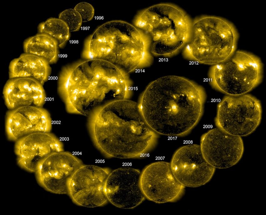
2                                                                                     Manuela Temmer

Contents

1  Introduction . . . . . . . . . . . . . . . . . . . . . . . . . . . . . .   .   .   .   .   .   .   .   .   .   .    2
2  Space Weather . . . . . . . . . . . . . . . . . . . . . . . . . . . .      .   .   .   .   .   .   .   .   .   .    7
3  Magnetic reconnection: common ground . . . . . . . . . . . . . .           .   .   .   .   .   .   .   .   .   .    8
4  Solar Flares . . . . . . . . . . . . . . . . . . . . . . . . . . . . . .   .   .   .   .   .   .   .   .   .   .   11
   4.1 Eruptive capability of an active region . . . . . . . . . . . .        .   .   .   .   .   .   .   .   .   .   11
   4.2 Eruptive solar flares: general characteristics . . . . . . . . .       .   .   .   .   .   .   .   .   .   .   13
5 Coronal mass ejections (CMEs) . . . . . . . . . . . . . . . . . . .         .   .   .   .   .   .   .   .   .   .   15
   5.1 General characteristics . . . . . . . . . . . . . . . . . . . . .      .   .   .   .   .   .   .   .   .   .   15
   5.2 CME early evolution . . . . . . . . . . . . . . . . . . . . . .        .   .   .   .   .   .   .   .   .   .   17
        5.2.1 Shock formation, radio bursts, and relation to SEPs             .   .   .   .   .   .   .   .   .   .   21
        5.2.2 Stealth CMEs . . . . . . . . . . . . . . . . . . . . . .        .   .   .   .   .   .   .   .   .   .   24
   5.3 Advantages due to multi-viewpoint observations . . . . . . .           .   .   .   .   .   .   .   .   .   .   25
6 Interplanetary counterparts of CMEs: ICMEs . . . . . . . . . . .            .   .   .   .   .   .   .   .   .   .   30
7 Solar Energetic Particles (SEPs) . . . . . . . . . . . . . . . . . .        .   .   .   .   .   .   .   .   .   .   34
   7.1 General characteristics . . . . . . . . . . . . . . . . . . . . .      .   .   .   .   .   .   .   .   .   .   34
   7.2 SEPs observed from multiple viewpoints . . . . . . . . . . .           .   .   .   .   .   .   .   .   .   .   37
8 Energy budget between flares, CMEs, and SEPs . . . . . . . . .              .   .   .   .   .   .   .   .   .   .   40
9 Structuring of interplanetary space: the solar wind . . . . . . . .         .   .   .   .   .   .   .   .   .   .   42
   9.1 General characteristics . . . . . . . . . . . . . . . . . . . . .      .   .   .   .   .   .   .   .   .   .   42
   9.2 Background solar wind . . . . . . . . . . . . . . . . . . . . .        .   .   .   .   .   .   .   .   .   .   48
   9.3 Solar wind structures affecting CME and SEP evolution . .              .   .   .   .   .   .   .   .   .   .   50
   9.4 Preconditioning of interplanetary space . . . . . . . . . . .          .   .   .   .   .   .   .   .   .   .   51
10 The chain of action on the example of the September 2017 events            .   .   .   .   .   .   .   .   .   .   52
11 Space weather forecasting models . . . . . . . . . . . . . . . . . .       .   .   .   .   .   .   .   .   .   .   57
12 Concluding remarks . . . . . . . . . . . . . . . . . . . . . . . . .       .   .   .   .   .   .   .   .   .   .   61

1 Introduction

Our Sun is an active star and as such undergoes cyclic variations, which are re-
lated to more or less frequently occurring activity phenomena observed at the
solar surface. High energetic activity phenomena, produced due to changes in
the Sun’s magnetic field, propagate through our solar system where they inter-
act with the planet’s atmospheres. At Earth, these interactions are well docu-
mented and known to cause geomagnetic disturbances having consequences for
modern society. The influence by the Sun on our solar system is termed Space
Weather. Therefore, solar activity needs to be permanently monitored from
space and ground in order to assess times of increased influence. International
space agencies created programs, such as ESA Space Situational Awareness
(SSA) or NASA Living with a star (LWS) (cf. Figure 1), to enhance Space
Weather awareness and with that support and fund on a long-term basis fun-
damental research and development of Space Weather forecasting tools.
    This review article focuses on the following Space Weather phenomena:
1.   Coronal mass ejections
2.   Flares
3.   Solar Energetic Particles
4.   Solar wind stream interaction regions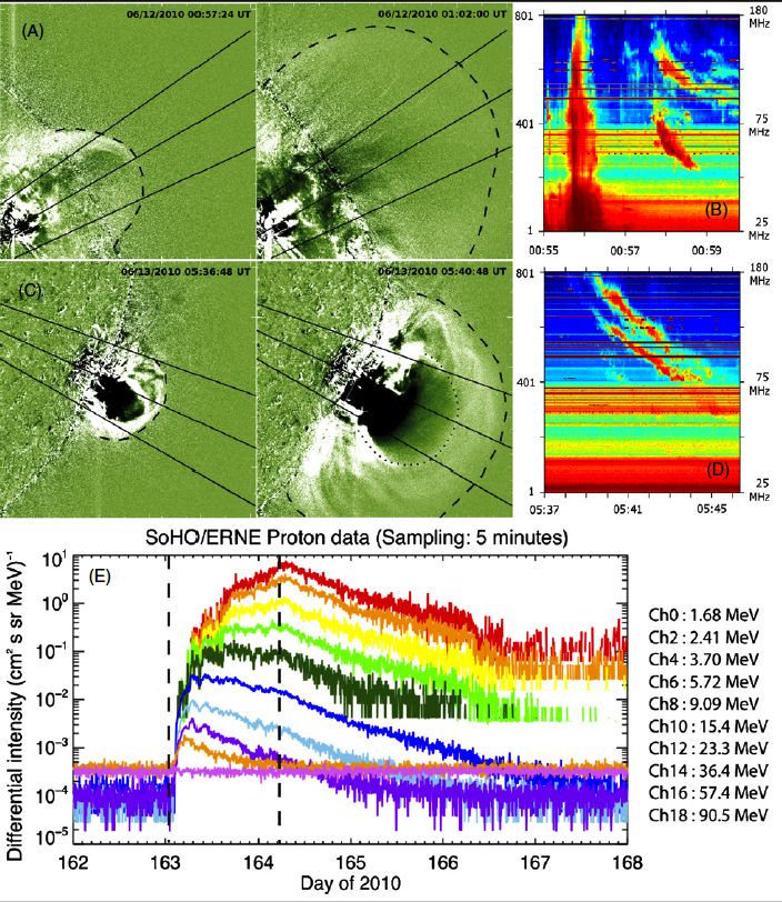
Space weather: the solar perspective                                                        3

Fig. 1 Solar activity phenomena (depicted here as CME) affect Earth and near-Earth space
and therefore, need to be permanently monitored. Space Weather forecasting is of global
interest and funded by international agencies. In the near future, satellites will observe the
Sun and its dynamic phenomena from different viewpoints, such as a combined L1 and L5
position. Image courtesy: ESA

    To properly describe these phenomena from the solar perspective, a number
of processes need to be understood, such as active region and magnetic field
evolution, energy build-up and release, as well as the global structuring of inner
heliospheric space. Space Weather is a topic of broad interest and sustains
an exciting and wealthy interdisciplinary research community1 . With that it
fosters information and knowledge exchange between international research
groups on solar-, heliospheric- and geo-space (Sun-to-impact disciplines) in
order to enhance scientific knowledge for improving existing and developing
new models for Space Weather forecasting.
    Coronal mass ejections (CMEs) are a rather recent phenomenon, discovered
just about 50 years ago, but in the meantime are known as the main drivers of
the most severe Space Weather disturbances (see e.g., Howard, 2006; Gopal-
swamy, 2016). They are huge structures that manifest themselves within some
tens of minutes as clouds of magnetized plasma impulsively expelled from the
Sun and subsequently propagating into interplanetary space (see e.g., Forbes,
2000). CMEs arise from usually complex and closed magnetic field structures
in equilibrium that is disrupted due to some instability causing its eruption
(e.g., emerging magnetic flux, remote reconfiguration of large scale magnetic
field, or field rotation; see e.g., Török et al., 2013; Schmieder et al., 2015; Green
  1 For example, the SCOSTEP effort that resulted in excellent publications via

CAWSES http://www.terrapub.co.jp/onlineproceedings/ste/CAWSES2007/index.html,
the VarSITI programs (e.g., ISEST Zhang et al., 2018, see http://www.varsiti.org) or the
international Space Weather Action Teams, iSWAT, where interdisciplinary groups gather
together under https://www.iswat-cospar.org.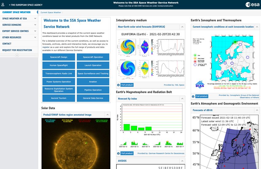
4                                                                 Manuela Temmer

et al., 2018). Instabilities in the solar magnetic field and their occurrence fre-
quency are modulated by the 11-year activity cycle of the Sun. The most
strong CME events may propagate the 1AU distance within a day (e.g., Cliver
et al., 1990; Gopalswamy et al., 2005a; Liu et al., 2014). Less strong events, on
average, propagate the same distance in up to 4 days (see e.g., Shanmugaraju
and Vršnak, 2014). CMEs may be linked to large geomagnetic disturbances,
due to shock compression and reconnection with the Earth’s magnetic field.
They may lead to ionospheric and geomagnetically-induced currents (see e.g.,
Pirjola et al., 2005). Usually the most severe geomagnetic storms are caused
by fast and massive CMEs, erupting from the central region of the visible solar
disk and carrying a strong southward magnetic field component that recon-
nects with the Earth’s magnetic field (see e.g., Pulkkinen, 2007). Consequently,
CMEs are a major topic of solar and Space Weather research.
    The power for making a CME energetic (i.e., being fast and wide) undoubt-
edly stems from the free magnetic energy which is released as consequence
of magnetic reconnection processes. Magnetic reconnection enables to impul-
sively drive plasma and to accelerate particles to high energies causing on the
one hand flare emission, which is observed in the solar atmosphere, and on
the other hand solar energetic particles (SEPs), which are measured in inter-
planetary space. Energetic particles from strong SEP events may reach almost
speed of light and travel the 1AU distance within about 10 minutes. High en-
ergy SEP events (about 1 GeV) may lead to enhanced proton fluxes even at
ground level. Hence, most intense events can endanger life and technology on
Earth and in space. Further consequences of CMEs and SEPs are disruptions
of satellite operations, radio communications and ground power systems (e.g.,
Bothmer et al., 2007). Unlike CMEs, having lead times of some tens of hours
between first observational signatures and impact at Earth, flares and SEP
events occur and impact almost simultaneously (see e.g., Lugaz et al., 2017b;
Cairns et al., 2018; Malandraki and Crosby, 2018). Accordingly, to predict the
occurrence of flares and SEPs one needs to predict the instabilities leading to
the onset of magnetic reconnection processes, one of the big challenges in solar
physics.
    The continuous solar wind flow in a quiet state (usually termed back-
ground solar wind) is represented by an alternation of slow and fast solar
wind streams that interact and form stream interaction regions (SIRs). If
steady in their existence and persisting over more than one solar rotation,
they are called co-rotating interaction regions (CIRs). During times of low
solar activity, Space Weather is dominated by CIR induced storms (Tsuru-
tani et al., 2006). Different flow speeds of the background solar wind also
change the propagation behavior of CMEs in interplanetary space. This has
consequences on the CME transit time and impact speed at planetary atmo-
spheres (drag force; see Gopalswamy et al., 2000; Vršnak, 2001; Cargill, 2004;
Vršnak, 2006). Moreover, CMEs disrupt the continuous outflow of the solar
wind and reconfigure the magnetic field on large spatial and short temporal
scales altering the background solar wind. For Space Weather and CME mod-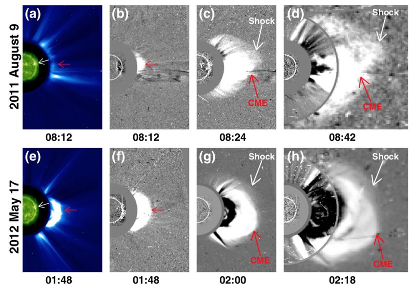
Space weather: the solar perspective                                                                 5

       Mars          Earth      L1       Venus                      Mercury             C3    Sun

                     215 Rs              155 Rs                      83 Rs              30 Rs 1 Rs
       320 Rs                  213 Rs

                    Hinode                        Solar Orbiter
                              ACE/Wind
                    Proba2
      MAVEN
      MAVEN                   /DSCOVR    VEX
                                                                  MESSENGER
                               SoHO/
                               STEREO
                                                                                        PSP

                                                                  BepiColombo
                     SDO
                    RHESSI
                     GOES                                               not to scale!

Fig. 2 Current and past space missions carrying instruments for gathering remote sensing
image data and in-situ plasma and magnetic field measurements. The majority of space-
craft is located in the ecliptic plane orbiting planets or at the Lagrangian point L1. The
coronagraph field of view of the SoHO/LASCO instrument C3 covers 30 solar radii. The
background white-light image is taken from STEREO/HI1+2 data covering about 90 degrees
in the ecliptic. Not to scale.

eling/forecasting purposes, these ever changing conditions in interplanetary
space are very challenging to tackle.
    For comprehensive investigations a rich source of observational data is cur-
rently available from many different instruments located at multiple viewpoints
and different radial distances (see Figure 2). In Earth orbit current operational
missions are e.g., GOES (Geostationary Operational Environmental Satellite),
SDO (SDO: Pesnell et al., 2012), Proba-2 (Santandrea et al., 2013), located at
L1 - 1.5 million km upstream of Earth - there is the Solar and Heliospheric Ob-
servatory (SoHO: Domingo et al., 1995), the Advanced Composition Explorer
(ACE: Stone et al., 1998), the WIND spacecraft Ogilvie et al. (1995), and
DSCOVR (Burt and Smith, 2012). At ∼1AU with variable longitudinal angles
from Earth, there is the Solar TErrestrial RElations Observatory (STEREO:
Kaiser et al., 2008) consisting of two identical spacecraft named STEREO-
Ahead and STEREO-Behind (lost signal end of 2014). The combination of
remote sensing image data and in-situ measurements is found to be optimal
for enhancing our knowledge about the physics of Space Weather phenomena.
For better understanding large eruptive activity phenomena, multi-viewpoint
and multi-wavelength data are exploited (e.g., combined L1, STEREO as well
as ground-based instruments). The various available data from spacecraft or-
biting around planets (e.g., VEX (2006–2014), MESSENGER (2011–2015),
MAVEN (2014–), BepiColombo (2018–)) also enable to analyze the evolution
of Space Weather phenomena as function of distance and longitude.
    A flagship of international collaboration and boost for Space Weather
research, is SoHO which now achieved 25 years in space. Figure 3 shows
SOHO/EIT (Delaboudinière et al., 1995) EUV image data covering the varia-
tions of the solar corona over a full magnetic solar cycle (Hale cycle). Long-term
observations are of utmost importance for monitoring and learning about the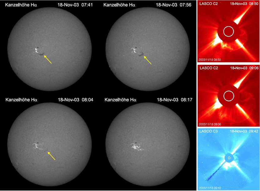
6                                                                          Manuela Temmer

Fig. 3 Each image shown here is a snapshot of the Sun taken every spring with the SOHO
Extreme ultraviolet Imaging Telescope (EIT) in the 284Å wavelength range. It shows the
variations of the solar activity in terms of increasing and decreasing number of bright active
regions visible in the corona. Courtesy: NASA/ESA

interaction processes of solar activity phenomena with Earth and other planets
as well as for improving our capabilities in Space Weather forecasting. Most
recent and unprecedented missions are Parker Solar Probe, launched in Au-
gust 2018 (Fox et al., 2016), and Solar Orbiter, launched in February 2020
(Müller et al., 2020) having on-board imaging and in-situ facilities with the
goal to approach the Sun as close as never before (∼0.05AU and ∼0.3AU)
and investigating the Sun out of the ecliptic (∼30 degrees). To support space
missions and for providing valuable complementary data, we must not forget
the importance of ground based observatories that observe the Sun over broad
wavelength and energy ranges allied in international networks such as the
Global high-resolution Hα network2 , the Global Oscillation Network Group3 ,
the database for high-resolution Neutron Monitor measurements4 , muon tele-

    2   http://bbso.njit.edu/Research/Halpha/
    3   https://gong.nso.edu
    4   E.g., http://www01.nmdb.eu/nest/search.php
Space weather: the solar perspective                                          7

scope networks, or the Worldwide Interplanetary Scintillation Stations Net-
work 5 .
    From the derived research results based on the observational data, over
the past years a plethora of models could be developed for predicting Space
Weather and their geomagnetic effects. The permanent monitoring of the Sun
and provision of data in almost real-time enabled to apply those results and
even to install operational services that produce forecasts mostly in an auto-
matic manner (e.g., facilitated by ESA/SSA6 ; NASA/CCMC7 ; NOAA/SWPC8 ).
However, the operational services also clearly demonstrated the limitations in
the forecasting accuracy as on average the errors are large and get worse with
increasing solar activity. This is mainly due to the large uncertainties com-
ing from the model input, namely observational parameters at or close to the
Sun. It also reveals the complexity of the interplay between the different driv-
ing agents of Space Weather, that makes it difficult to fully capture the physics
behind and to improve models. Reliable Space Weather forecasting is still in
its infancy.

2 Space Weather

From the historical perspective, the so-called “Carrington-event” from Septem-
ber 1, 1859 is the reference event for referring to extreme Space Weather and
with that the beginning of Space Weather research (see also Schwenn, 2006). At
that time only optical observations of the solar surface were performed and the
observed emitted radiation in white-light for that event showed impressively
the vast amount of energy that was distributed to the dense lower atmospheric
layers of the Sun where it heated the photosphere. At Earth, the associated ge-
omagnetic effects were observed in terms of aurora occurring from high to low
latitudes (e.g., Honolulu at 20 degrees northern latitude) and ground-induced
currents in telegraph wires (see Eastwood et al., 2017). The associated SEP
event is thought to be about twice as large as the huge SEP events from
July 1959, November 1960, or August 1972 (Cliver and Dietrich, 2013). Only
several years after the Carrington event, the usage of spectroscopes enabled
to regularly observe prominence eruptions revealing the dynamic changes of
the solar corona and material ejections with speeds exceeding hundreds of
km/s (Tandberg-Hanssen, 1995). The continuous monitoring of the Sun was
intensified in the 1940’s, when solar observations in radio, white-light and in
the Hα wavelength range were performed. At that time also galactic cosmic
rays were studied and found that they are anti-correlated with solar activity
(so-called Forbush decrease, measured as sudden drop in the cosmic ray flux
due to interplanetary disturbances; see also Cane, 2000). In the early 1960’s
 5   http://helios.mexart.unam.mx/pruebas/wipss/index.html
 6   http://swe.ssa.esa.int
 7   https://ccmc.gsfc.nasa.gov
 8   https://www.swpc.noaa.gov
8                                                                      Manuela Temmer

magnetic structures driving shocks were inferred from observations in the met-
ric radio observations and geomagnetic storm sudden commencements (Gold,
1962; Fokker, 1963). The transient events with mass moving through the solar
corona and actually leaving the Sun, i.e., CMEs, that were associated with the
prominence/filament eruptions were discovered only in the early 1970’s with
the advent of the space era (see Tousey, 1971; MacQueen et al., 1974). Recent
reviews on the history of prominences and their role in Space Weather can be
found in (Vial and Engvold, 2015; Gopalswamy, 2016, and references therein).
While most of the extreme space weather events happen during the solar cycle
maximum phase, occasionally strong geoeffective events may occur close to
the solar cycle minima and also during weak solar activity, provided there are
appropriate source regions on the Sun (see also e.g., Vennerstrom et al., 2016;
Hayakawa et al., 2020). For more details about the solar cycle see the Living
Reviews by Hathaway (2010).
    Nowadays, a wealth of space and ground-based instruments are available,
delivering valuable observational data, as well as modeling facilities. This en-
ables to study in rich detail the manifold processes related to Space Weather
events and to better understand the physics behind. To forecast the geomag-
netic effects of an impacting disturbance at Earth (e.g., by the Dst9 or Kp
index10 ), the most common parameters we need to know in advance - and
various combinations of these - are the amplitude/orientation and variation of
the north-south component of the interplanetary magnetic field (Bz ), speed
(v), and density (n). Especially, the electric field vBs (Bs = Bz < 0) is found
to show a high correlation with the Dst storm index (see e.g., Baker et al.,
1981; Wu and Lepping, 2002; Gopalswamy et al., 2008a). For details on the
geomagnetic effects of Space Weather phenomena as described here, see the
Living Reviews by Pulkkinen (2007).
    The Space Weather “chain of action” from the solar perspective is described
best by the recent example of the multiple Space Weather events that occurred
in September 2017 (see Section 10). But before that, we elaborate the physical
basis.

3 Magnetic reconnection: common ground

The commonality that unites everything and yet produces such different dy-
namic phenomena is magnetic reconnection and the release of free magnetic
energy. This leads to particle acceleration, heating, waves, etc. and to a re-
structuring of the (local) magnetic field in the corona by newly connecting
different magnetic regimes and with that changing magnetic pressure gradi-
ents. Especially the latter shows to affect the solar corona globally.
  9 The disturbance storm time (Dst) index monitors variations in the Earth’s equatorial

ring current.
 10 The planetary K index (Kp) monitors variations in the horizontal component of the

Earth’s magnetic field.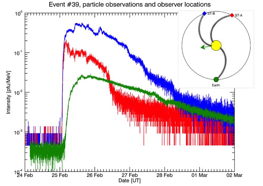
Space weather: the solar perspective                                                                                          9

        ambient solar wind

                              . .
                                                .. .
                                                ..
                                .. . .
                             . .. . .
                                  .

                                             flux rope
                                                CME
                                 flux rope
                                   CME

                                                                                                H! ribbons
                                                                          Post-eruptive loops
                                                                             (SXR, EUV)
                                                    Post-eruptive loops
                                                       (SXR, EUV)

                                                                                                             (HXR emission)
 SEPs

Fig. 4 Left: Stochastic acceleration model for solar flares. Magnetic field lines (green) and
turbulent plasma or plasma waves (red circles) generated during magnetic reconnection. Blue
arrows and areas mark accelerated particles impinging on the lower denser chromosphere
where they produce Bremsstrahlung and on the upside may escape to interplanetary space
where they are detected as SEPs (adapted from Petrosian and Liu, 2004; Vlahos et al.,
2019). Middle: CME-flux rope configuration in the classical scenario (CSHKP) covering also
the post eruptive arcade usually observed in SXR and EUV wavelength range (adapted from
Lin and Forbes, 2000); Right: CME flux rope acting as driver of a bow shock (black arc) may
accelerate SEPs (black dots) in the corona or heliosphere via diffusive shock acceleration
(adapted from Mikić and Lee, 2006).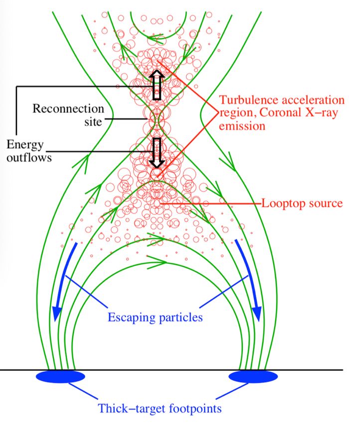
10                                                               Manuela Temmer

    In order to derive a complete picture about Space Weather, we first need to
understand the interrelation between these many individual processes start-
ing at the Sun. This covers a cascade of small and large scale phenomena
varying over different time scales. The primary source of Space Weather pro-
ducing phenomena, i.e., CMEs-flares-SEPs (note that in the following eruptive
phenomena are considered and not stealth CMEs), are active regions repre-
senting the centers of strong magnetic field and energy (more details on the
evolution of active regions, see the Living Reviews by van Driel-Gesztelyi and
Green, 2015; Toriumi and Wang, 2019). However, in detail the energy build-
up and release processes are not well understood. The key-driver certainly is
the magnetic field configuration below the visible surface (photosphere), that
cannot be directly observed and characterized for giving reliable predictions
of its status and further development. The lack of magnetic field information
is also given in the upper atmospheric layers. There are currently no instru-
ments enabling measurements of the magnetic field in the corona, hence, we
need to rely on models simulating the coronal and, further out, interplanetary
magnetic field (see, e.g., the Living Reviews by Gombosi et al., 2018, on coro-
nal and solar wind MHD modeling ). While active regions are characterized
by closed magnetic field, coronal holes cover mainly open magnetic field from
which high speed solar wind streams emerge. They structure interplanetary
space and set the coupling processes between continuous solar wind flow and
transient events. To better understand the propagation behavior of transient
events, we also need to study the evolution and characteristics of the solar
wind flow, and hence, the interplay between open and closed magnetic field.

    Figure 4 sketches three different time steps in the evolution of an eruptive
flare event, causing a CME and SEPs, as a consequence of magnetic recon-
nection (see Petrosian and Liu, 2004; Lin and Forbes, 2000; Mikić and Lee,
2006). The left panel of Figure 4 focuses on the early evolution stage of the
eruptive event, introducing stochastic acceleration processes causing high ener-
getic particles to precipitate along magnetic field lines towards and away from
the Sun. Flare emission is observed on the solar surface due to the acceleration
of particles towards the Sun. Particles that escape into interplanetary space
along the newly opened magnetic field, produce SEPs. The middle panel of
Figure 4 shows the creation of the CME body, i.e., the production of a closed
magnetic field structure (flux rope), as well as the related post-eruptive arcade
which is formed below. The exact acceleration mechanism(s) of SEPs is still
an open issue, hence, cartoons as shown here usually present both possible
driving agents, the flare and the CME shock. To complete the picture for a
flare-CME-SEP event, the right panel of Figure 4 depicts the interplanetary
magnetic field and its behavior which differs from the typical Parker spiral
orientation due to the propagating CME shock component causing SEP accel-
eration in interplanetary space. The deviation of the interplanetary magnetic
field from the nominal Parker spiral is an important issue when dealing with
magnetic connectivity for studying SEPs and propagation behavior of CMEs.
Space weather: the solar perspective 11
In the following, we will discuss in more detail the characteristics of the
different manifestations occurring in an eruptive flare event.
4 Solar Flares
4.1 Eruptive capability of an active region
Active regions may be classified either by the morphology of an active region
using the McIntosh classification (McIntosh, 1990) or the magnetic structure
using Hale’s/Künzel’s classification (Künzel, 1960). Due to the emergence of
magnetic flux the degree of complexity in the magnetic field of an active re-
gion grows, which increases the likeliness to create strong flares and CMEs
(e.g., Sammis et al., 2000; Toriumi et al., 2017). The probability that an X-
class flare is related to a CME is found to be larger than 80% (Yashiro et al.,
2006), however, there are well observed exceptions reported. So-called con-
fined flares are neither accompanied by a CME nor a filament eruption (e.g.,
Moore et al., 2001). Their special magnetic field configuration allows particle
acceleration (observed as flare), but they do not escape into interplanetary
space and, hence, do not produce SEPs (Gopalswamy et al., 2009). Therefore,
confined flares may produce strong X-ray emission but, presumably due to a
strong bipolar overlying coronal magnetic field configuration, are not related
to the opening of the large-scale magnetic field (e.g., Wang and Zhang, 2007;
Sun et al., 2015; Thalmann et al., 2015). The electromagnetic radiation of con-
fined flares can still instantaneously cause sudden changes in the ionospheric
electron density profile (disturbing radio wave communication or navigation),
also known as solar flare effect or geomagnetic crochets (Campbell, 2003) but
occurring rather rarely. However, confined flares are also potential candidates
for false Space Weather alerts in terms of an erroneous forecast of geomagnetic
effects due to the magnetic ejecta that would have arrived tens of hours later
at Earth.
Therefore, the manifestation of the eruptive capability of an active region
is one of the prime targets for prospective forecasting of SEPs and CMEs.
For example, the length of the main polarity inversion line of an active region
or the magnetic shear and its sigmoidal morphology, is obtained to be highly
indicative of the potential to open large scale magnetic field and to produce
CMEs and SEPs (e.g., Canfield et al., 1999). Studies also showed that active
regions, for which the polarity inversion line quickly changes with height into
a potential field configuration, are more favorable for producing non-eruptive
events (Baumgartner et al., 2018). Likewise, the decay index of the horizontal
magnetic field (ratio of the magnetic flux in the lower corona to that in the
higher corona) is found to be lower for failed eruptions compared to that for
full eruptions (cf., Török and Kliem, 2005; Fan and Gibson, 2007; Guo et al.,
2010; Olmedo and Zhang, 2010).12 Manuela Temmer Fig. 5 Flare-CME-SEP relation in time. The onset of the solar flare is indicated by the vertical red line. The grey shaded area marks the time difference between flare start and SEP flux increase for MeV energies. Taken from Anastasiadis et al. (2019) who adapted it from Miroshnichenko (2003). For more details on the issue of flare-productive active regions I refer to the Living reviews by Toriumi and Wang (2019). See also Forbes (2000), Webb and Howard (2012), Parenti (2014), or Chen (2017) for a more theoretical approach on that issue.
Space weather: the solar perspective                                                  13

4.2 Eruptive solar flares: general characteristics

Flares are observed to release a huge amount of energy from 1019 up to 1032
erg over a timescale of hours11 . With the advent of modern ground-based and
space-borne instruments, our small optical window was massively enlarged and
it is now well-known that this energy is radiated over the entire electromagnetic
spectrum from decameter radio waves to gamma-rays beyond 1 GeV. Figure 5
depicts the temporal relation between flare emission, observed in different
wavelength ranges, CME kinematics and SEP flux profiles in the GeV and MeV
energy range. The flare activity profile consists of a so-called pre-flare phase,
showing thermal emission in SXR and EUV, as well as Hα kernel brightenings.
If related to a filament eruption, this phase partly coincides with the slow rise
phase of the filament12 . This is followed by the impulsive flare phase during
which most of the energy is released and non-thermal emission in terms of
hard X-ray (HXR) footpoints appears due to particles accelerating out of the
localized reconnection area and bombarding the denser chromosphere where
they emit Bremsstrahlung (for a review on solar flare observations see e.g.,
Fletcher et al., 2011). At this point also the CME body forms as consequence
of the closing of the magnetic field lines in the upper part of the reconnection
area revealing a flux rope structure (note that the most compelling argument
for an already existing flux rope is actually a filament). As the flare emission
increases also the SEP flux in the GeV energy range starts to rise. After
the flare reaches a maximum in intensity, the decay phase is observed during
which the intensity level goes back to the background level from before the
flare start. The exact timing of the rise and decay phase is dependent on the
energy release and the energy range in which the flare is observed which is
known as the so-called Neupert effect (the HXR flux rise phase time profile
corresponds to the derivative of the SXR flux time profile; see Neupert, 1968).
The last phase may have a duration of several hours or longer. During that
phase also post-eruptive arcades (or loops) start to form, that may still grow
over 2–20 hours. The growth of the post-eruptive arcade is hinting towards
an ongoing reconnecting process, which is not energetic enough to produce a
significant emission in EUV or SXR (see e.g., Tripathi et al., 2004). For more
details on the global properties of solar flares I refer to the review by Hudson
(2011).
     Figure 6 shows the temporal evolution of a flare and erupting filament
observed in Hα and the associated CME observed in white-light coronagraph
image data. The event is classified in the emitted SXR flux as GOES M3.9 flare
(corresponding to the measured power of 3.6×10⁻⁵ W/m2 ) which occurred on
November 18, 2003 in a magnetically complex βγ active region. The associated
CME caused two days later one of the strongest geomagnetic storms of solar
cycle 23 having a minimum Dst value of −472 nT (Gopalswamy et al., 2005b).
 11 An automatically updated list of flares is available under http://www.lmsal.com/

solarsoft/latest_events/ or https://www.solarmonitor.org
 12 Filament detection and eruption catalogues can be found e.g., under http://cesar.kso.

ac.at/sn_iv/filaments.php or http://aia.cfa.harvard.edu/filament/
14 Manuela Temmer
Fig. 6 Global flare evolution and relation to CME from the November 18, 2003 event. Left
panels: Hα filtergrams from the Kanzelhöhe Solar Observatory (Austria). The associated
erupting filament is indicated by arrows. Right panels: Temporal evolution of the CME in
coronagraph images from SOHO/LASCO. Taken from Möstl et al. (2008).
Inspecting the time stamps on the image data of that event, about one hour
after the appearance of the flare signatures, the CME became visible in the
coronagraph. The filament started to rise some tens of minutes before the flare
emission occurred.
The orientation of the magnetic structure, especially of the Bz component,
of an ICME is key to forecast its geoeffectiveness and poses the Holy Grail of
Space Weather research. Knowing the flux rope orientation already at the Sun
could provide information on the impact of CMEs early in advance, hence, as
soon as they erupt or even before. While the handedness of flux ropes can be
well observed from in-situ measurements (Bothmer and Schwenn, 1998; Mul-
ligan et al., 1998), on the Sun observational proxies need to be used. Figure 7
shows several surface signatures from which the magnetic helicity (sense of
twist of the flux rope: right-handed or left-handed) can be inferred. Typically,
in EUV observations these are sigmoidal structures (S- or reverse S-shaped) or
post-eruptive arcades (skewness of EUV loops and polarity of the underlying
magnetic field), in Hα the fine structures of filaments are used (orientations
of barbs) or statistical relations like the hemispheric helicity rule (see Wang,
2013). However, strong coronal channeling, latitudinal and also longitudinal
deflection and/or rotation, that the magnetic component of the CME under-
goes as it evolves through the low solar corona, may change those parameters asSpace weather: the solar perspective 15
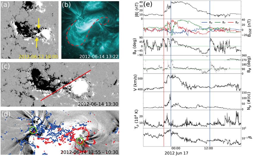
(e)
left-handed
right-handed
Fig. 7 (a) SDO/HMI data from June 14, 2012 showing the magnetic tongues of the erupting
active region revealing a positive chirality. (b) Forward-S sigmoidal structure from the coro-
nal loops observed by SDO/AIA 131Å, indicating a right-handed flux rope. (c) SDO/HMI
magnetogram showing the approximated polarity inversion line (red line). (d) Base-difference
SDO/AIA 131Å image overlaid with the HMI magnetogram contours saturated at ±200 G
(blue = negative polarity; red = positive polarity). The dimming regions indicating the flux
rope footpoints are marked by green circles. Panels (a–d) are adapted from Palmerio et al.
(2018). (e) The cartoon shows the handedness inferred from the magnetic field and sigmoidal
structures or orientation of post eruptive loops.
shown in various studies by e.g., Shen et al. (2011); Gui et al. (2011); Bosman
et al. (2012); Panasenco et al. (2013); Wang et al. (2014); Kay and Opher
(2015); Möstl et al. (2015), or Heinemann et al. (2019). Recent approaches in
ICME Bz forecasting can be found in, e.g., Savani et al. (2015), Palmerio et al.
(2017), or Kay and Gopalswamy (2017).
For more details about the energetics and dynamics of solar flares I refer
to the Living Reviews by Benz (2017) and for the magnetohydrodynamic pro-
cesses in active regions responsible for producing a flare to the Living Reviews
by Shibata and Magara (2011).
5 Coronal mass ejections (CMEs)
5.1 General characteristics
CMEs are optically thin large-scale objects, that quickly expand, and are tra-
ditionally observed in white-light as enhanced intensity structures. The inten-16 Manuela Temmer
sity increase is due to photospheric light that is Thomson scattered off the
electrons forming the CME body and integrated over the line-of-sight (Hund-
hausen, 1993). Due to strong projection effects their apparent morphology
greatly depends on the viewpoint and, hence, makes CMEs a rather tricky
object to measure (see e.g., Burkepile et al., 2004; Cremades and Bothmer,
2004).
By using coronagraphs, CMEs are visible with teardrop-like shapes that are
characterized by multiple structures. Figure 8 shows SOHO/LASCO (Brueck-
ner et al., 1995) coronagraph white-light images of two CMEs having different
propagation directions. For the CME that leaves the Sun in a rather perpen-
dicular angle to the observer (left panel of Figure 8), the various CME struc-
tures are well visible. In general, we distinguish between the shock (yellow
arrow) and CME body (green arrow) that are followed by some cavity created
by the expanding magnetic flux rope (red arrow) and an increased bright-
ness structure (orange arrow). Partly these structures are detected also from
in-situ measurements for the interplanetary counterparts of CMEs (ICMEs;
see Section 6). The increased brightness structure consists of prominence ma-
terial (Vourlidas et al., 2013) or is suggested to appear due to a brightness
increase of the two overlapping CME flanks (Howard et al., 2017). The sheath
region behind the shock has less clear signatures in coronagraph images taken
close to the Sun as it is generated later when the solar wind plasma gets
piled-up in interplanetary space (see e.g., Kilpua et al., 2017; Salman et al.,
2020). For CMEs propagating in the line-of-sight towards or away from the
observer (right panel of Figure 8), the different structures are less well visible.
As these CMEs are launched close to the central meridian of the observed disk,
they most severely suffer from projection effects. Energetic ones are frequently
observed as so-called halo CMEs, revealing extensive white-light signatures
made of compressed plasma material surrounding the occulting disk of a coro-
nagraph. For halo CMEs, evidence that the CME is actually moving towards
the observer is given from the associated activities observed on the solar disk
(such as filament eruptions, flare emission, dimming regions, or coronal wave
signatures). Highly relevant for Space Weather, halo CMEs are of special in-
terest and are diversely studied mostly by using single spacecraft data from
the coronagraphs aboard SoHO.
Up to the distance of about 30 solar radii (LASCO/C3 field of view), sta-
tistical studies showed that CMEs undergo several phases in their dynamics.
Before the actual launch a slow rising phase occurs (initiation phase), contin-
ued by the acceleration phase over which a rapid increase in speed is observed
in the inner corona, that is followed by a rather smooth propagation phase
as the CME leaves the Sun (Zhang and Dere, 2006). On average, over the
coronagraphic field of view, CME fronts reveal radial speeds in the range of
300–500 km/s with maximum values observed up to 3000 km/s, accelerations
of the order of 0.1–10 km/s2 , angular widths of about 30–65 degrees and masses
of ∼1014 –1016 g (e.g., Vourlidas et al., 2010; Lamy et al., 2019). The ratio in
density between the CME body and surrounding solar wind decreases from
∼11 at a distance of 15 solar radii to ∼6 at 30 solar radii (Temmer et al.,Space weather: the solar perspective 17 Fig. 8 LASCO CME excess mass images showing the expanding shock wave front (yellow arrow) and the CME leading edge density enhancement (green arrow) for two different events. For the CME propagating rather in the plane of sky (left panel), typical structures such as the cavity due to the expanding magnetic ejecta (red arrow) followed by some intensity enhancement (orange arrow) can be observed, that is less well visible for the halo CME (right panel). The projected LASCO CME speeds are given in the legend (adapted from Vourlidas et al., 2013). 2021). However, CMEs vary in their occurrence rate as well as in their char- acteristics over different solar cycles. While flare rates and their properties have not changed much over the past solar cycles, the CME properties for solar cycle 24 are significantly different as given in recent statistics (Lamy et al., 2019; Dagnew et al., 2020b). CMEs were found to be more numerous and wide compared to solar cycle 23. Close to the Sun, the CME expansion is driven by the increased magnetic pressure inside the flux rope, while further out they most probably expand due to the decrease of the solar-wind dynamic pressure over distance (Lugaz et al., 2020). Therefore, the increased width for CMEs of cycle 24 may be explained by the severe drop (∼50% ) in the total (magnetic and plasma) heliospheric pressure (see e.g., McComas et al., 2013; Gopalswamy et al., 2014, 2015; Dagnew et al., 2020a). Interestingly, also the maximum sunspot relative number in cycle 24 reached only 65% of that from cycle 2313 . The different expansion behaviors have consequences also for Space Weather effects in terms of their abilities in driving shocks (see e.g., Lugaz et al., 2017a). 5.2 CME early evolution Besides the traditional observations in white-light images, also EUV or SXR imagery reveal CME signatures, presumably due to compression and heating 13 http://sidc.be/silso/cyclesminmax
18                                                                       Manuela Temmer

Fig. 9 STEREO-B observations of the CME from August 24, 2014. The images show
combined EUVI (304Å) and COR1 image data. Filament plasma material is ejected into
space forming the bright CME core following the cavity. Plasma that is lacking sufficient
kinetic energy to escape from the Sun’s gravity, falls back onto the solar surface. Credit:
STEREO/NASA. The movie is online available.

that makes it visible in filtergrams sensible for high temperatures (see e.g.,
Glesener et al., 2013). Satellite missions that carry EUV instruments having
large field of views can be effectively used with combined white-light corona-
graph data to track CME structures for deriving the kinematical profile over
their early evolution covering the CME main acceleration phase. The SEC-
CHI instrument suite (Howard et al., 2008) aboard STEREO provides EUV
and white-light data that seamlessly overlap14 . as shown in Figure 9. For such
studies one needs to keep in mind that the observational data image different
physical quantities (density and temperature in EUV, and density in white-
light), hence, dark and bright features in both image data do not necessarily
match.
    From combined high temporal resolution EUV and white-light data a more
detailed understanding about the energy budget (see also Section 8) and rela-
tion between flares, filaments and CMEs is revealed providing relevant informa-
tion for SEP acceleration and generation of radio type II bursts. It is found that

 14 SoHO EIT and C1 also provided that possibility but C1 was lost in June 1998 due to

spacecraft failure. For a couple of events the usage of combined EIT-C1 data could be shown
(see Gopalswamy and Thompson, 2000; Zhang et al., 2001; Cliver et al., 2004b).
Space weather: the solar perspective 19
the thermal flare emission observed in SXR and the CME speed profile show
similar behavior in timing (Zhang et al., 2001, 2004; Chen and Krall, 2003;
Maričić et al., 2007). For strong eruptive events an almost synchronized behav-
ior between flare HXR emission and CME acceleration is obtained through a
feedback relation (Temmer et al., 2008, 2010). The CME acceleration is found
to peak already as low as about 0.5 solar radii above the solar surface (for
statistics see Bein et al., 2011). Figure 10 gives the schematic profiles and dis-
tances over time between non-thermal (HXR) and thermal (SXR) flare energy
release and CME kinematics (acceleration, speed). The flare-CME feedback
loop can be well explained by the CSHKP standard model (Carmichael, 1964;
Sturrock, 1966; Hirayama, 1974; Kopp and Pneuman, 1976) through the mag-
netic reconnection process underlying both activity phenomena. In a simplistic
scenario, we may summarize that magnetic reconnection drives particle accel-
eration (neglecting details on the actual acceleration process) leading to flare
emission and closes magnetic field increasing the magnetic pressure inside the
presumable CME flux rope (neglecting details on the actual magnetic configu-
ration of the active region and surrounding). For strong flares that are related
to CMEs of high acceleration values, the available free magnetic energy might
be larger. This occurs preferably for CMEs initiated at lower heights where
the magnetic field is stronger. With that, particles get accelerated to larger
energies, hence, producing stronger flares, and more poloidal flux can be added
per unit time, hence, generating a stronger expansion of the flux rope and a
faster CME eruption. This is supported by theoretical investigations on the
feedback process, covering magnetic reconnection with the ambient coronal
magnetic field (reconnective instability Welsch, 2018). More details are found
in, e.g., Chen and Krall (2003); Vršnak et al. (2007); Vršnak (2008); Jang et al.
(2017).
Associated to the erupting CME, we frequently observe coronal dimming
regions that evolve over a few tens of minutes (Hudson et al., 1996; Webb
et al., 2000). Core dimming regions are assumed to be located at the anchoring
footpoints of the associated magnetic flux rope and reveal the loss of plasma
from the corona into the CME structure adding mass to the CME body (see
Temmer et al., 2017b). Secondary dimming regions most probably refer to
mass depletion in the wake of the large-scale magnetic field opening as the
CME fully erupts (for more details on core and secondary dimming regions,
see Mandrini et al., 2007). Recent studies discovered a strong relation between
dimming intensity and flare reconnected flux as well CME speed (e.g., Dissauer
et al., 2018, 2019). Also the final width of the CME can be estimated from the
amount of magnetic flux covered by the CME associated post-eruptive flare
arcade as the surrounding magnetic field prevents the CME flux rope from
further expansion (Moore et al., 2007). On the contrary, the CME surrounding
shock as well as associated coronal waves on the solar surface, that are ignited
by the lateral CME expansion, are freely propagating and are not limited in
their spatial extend (for more details on globally propagating coronal waves I
refer to the Living Reviews by Warmuth, 2015).20 Manuela Temmer
b)
CME acceleration
Flare SXR flux
Flare HXR flux
CME velocity
Distance
Propagation phase
Time
> 2Rs
Acceleration phase
(20-30min)
< 0.5Rs
a)
CME dynamic evolution
Fig. 10 CME-flare relation. a) schematics of the thermal (SXR) and non-thermal (HXR)
flare energy release in comparison to the CME kinematical evolution close to the Sun. It is
found that CME acceleration and HXR emission as well as the CME speed and SXR emis-
sion, respectively, are closely related. Taken from Temmer (2016). b) observational results
for the December 22, 2009 CME event revealing the early evolution from combined EUV
and coronagraph data (STEREO-B spacecraft) and GOES SXR flux profile for the related
flare and derivative (proxy for HXR emission). Taken from Bein et al. (2012).Space weather: the solar perspective 21
To derive in more detail the temporal linking of flare-CME-SEP events,
image data covering large field of views for observing the lower and middle
corona is of utmost importance. Figure 11 shows the different field of views
of currently available and future EUV instruments to observe and study the
middle corona (distance up to about 4 solar radii). The Extreme EUV Imager
suite aboard Solar Orbiter works at the 174Å and 304Å EUV passbands (EUI:
Rochus et al., 2020). The EUVI-LGR instrument aboard ESA’s Lagrange L5
mission (launch planned for 2027) has an extended field of view to the West
limb of the Sun, that is perfectly suited to track the early evolution of Earth
directed CMEs from L5 view (60 degrees separation with Earth). We must
not forget the capabilities of ground-based coronagraph instruments such as
the COSMO K-Cor at the Mauna Loa Solar Observatory in Hawaii (replaced
in 2013 the aging MLSO Mk4 K-coronameter15 ) observing a field of view
starting as low as 1.15 solar radii, however, quite restricted in observational
time compared to satellite data.
For more details on CME trigger mechanisms I refer to recent review ar-
ticles by Schmieder et al. (2015) or Green et al. (2018). For a more specific
background on CME initiation models, see, e.g., the Living Reviews by Webb
and Howard (2012).
5.2.1 Shock formation, radio bursts, and relation to SEPs
Closely related to studies of the CME early evolution and acceleration profiles,
are shock formation processes. To generate a shock wave, a short-duration
pulse of pressure is needed. Besides the CME, acting as piston, there is also
the possibility that a strong flare energy release initiates a blast wave or simple-
wave shock (e.g., Vršnak and Cliver, 2008). At which height shocks are formed
by an erupting disturbance is important for understanding particle acceleration
processes. The acceleration profile derived from tracking the CME frontal part
suggests its formation at rather low coronal heights22 Manuela Temmer Fig. 11 EUV image from Proba-2/SWAP combined with a LASCO/C2 coronagraph image covering in total a field of view up to ∼4 solar radii. The colored boxes mark the relative nominal field of views of different EUV observing instruments. FSI (Full Sun Imager is part of the EUI suite aboard Solar Orbiter), EUVI-LGR (aboard the planned L5 Lagrange mission), and SoHO/EIT. STEREO/EUVI, Proba-2/SWAP, GOES/SUVI are instruments with the largest field of view of about 1.7 solar radii. Taken from http://middlecorona.com. 2018). Due to the large density in the lower coronal heights a large compression appears with a quasi-perpendicular geometry, favoring the shock formation process. In that respect, moving type IV radio bursts might actually represent shock signatures due to CME flank expansion, that can be used as additional diagnostics for studying the lateral evolution of a CME (Morosan et al., 2020). The SEP intensity is found to be correlated with the width of a CME, and as such identifies the CME flank region to be an efficient accelerator of particles (see Holman and Pesses, 1983; Mann and Klassen, 2005; Richardson et al., 2015). Comparing the CME apex and flanks, the field lines are disturbed at different heights that may lead to different onset times for the acceleration of SEPs (cf., Figure 20). The time needed for shock formation also leads to a temporal delay of the onset of SEP events with respect to both, the initial energy release (flare) and the onset of the solar type II radio burst (evidence of shock formation). Hence, the timing is an important factor and has to be taken into account when relating these phenomena to each other.
Space weather: the solar perspective                                                      23

                                                                Type III
                                                                            Type II

                                                                        Type II

Fig. 12 Two CME events and associated coronal waves (June 12 and 13, 2010) are investi-
gated with high cadence SDO EUV 211Å data. Manually tracked positions of the wavefronts
are marked by dashed black lines. The connection between coronal surface wave and CME
front is nicely observed. The right panels give radio data (Learmonth observatory, Australia)
revealing type III and type II bursts (upper and lower frequency band) and measurements
from particle detectors at L1 (bottom panel; vertical dashed lines show AIA waves onsets).
Adapted from Kozarev et al. (2011).

    Shocks may also be formed at larger distances from the Sun (several tens
of solar radii), depending on the acceleration phase duration, the maximum
expansion velocity and the width of the CME (Žic et al., 2008). Due to the de-
clining magnetic field with distance (well defined band-splits in type II bursts
can be used to estimate the magnetic field in the corona; see e.g., Vršnak et al.,
2002), shocks forming at larger heights are related to softer SEP spectra (e.g.,
24 Manuela Temmer
Gopalswamy et al., 2017a). As can be seen, CME acceleration, shock formation
height and hardness of SEP spectra is closely connected. Compared to SEPs,
which strongly depend on the magnetic connectivity with the observer, type
II bursts can be observed without connectivity issues and thus, give additional
information about particle acceleration processes driven by CME shocks. In
that respect, type II radio bursts may be used for predicting SEPs as well as
shock arrival times (e.g., Gopalswamy et al., 2008b; Cremades et al., 2015).
In combination, these parameters have strong implications for Space Weather
impact, revealing the importance of monitoring and studying the early evolu-
tion phase of solar eruptive events. More details on SEPs are given in Section
7.
Figure 12 presents a case study about the evolution of a CME front close to
the Sun by using high cadence EUV images from SDO for June 12 and 13, 2010.
The derived kinematics of the CME reveals a fast acceleration of its frontal
part with about 1 km/s2 over the distance range 1.1–2.0 solar radii. The almost
vertical traces in the radio spectra are type III bursts, identified with streams
of electrons (radio emission due to particles moving along open magnetic field
lines), followed by diagonal structures of a moving type II bursts, identified
with shock waves. The onset of the type II burst appears together with the
CME shock front, as observed in EUV, with a bit of a delay with respect to the
shock formation that occurs close to the maximum CME acceleration. By the
time the CME occurs in the LASCO field of view, the CME speed decreased to
the sub-Alfvénic regime. The event produced an enhanced proton flux at 1AU.
However, the complex magnetic topology related to the active region prevents
from making strong conclusions about the possible sites of particle acceleration
(see also Kozarev et al., 2011; Ma et al., 2011; Gopalswamy et al., 2012).
Definitely, more such detailed case studies combined with improved modeling
of the magnetic environment is needed for advancing our understanding in the
processes that accelerate particles.
5.2.2 Stealth CMEs
In contrast to fast and massive CMEs and their related cascade of solar surface
signatures, there exist so-called stealth CME events that are most probably
caused by some simple (low-energetic) magnetic field reconfiguration in the
upper corona releasing magnetic flux ropes of low density that usually do not
exceed the solar wind flow speed. Actually, they were recognized already in the
mid 1980’s and were identified as spontaneous CMEs or unassociated CMEs
(meaning no surface signatures) by Wagner and Wagner (1984). Later studies
showed, that they start at very large heights in the corona without noticeable
signatures, such as flare emission, filament eruptions, coronal waves, or coronal
dimmings (Robbrecht et al., 2009). Stealth CMEs are potential candidates to
cause problem storms and missed Space Weather events, as they are hardly
recognized in white-light data and due to the lack of observational imprints on
the solar disk. In the recent years several studies have been published on thisSpace weather: the solar perspective 25
B A
Fig. 13 Earth-directed CME from December 12, 2008 as observed from multiple perspec-
tives. STEREO-A (left) and STEREO-B (right) are separated from Earth by an angle of
about 45 degrees. The running difference image from LASCO/C2 (middle panel) observes
the CME as weak partial halo event. The inlay in the middle panel gives the spacecraft
location (STEREO-A red filled circle; STEREO-B blue filled circle) with respect to Earth
(green filled circle) and the CME propagation direction (yellow arrow). White arrows in each
panel point to roughly similar parts of the CME observed with the different instruments.
The closer the CME propagates in the plane-of-sky of the instrument, the higher the intensity
in white-light. Adapted from Byrne et al. (2010).
issue discussing those events (see e.g., D’Huys et al., 2014; Nitta and Mulligan,
2017; Vourlidas and Webb, 2018).
5.3 Advantages due to multi-viewpoint observations
In contrast to a flare, which is a rather localized phenomenon, the analyzes of
CMEs and related coronal waves, propagating over large areas of the solar sur-
face, as well as SEPs profit enormously from at least two viewpoints. The twin-
spacecraft STEREO unprecedentedly provides, since its launch end of 2006,
image data in EUV and white-light from multiple perspectives. STEREO con-
sists of two identical spacecraft, STEREO Ahead (A) and Behind (B; lost
signal October 2014), orbiting the Sun in a distance close to Earth, with
STEREO-A being closer and STEREO-B further away from the Sun. The
separation angle between the two spacecraft increases by about 45 degrees
per year17 . There are four instrument packages mounted on each of the two
STEREO spacecraft, SECCHI comprising EUV and white-light coronagraphs
and imagers (Howard et al., 2008), IMPACT sampling the 3D distribution of
solar wind plasma and magnetic field (Luhmann et al., 2008; Acuña et al.,
2008), SWAVES tracking interplanetary radio bursts (Bougeret et al., 2008),
and PLASTIC measuring properties of the solar wind plasma characteristics
(Galvin et al., 2008). Conjoined with instruments from Earth perspective, such
as SoHO (1995–), Hinode (2006–) and SDO (2010–), as well as ground based
observatories (covering the radio and visual wavelength range, e.g., chromo-
spheric Hα and Ca II lines), the evolution of active regions together with flares,
17 Current position of STEREO and other spacecraft can be found under https://
stereo-ssc.nascom.nasa.gov/where.shtml26 Manuela Temmer
CMEs, and SEPs could be for the first time stereoscopically observed. Unfor-
tunately, a big drawback for multi-viewpoint magnetic field investigations was
the lack of magnetographs onboard STEREO (this might be overcome by the
ESA Lagrange L5 mission planned to be launched in 2027; see also e.g., Gopal-
swamy et al., 2011; Lavraud et al., 2016).
Besides having more than one vantage point, STEREO carries the helio-
spheric (HI) instruments, enabling to seamlessly observe the entire Sun-Earth
line in white-light. They provide a unique long-term, synoptic data-set to be
exploited for Space Weather application. Wide-angle image data allow to un-
doubtedly link CMEs to their interplanetary counterparts (ICMEs) as mea-
sured in-situ and to investigate in detail the in-situ signatures caused by the
different CME structures and orientations. More details on ICMEs are given
in Section 6.
Figure 13 shows an Earth-directed CME observed from multiple perspec-
tives and over a large distance range using STEREO data. From Earth per-
spective (shown in the middle panel), the CME is observed as weak halo event
which makes it almost impossible to reliably determine a propagation direction
and its radial speed. From STEREO perspective, the CME is observed close to
the plane of sky of the instruments, lowering the projection effects for deriving
its radial kinematics. Hence, the multiple viewpoints and homogeneous dataset
of STEREO, enable to do 3D reconstructions of solar structures and to inves-
tigate projection effects with the attempt of correcting them, or at least limit
and assess the uncertainties of the projected measurements. For SEPs, the
identical instruments aboard the two spacecraft bring the advantage of having
the same energy threshold, allowing systematic studies of SEPs coming from
the same active region but related to a different magnetic connectivity and to
probe the longitudinal dependencies.
Multi-spacecraft views enable to study especially the CME geometry and
its substructures in more detail. With that, the different manifestations of
shock and driver could be well confirmed and it is now well acknowledged
that the outer envelope of the observed CME presents the expanding shock
or compressed shell that encompasses the driver (e.g., Ciaravella et al., 2006;
Ontiveros and Vourlidas, 2009; Vourlidas et al., 2013). As the different parts
have a different impact on Earth, for forecasting purposes, measurements of the
CME’s outer front should be clearly specified (e.g., shock front versus magnetic
structure). In addition, the long-standing question whether halo CMEs would
be different compared to limb events (see e.g., the Living Reviews by Chen,
2011) could be solved. The shock shell of the CME can be presented as sphere-
like structure expanding over 360 degrees (see Figure 14). It was found that
especially strong events (having a large compression) can be observed as halo
CME independent of the viewpoint (Kwon et al., 2015; Kwon and Vourlidas,
2018). In that respect STEREO data also showed that the outermost shock
component of the CME matches well the solar surface structure of coronal
EUV waves (Kienreich et al., 2009; Patsourakos and Vourlidas, 2009; Veronig
et al., 2010; Kwon and Vourlidas, 2017). Therefore, observations of the surface
signatures of CME related coronal waves give supportive information aboutYou can also read


