Starfish: A Self-tuning System for Big Data Analytics
←
→
Page content transcription
If your browser does not render page correctly, please read the page content below
Starfish: A Self-tuning System for Big Data Analytics

              Herodotos Herodotou, Harold Lim, Gang Luo, Nedyalko Borisov, Liang Dong,
                                Fatma Bilgen Cetin, Shivnath Babu
                                 Department of Computer Science
                                          Duke University

ABSTRACT                                                                           respective of issues like possible presence of outliers, unknown
Timely and cost-effective analytics over “Big Data” is now a key                   schema or lack of structure, and missing values that keep many
ingredient for success in many businesses, scientific and engineer-                useful data sources out of conventional data warehouses.
ing disciplines, and government endeavors. The Hadoop software                     Agility: An agile system adapts in sync with rapid data evolution.
stack—which consists of an extensible MapReduce execution en-                      Depth: A deep system supports analytics needs that go far be-
gine, pluggable distributed storage engines, and a range of proce-                 yond conventional rollups and drilldowns to complex statistical and
dural to declarative interfaces—is a popular choice for big data ana-              machine-learning analysis.
lytics. Most practitioners of big data analytics—like computational
                                                                                   Hadoop is a MAD system that is becoming popular for big data
scientists, systems researchers, and business analysts—lack the ex-
                                                                                   analytics. An entire ecosystem of tools is being developed around
pertise to tune the system to get good performance. Unfortunately,
                                                                                   Hadoop. Figure 1 shows a summary of the Hadoop software stack
Hadoop’s performance out of the box leaves much to be desired,                     in wide use today. Hadoop itself has two primary components: a
leading to suboptimal use of resources, time, and money (in pay-                   MapReduce execution engine and a distributed filesystem. While
as-you-go clouds). We introduce Starfish, a self-tuning system for
                                                                                   the Hadoop Distributed FileSystem (HDFS) is used predominantly
big data analytics. Starfish builds on Hadoop while adapting to user
                                                                                   as the distributed filesystem in Hadoop, other filesystems like Ama-
needs and system workloads to provide good performance automat-
                                                                                   zon S3 are also supported. Analytics with Hadoop involves loading
ically, without any need for users to understand and manipulate the
                                                                                   data as files into the distributed filesystem, and then running paral-
many tuning knobs in Hadoop. While Starfish’s system architecture                  lel MapReduce computations on the data.
is guided by work on self-tuning database systems, we discuss how                     A combination of factors contributes to Hadoop’s MADness.
new analysis practices over big data pose new challenges; leading
                                                                                   First, copying files into the distributed filesystem is all it takes
us to different design choices in Starfish.
                                                                                   to get data into Hadoop. Second, the MapReduce methodology
                                                                                   is to interpret data (lazily) at processing time, and not (eagerly)
1.    INTRODUCTION                                                                 at loading time. These two factors contribute to Hadoop’s mag-
   Timely and cost-effective analytics over “Big Data” has emerged                 netism and agility. Third, MapReduce computations in Hadoop can
as a key ingredient for success in many businesses, scientific and                 be expressed directly in general-purpose programming languages
engineering disciplines, and government endeavors [6]. Web search                  like Java or Python, domain-specific languages like R, or generated
engines and social networks capture and analyze every user action                  automatically from SQL-like declarative languages like HiveQL
on their sites to improve site design, spam and fraud detection,                   and Pig Latin. This coverage of the language spectrum makes
and advertising opportunities. Powerful telescopes in astronomy,                   Hadoop well suited for deep analytics. Finally, an unheralded as-
genome sequencers in biology, and particle accelerators in physics                 pect of Hadoop is its extensibility, i.e., the ease with which many of
are putting massive amounts of data into the hands of scientists.                  Hadoop’s core components like the scheduler, storage subsystem,
Key scientific breakthroughs are expected to come from compu-                      input/output data formats, data partitioner, compression algorithms,
tational analysis of such data. Many basic and applied science                     caching layer, and monitoring can be customized or replaced.
disciplines now have computational subareas, e.g., computational                      Getting desired performance from a MAD system can be a non-
biology, computational economics, and computational journalism.                    trivial exercise. The practitioners of big data analytics like data
   Cohen et al. recently coined the acronym MAD—for Magnetism,                     analysts, computational scientists, and systems researchers usually
Agility, and Depth—to express the features that users expect from                  lack the expertise to tune system internals. Such users would rather
a system for big data analytics [6].                                               use a system that can tune itself and provide good performance au-
Magnetism: A magnetic system attracts all sources of data ir-                      tomatically. Unfortunately, the same properties that make Hadoop
                                                                                   MAD pose new challenges in the path to self-tuning:
                                                                                      • Data opacity until processing: The magnetism and agility
                                                                                        that comes with interpreting data only at processing time
                                                                                        poses the difficulty that even the schema may be unknown
This article is published under a Creative Commons Attribution License                  until the point when an analysis job has to be run on the data.
(http://creativecommons.org/licenses/by/3.0/), which permits distribution             • File-based processing: Input data for a MapReduce job may
and reproduction in any medium as well allowing derivative works, pro-
vided that you attribute the original work to the author(s) and CIDR 2011.              be stored as few large files, millions of small files, or any-
5th Biennial Conference on Innovative Data Systems Research (CIDR ’11)                  thing in between. Such uncontrolled data layouts are a marked
January 9-12, 2011, Asilomar, California, USA.                                          contrast to the carefully-planned layouts in database systems.

                                                                             261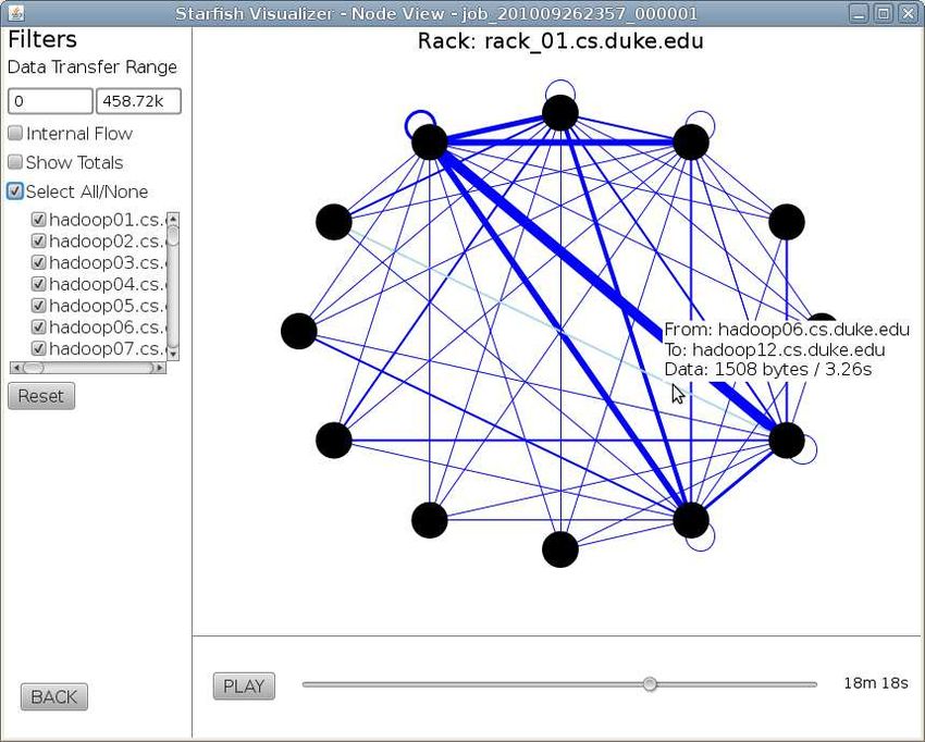
Figure 1: Starfish in the Hadoop ecosystem
   • Heavy use of programming languages: A sizable fraction                   1.1 Starfish: MADDER and Self-Tuning Hadoop
     of MapReduce programs will continue to be written in pro-                   Hadoop has the core mechanisms to be MADDER than exist-
     gramming languages like Java for performance reasons, or                 ing analytics systems. However, the use of most of these mecha-
     in languages like Python or R that a user is most comfortable            nisms has to be managed manually. Take elasticity as an example.
     with while prototyping new analysis tasks.                               Hadoop supports dynamic node addition as well as decommission-
                                                                              ing of failed or surplus nodes. However, these mechanisms do not
Traditional data warehouses are kept nonMAD by its administra-                magically make Hadoop elastic because of the lack of control mod-
tors because it is easier to meet performance requirements in tightly         ules to decide (a) when to add new nodes or to drop surplus nodes,
controlled environments; a luxury we cannot afford any more [6].              and (b) when and how to rebalance the data layout in this process.
To further complicate matters, three more features in addition to                Starfish is a MADDER and self-tuning system for analytics on
MAD are becoming important in analytics systems: Data-lifecycle-              big data. An important design decision we made is to build Starfish
awareness, Elasticity, and Robustness. A system with all six fea-             on the Hadoop stack as shown in Figure 1. (That is not to say that
tures would be MADDER than current analytics systems.                         Starfish uses Hadoop as is.) Hadoop, as observed earlier, has useful
Data-lifecycle-awareness: A data-lifecycle-aware system goes be-              primitives to help meet the new requirements of big data analytics.
yond query execution to optimize the movement, storage, and pro-              In addition, Hadoop’s adoption by academic, government, and in-
cessing of big data during its entire lifecycle. The intelligence em-         dustrial organizations is growing at a fast pace.
bedded in many Web sites like LinkedIn and Yahoo!—e.g., recom-                   A number of ongoing projects aim to improve Hadoop’s peak
mendation of new friends or news articles of potential interest, se-          performance, especially to match the query performance of parallel
lection and placement of advertisements—is driven by computation-             database systems [1, 7, 10]. Starfish has a different goal. The peak
intensive analytics. A number of companies today use Hadoop for               performance a manually-tuned system can achieve is not our pri-
such analytics [12]. The input data for the analytics comes from              mary concern, especially if this performance is for one of the many
dozens of different sources on user-facing systems like key-value             phases in the data lifecycle. Regular users may rarely see perfor-
stores, databases, and logging services (Figure 1). The data has to           mance close to this peak. Starfish’s goal is to enable Hadoop users
be moved for processing to the analytics system. After processing,            and applications to get good performance automatically through-
the results are loaded back in near real-time to user-facing systems.         out the data lifecycle in analytics; without any need on their part to
Terabytes of data may go through this cycle per day [12]. In such             understand and manipulate the many tuning knobs available.
settings, data-lifecycle-awareness is needed to: (i) eliminate indis-            Section 2 gives an overview of Starfish while Sections 3–5 de-
criminate data copying that causes bloated storage needs (as high as          scribe its components. The primary focus of this paper is on using
20x if multiple departments in the company make their own copy                experimental results to illustrate the challenges in each component
of the data for analysis [17]); and (ii) reduce resource overheads            and to motivate Starfish’s solution approach.
and realize performance gains due to reuse of intermediate data or
learned metadata in workflows that are part of the cycle [8].                 2. OVERVIEW OF STARFISH
Elasticity: An elastic system adjusts its resource usage and oper-               The workload that a Hadoop deployment runs can be considered
ational costs to the workload and user requirements. Services like            at different levels. At the lowest level, Hadoop runs MapReduce
Amazon Elastic MapReduce have created a market for pay-as-you-                jobs. A job can be generated directly from a program written in
go analytics hosted on the cloud. Elastic MapReduce provisions                a programming language like Java or Python, or generated from a
and releases Hadoop clusters on demand, sparing users the hassle              query in a higher-level language like HiveQL or Pig Latin [15], or
of cluster setup and maintenance.                                             submitted as part of a MapReduce job workflow by systems like
Robustness: A robust system continues to provide service, possi-              Azkaban, Cascading, Elastic MapReduce, and Oozie. The execu-
bly with graceful degradation, in the face of undesired events like           tion plan generated for a HiveQL or Pig Latin query is usually a
hardware failures, software bugs [12], and data corruption.                   workflow. Workflows may be ad-hoc, time-driven (e.g., run every

                                                                        262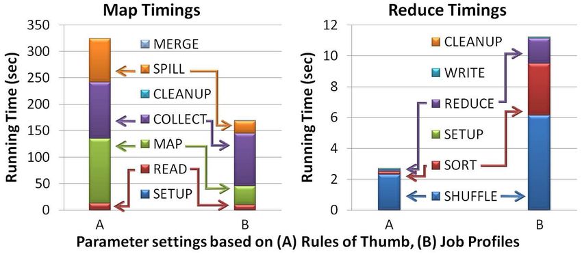
Figure 2: Example analytics workload to be run on Amazon Elastic MapReduce
gorized into job-level tuning, workflow-level tuning, and workload-
level tuning. These components interact to provide Starfish’s self-
tuning capabilities.
2.1 Job-level Tuning
The behavior of a MapReduce job in Hadoop is controlled by
the settings of more than 190 configuration parameters. If the user
does not specify parameter settings during job submission, then de-
fault values—shipped with the system or specified by the system
administrator—are used. Good settings for these parameters de-
pend on job, data, and cluster characteristics. While only a frac-
tion of the parameters can have significant performance impact,
browsing through the Hadoop, Hive, and Pig mailing lists reveals
that users often run into performance problems caused by lack of
knowledge of these parameters.
Figure 3: Components in the Starfish architecture Consider a user who wants to perform a join of data in the files
users.txt and geoinfo.txt, and writes the Pig Latin script:
hour), or data-driven. Yahoo! uses data-driven workflows to gener-
ate a reconfigured preference model and an updated home-page for Users = Load ‘users.txt’ as (username: chararray,
any user within seven minutes of a home-page click by the user. age: int, ipaddr: chararray)
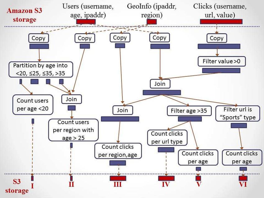
Figure 2 is a visual representation of an example workload that a GeoInfo = Load ‘geoinfo.txt’ as (ipaddr: chararray,
region: chararray)
data analyst may want to run on demand or periodically using Ama- Result = Join Users by ipaddr, GeoInfo by ipaddr
zon Elastic MapReduce. The input data processed by this workload
resides as files on Amazon S3. The final results produced by the The schema as well as properties of the data in the files could have
workload are also output to S3. The input data consists of files that been unknown so far. The system now has to quickly choose the
are collected by a personalized Web-site like my.yahoo.com. join execution technique—given the limited information available
The example workload in Figure 2 consists of workflows that so far, and from among 10+ ways to execute joins in Starfish—as
load the files from S3 as three datasets: Users, GeoInfo, and Clicks. well as the corresponding settings of job configuration parameters.
The workflows process these datasets in order to generate six dif- Starfish’s Just-in-Time Optimizer addresses unique optimization
ferent results I-VI of interest to the analyst. For example, Result problems like those above to automatically select efficient execu-
I in Figure 2 is a count of all users with age less than 20. For all tion techniques for MapReduce jobs. “Just-in-time” captures the
users with age greater than 25, Result II counts the number of users online nature of decisions forced on the optimizer by Hadoop’s
per geographic region. For each workflow, one or more MapRe- MADDER features. The optimizer takes the help of the Profiler
duce jobs are generated in order to run the workflow on Amazon and the Sampler. The Profiler uses a technique called dynamic in-
Elastic MapReduce or on a local Hadoop cluster. For example, no- strumentation to learn performance models, called job profiles, for
tice from Figure 2 that a join of the Users and GeoInfo datasets is unmodified MapReduce programs written in languages like Java
needed in order to generate Result II. This logical join operation and Python. The Sampler collects statistics efficiently about the
can be processed using a single MapReduce job. input, intermediate, and output key-value spaces of a MapReduce
The tuning challenges present at each level of workload process- job. A unique feature of the Sampler is that it can sample the exe-
ing led us to the Starfish architecture shown in Figure 3. Broadly, cution of a MapReduce job in order to enable the Profiler to collect
the functionality of the components in this architecture can be cate- approximate job profiles at a fraction of the full job execution cost.
263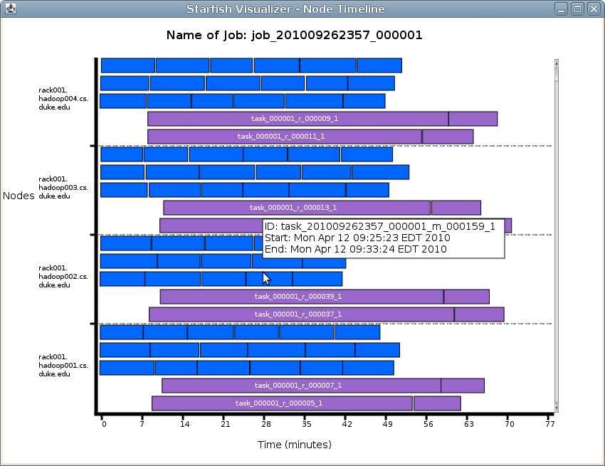
2.2 Workflow-level Tuning                                                         Hadoop provisioning deals with choices like the number of nodes,
   Workflow execution brings out some critical and unanticipated               node configuration, and network configuration to meet given work-
interactions between the MapReduce task scheduler and the un-                  load requirements. Historically, such choices arose infrequently
derlying distributed filesystem. Significant performance gains are             and were dealt with by system administrators. Today, users who
realized in parallel task scheduling by moving the computation to              provision Hadoop clusters on demand using services like Ama-
the data. By implication, the data layout across nodes in the clus-            zon Elastic MapReduce and Hadoop On Demand are required to
ter constrains how tasks can be scheduled in a “data-local” fash-              make provisioning decisions on their own. Starfish’s Elastisizer
ion. Distributed filesystems have their own policies on how data               automates such decisions. The intelligence in the Elastisizer comes
written to them is laid out. HDFS, for example, always writes the              from a search strategy in combination with the What-if Engine that
first replica of any block on the same node where the writer (in               uses a mix of simulation and model-based estimation to answer
this case, a map or reduce task) runs. This interaction between                what-if questions regarding workload performance on a specified
data-local scheduling and the distributed filesystem’s block place-            cluster configuration. In the longer term, we aim to automate provi-
ment policies can lead to an unbalanced data layout across nodes in            sioning decisions at the level of multiple virtual and elastic Hadoop
the cluster during workflow execution; causing severe performance              clusters hosted on a single shared Hadoop cluster to enable Hadoop
degradation as we will show in Section 4.                                      Analytics as a Service.
   Efficient scheduling of a Hadoop workflow is further compli-
cated by concerns like (a) avoiding cascading reexecution under                2.4 Lastword: Starfish’s Language for Work-
node failure or data corruption [11], (b) ensuring power propor-                   loads and Data
tional computing, and (c) adapting to imbalance in load or cost of                As described in Section 1.1 and illustrated in Figure 1, Starfish
energy across geographic regions and time at the datacenter level              is built on the Hadoop stack. Starfish interposes itself between
[16]. Starfish’s Workflow-aware Scheduler addresses such concerns              Hadoop and its clients like Pig, Hive, Oozie, and command-line
in conjunction with the What-if Engine and the Data Manager.                   interfaces to submit MapReduce jobs. These Hadoop clients will
This scheduler communicates with, but operates outside, Hadoop’s               now submit workloads—which can vary from a single MapReduce
internal task scheduler.                                                       job, to a workflow of MapReduce jobs, and to a collection of mul-
                                                                               tiple workflows—expressed in Lastword1 to Starfish. Lastword is
2.3 Workload-level Tuning                                                      Starfish’s language to accept as well as to reason about analytics
   Enterprises struggle with higher-level optimization and provi-              workloads.
sioning questions for Hadoop workloads. Given a workload con-                     Unlike languages like HiveQL, Pig Latin, or Java, Lastword is
sisting of a collection of workflows (like Figure 2), Starfish’s Work-         not a language that humans will have to interface with directly.
load Optimizer generates an equivalent, but optimized, collection              Higher-level languages like HiveQL and Pig Latin were developed
of workflows that are handed off to the Workflow-aware Scheduler               to support a diverse user community—ranging from marketing an-
for execution. Three important categories of optimization opportu-             alysts and sales managers to scientists, statisticians, and systems
nities exist at the workload level:                                            researchers—depending on their unique analytical needs and pref-
  A. Data-flow sharing, where a single MapReduce job performs                  erences. Starfish provides language translators to automatically
     computations for multiple and potentially different logical               convert workloads specified in these higher-level languages to Last-
     nodes belonging to the same or different workflows.                       word. A common language like Lastword allows Starfish to exploit
                                                                               optimization opportunities among the different workloads that run
  B. Materialization, where intermediate data in a workflow is                 on the same Hadoop cluster.
     stored for later reuse in the same or different workflows.                   A Starfish client submits a workload as a collection of work-
     Effective use of materialization has to consider the cost of              flows expressed in Lastword. Three types of workflows can be rep-
     materialization (both in terms of I/O overhead and storage                resented in Lastword: (a) physical workflows, which are directed
     consumption [8]) and its potential to avoid cascading reexe-              graphs2 where each node is a MapReduce job representation; (b)
     cution of tasks under node failure or data corruption [11].               logical workflows, which are directed graphs where each node is a
                                                                               logical specification such as a select-project-join-aggregate (SPJA)
  C. Reorganization, where new data layouts (e.g., with partition-
                                                                               or a user-defined function for performing operations like partition-
     ing) and storage engines (e.g., key-value stores like HBase
                                                                               ing, filtering, aggregation, and transformations; and (c) hybrid work-
     and databases like column-stores [1]) are chosen automat-
                                                                               flows, where a node can be of either type.
     ically and transparently to store intermediate data so that
                                                                                  An important feature of Lastword is its support for expressing
     downstream jobs in the same or different workflows can be
                                                                               metadata along with the tasks for execution. Workflows specified
     executed very efficiently.
                                                                               in Lastword can be annotated with metadata at the workflow level
While categories A, B, and C are well understood in isolation, ap-             or at the node level. Such metadata is either extracted from in-
plying them in an integrated manner to optimize MapReduce work-                puts provided by users or applications, or learned automatically by
loads poses new challenges. First, the data output from map tasks              Starfish. Examples of metadata include scheduling directives (e.g.,
and input to reduce tasks in a job is always materialized in Hadoop            whether the workflow is ad-hoc, time-driven, or data-driven), data
in order to enable robustness to failures. This data—which today is            properties (e.g., full or partial schema, samples, and histograms),
simply deleted after the job completes—is key-value-based, sorted              data layouts (e.g., partitioning, ordering, and collocation), and run-
on the key, and partitioned using externally-specified partitioning            time monitoring information (e.g., execution profiles of map and
functions. This unique form of intermediate data is available almost           reduce tasks in a job).
for free, bringing new dimensions to questions on materialization                 The Lastword language gives Starfish another unique advantage.
and reorganization. Second, choices for A, B, and C potentially in-            Note that Starfish is primarily a system for running analytics work-
teract among each other and with scheduling, data layout policies,
                                                                               1
as well as job configuration parameter settings. The optimizer has                 Language for Starfish Workloads and Data.
                                                                               2
to be aware of such interactions.                                                  Cycles may be needed to support loops or iterative computations.

                                                                         264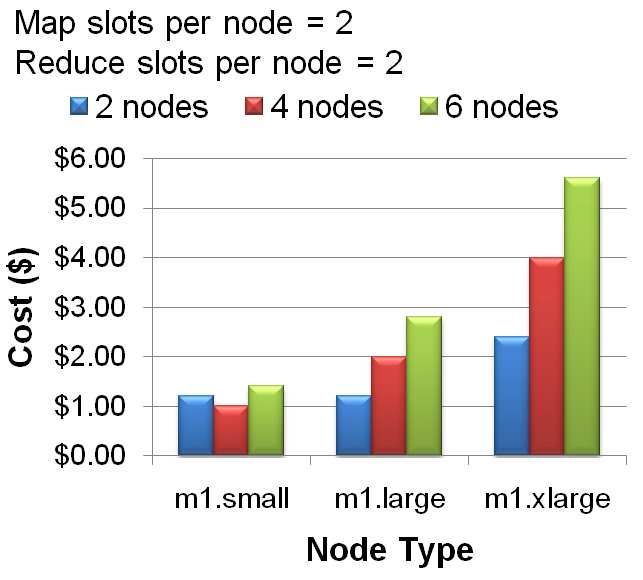
WordCount                 TeraSort                years to understand, debug, and optimize complex systems [4]. The
                          Rules of   Based on     Rules of    Based on
                          Thumb     Job Profile   Thumb      Job Profile         dynamic nature means that there is zero overhead when instrumen-
 io.sort.spill.percent     0.80        0.80        0.80         0.80             tation is turned off; an appealing property in production deploy-
 io.sort.record.percent    0.50        0.05        0.15         0.15             ments. The current implementation of the Profiler uses BTrace [2],
 io.sort.mb                 200         50          200          200             a safe and dynamic tracing tool for the Java platform.
 io.sort.factor             10          10           10          100                When Hadoop runs a MapReduce job, the Starfish Profiler dy-
 mapred.reduce.tasks        27          2            27          400             namically instruments selected Java classes in Hadoop to construct
 Running Time (sec)         785        407          891          606             a job profile. A profile is a concise representation of the job exe-
                                                                                 cution that captures information both at the task and subtask lev-
Table 1: Parameter settings from rules of thumb and recom-                       els. The execution of a MapReduce job is broken down into the
mendations from job profiles for WordCount and TeraSort                          Map Phase and the Reduce Phase. Subsequently, the Map Phase is
loads on big data. At the same time, we want Starfish to be usable in            divided into the Reading, Map Processing, Spilling, and Merging
environments where workloads are run directly on Hadoop without                  subphases. The Reduce Phase is divided into the Shuffling, Sorting,
going through Starfish. Lastword enables Starfish to be used as a                Reduce Processing, and Writing subphases. Each subphase repre-
recommendation engine in these environments. The full or partial                 sents an important part of the job’s overall execution in Hadoop.
Hadoop workload from such an environment can be expressed in                        The job profile exposes three views that capture various aspects
Lastword—we will provide tools to automate this step—and then                    of the job’s execution:
input to Starfish which is run in a special recommendation mode.
In this mode, Starfish uses its tuning features to recommend good                   1. Timings view: This view gives the breakdown of how wall-
configurations at the job, workflow, and workload levels; instead of                   clock time was spent in the various subphases. For exam-
running the workload with these configurations as Starfish would                       ple, a map task spends time reading input data, running the
do in its normal usage mode.                                                           user-defined map function, and sorting, spilling, and merging
                                                                                       map-output data.
3.    JUST-IN-TIME JOB OPTIMIZATION
   The response surfaces in Figure 4 show the impact of various                     2. Data-flow view: This view gives the amount of data pro-
job configuration parameter settings on the running time of two                        cessed in terms of bytes and number of records during the
MapReduce programs in Hadoop. We use WordCount and TeraSort                            various subphases.
which are simple, yet very representative, MapReduce programs.
The default experimental setup used in this paper is a single-rack                  3. Resource-level view: This view captures the usage trends of
Hadoop cluster running on 16 Amazon EC2 nodes of the c1.medium                         CPU, memory, I/O, and network resources during the vari-
type. Each node runs at most 3 map tasks and 2 reduce tasks con-                       ous subphases of the job’s execution. Usage of CPU, I/O,
currently. WordCount processes 30GB of data generated using the                        and network resources are captured respectively in terms of
RandomTextWriter program in Hadoop. TeraSort processes 50GB                            the time spent using these resources per byte and per record
of data generated using Hadoop’s TeraGen program.                                      processed. Memory usage is captured in terms of the mem-
                                                                                       ory used by tasks as they run in Hadoop.
Rules of Thumb for Parameter Tuning: The job configuration
parameters varied in Figure 4 are io.sort.mb, io.sort.record.percent,            We will illustrate the benefits of job profiles and the insights gained
and mapred.reduce.tasks. All other parameters are kept constant.                 from them through a real example. Figure 5 shows the Timings
Table 1 shows the settings of various parameters for the two jobs                view from the profiles collected for the two configuration parame-
based on popular rules of thumb used today [5, 13]. For exam-                    ter settings for WordCount shown in Table 1. We will denote the
ple, the rules of thumb recommend setting mapred.reduce.tasks                    execution of WordCount using the “Rules of Thumb” settings from
(the number of reduce tasks in the job) to roughly 0.9 times the                 Table 1 as Job A; and the execution of WordCount using the “Based
total number of reduce slots in the cluster. The rationale is to en-             on Job Profile” settings as Job B. Note that the same WordCount
sure that all reduce tasks run in one wave while leaving some slots              MapReduce program processing the same input dataset is being run
free for reexecuting failed or slow tasks. A more complex rule                   in either case. The WordCount program uses a Combiner to per-
                                                   16
of thumb sets io.sort.record.percent to 16+avg record    size
                                                              based on           form reduce-style aggregation on the map task side for each spill
the average size of map output records. The rationale here involves              of the map task’s output. Table 1 shows that Job B runs 2x faster
source-code details of Hadoop.                                                   than Job A.
   Figure 4 shows that the rule-of-thumb settings gave poor perfor-                 Our first observation from Figure 5 is that the map tasks in Job B
mance. In fact, the rule-of-thumb settings for WordCount gave one                completed on average much faster compared to the map tasks in Job
of its worst execution times: io.sort.mb and io.sort.record.percent              A; yet the reverse happened to the reduce tasks. Further exploration
were set too high. The interaction between these two parameters                  of the Data-flow and Resource views showed that the Combiner
was very different and more complex for TeraSort as shown in Fig-                in Job A was processing an extremely large number of records,
ure 4(b). A higher setting for io.sort.mb leads to better performance            causing high CPU contention. Hence, all the CPU-intensive op-
for certain settings of the io.sort.record.percent parameter, but hurts          erations in Job A’s map tasks (executing the user-provided map
performance for other settings. The complexity of the surfaces and               function, serializing and sorting the map output) were negatively
the failure of rules of thumb highlight the challenges a user faces              affected. Compared to Job A, the lower settings for io.sort.mb
if asked to tune the parameters herself. Starfish’s job-level tuning             and io.sort.record.percent in Job B led to more, but individually
components—Profiler, Sampler, What-if Engine, and Just-in-Time                   smaller, map-side spills. Because the Combiner is invoked on these
Optimizer—help automate this process.                                            individually smaller map-side spills in Job B, the Combiner caused
Profiling Using Dynamic Instrumentation: The Profiler uses dy-                   far less CPU contention in Job B compared to Job A.
namic instrumentation to collect run-time monitoring information                    On the other hand, the Combiner drastically decreases the amount
from unmodified MapReduce programs running on Hadoop. Dy-                        of intermediate data that is spilled to disk as well as transferred over
namic instrumentation has become hugely popular over the last few                the network (shuffled) from map to reduce tasks. Since the map

                                                                           265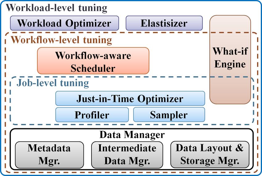
TeraSort in Hadoop
WordCount in Hadoop TeraSort in Hadoop
Settings
from
Rules of Settings
800 Thumb
1200 from
1150 Rules of
Running Time (sec)
750 Thumb
Running Time (sec)
1100
Running Time (sec)
700 1000
650 1050
600 1000 800
550 950
600
500 0
900 Settings
450 Settings 100
based on
based on 850 Job Profile
0.5
400 200
Job Profile 200 0.4
0.4 200
0.4 150 150 0.3
0.3 0.3
0.2 100 0.2 100 300 0.2
0.1 0.1
0 50 0.1
io.sort.mb 0 50 400
io.sort.record.percent io.sort.record.percent io.sort.mb mapred.reduce.tasks 0 io.sort.record.percent
Figure 4: Response surfaces of MapReduce programs in Hadoop: (a) WordCount, with io.sort.mb ∈ [50, 200] and
io.sort.record.percent ∈ [0.05, 0.5] (b) TeraSort, with io.sort.mb ∈ [50, 200] and io.sort.record.percent ∈ [0.05, 0.5] (c) TeraSort,
with io.sort.record.percent ∈ [0.05, 0.5] and mapred.reduce.tasks ∈ [27, 400]
4. The cluster setup and resource allocation that will be used to
run Job J. This information includes the number of nodes
and network topology of the cluster, the number of map and
reduce task slots per node, and the memory available for each
task execution.
The What-if Engine uses a set of performance models for predict-
ing (a) the flow of data going through each subphase in the job’s
execution, and (b) the time spent in each subphase. The What-if En-
gine then produces a virtual job profile by combining the predicted
Figure 5: Map and reduce time breakdown for two WordCount information in accordance with the cluster setup and resource allo-
jobs run with different settings of job configuration parameters cation that will be used to run the job. The virtual job profile con-
tasks in Job B processed smaller spills, the data reduction gains tains the predicted Timings and Data-flow views of the job when
from the Combiner were also smaller; leading to larger amounts run with the new parameter settings. The purpose of the virtual
of data being shuffled and processed by the reducers. However, profile is to provide the user with more insights on how the job will
the additional local I/O and network transfer costs in Job B were behave when using the new parameter settings, as well as to ex-
dwarfed by the reduction in CPU costs. pand the use of the What-if Engine towards answering hypothetical
Effectively, the more balanced usage of CPU, I/O, and network questions at the workflow and workload levels.
resources in the map tasks of Job B improved the overall perfor- Towards Cost-Based Optimization: Table 1 shows the parameter
mance of the map tasks significantly compared to Job A. Overall, settings for WordCount and TeraSort recommended by an initial
the benefit gained by the map tasks in Job B outweighed by far the implementation of the Just-in-Time Optimizer. The What-if En-
loss incurred by the reduce tasks; leading to the 2x better perfor- gine used the respective job profiles collected from running the jobs
mance of Job B compared to the performance of Job A. using the rules-of-thumb settings. WordCount runs almost twice
Predicting Job Performance in Hadoop: The job profile helps in as fast at the recommended setting. As we saw earlier, while the
understanding the job behavior as well as in diagnosing bottlenecks Combiner reduced the amount of intermediate data drastically, it
during job execution for the parameter settings used. More impor- was making the map execution heavily CPU-bound and slow. The
tantly, given a new setting S of the configuration parameters, the configuration setting recommended by the optimizer—with lower
What-if Engine can use the job profile and a set of models that we io.sort.mb and io.sort.record.percent—made the map tasks signif-
developed to estimate the new profile if the job were to be run using icantly faster. This speedup outweighed the lowered effectiveness
S. This what-if capability is utilized by the Just-in-Time Optimizer of the Combiner that caused more intermediate data to be shuffled
in order to recommend good parameter settings. and processed by the reduce tasks.
The What-if Engine is given four inputs when asked to predict These experiments illustrate the usefulness of the Just-in-Time
the performance of a MapReduce job J: Optimizer. One of the main challenges that we are addressing
is in developing an efficient strategy to search through the high-
1. The job profile generated for J by the Profiler. The profile dimensional space of parameter settings. A related challenge is in
may be available from a previous execution of J. Otherwise, generating job profiles with minimal overhead. Figure 6 shows the
the Profiler can work in conjunction with Starfish’s Sampler tradeoff between the profiling overhead (in terms of job slowdown)
to generate an approximate job profile efficiently. Figure 6 and the average relative error in the job profile views when profil-
considers approximate job profiles later in this section. ing is limited to a fraction of the tasks in WordCount. The results
are promising but show room for improvement.
2. The new setting S of the job configuration parameters using
which Job J will be run. 4. WORKFLOW-AWARE SCHEDULING
3. The size, layout, and compression information of the input Cause and Effect of Unbalanced Data Layouts: Section 2.2 men-
dataset on which Job J will be run. Note that this input tioned how interactions between the task scheduler and the policies
dataset can be different from the dataset used while gener- employed by the distributed filesystem can lead to unbalanced data
ating the job profile. layouts. Figure 7 shows how even the execution of a single large
266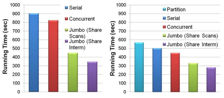
Figure 6: (a) Relative job slowdown, and (b) relative error in
the approximate views generated as the percentage of profiled                        Figure 8: Sort running time on the partitions
tasks in a job is varied

                                                                                             Figure 9: Partition creation time
                                                                               We ran the same partitioning job with a replication factor of two
                                                                            for the partitions. For our single-rack cluster, HDFS places the
                                                                            second replica of each block of the partitions on a randomly-chosen
               Figure 7: Unbalanced data layout                             node. The overall layout is still unbalanced, but the time to sort
job can cause an unbalanced layout in Hadoop. We ran a partition-           the partitions improved significantly because the second copy of
ing MapReduce job (similar to “Partition by age” shown in Figure            the data is spread out over the cluster (Figure 8). Interestingly, as
2) that partitions a 100GB TPC-H Lineitem table into four parti-            shown in Figure 9, the overhead of creating a second replica is very
tions relevant to downstream workflow nodes. The data properties            small on our cluster (which will change if the network becomes the
are such that one partition is much larger than the others. All the         bottleneck [11]).
partitions are replicated once as done by default for intermediate             Aside from ensuring that the data layout is balanced, other choices
workflow data in systems like Pig [11]. HDFS ends up placing all            are available such as collocating two or more datasets. Consider a
blocks for the large partition on the node (Datanode 14) where the          workflow consisting of three jobs. The first two jobs partition two
reduce task generating this partition runs.                                 separate datasets R and S (e.g., Users and GeoInfo from Figure
    A number of other causes can lead to unbalanced data layouts            2) using the same partitioning function into n partitions each. The
rapidly or over time: (a) skewed data, (b) scheduling of tasks in           third job, whose input consists of the outputs of the first two jobs,
a data-layout-unaware manner as done by the Hadoop schedulers               performs an equi-join of the respective partitions from R and S.
available today, and (c) addition or dropping of nodes without run-         HDFS does not provide the ability to collocate the joining parti-
ning costly data rebalancing operations. (HDFS does not automat-            tions from R and S; so a join job run in Hadoop will have to do
ically move existing data when new nodes are added.) Unbalanced             non-data-local reads for one of its inputs.
data layouts are a serious problem in big data analytics because               We implemented a new block placement policy in HDFS that
they are prominent causes of task failure (due to insufficient free         enables collocation of two or more datasets. (As an excellent ex-
disk space for intermediate map outputs or reduce inputs) and per-          ample of Hadoop’s extensibility, HDFS provides a pluggable inter-
formance degradation. We observed a more than 2x slowdown for               face that simplifies the task of implementing new block placement
a sort job running on the unbalanced layout in Figure 7 compared            policies [9].) Figure 10 shows how the new policy gives a 22%
to a balanced layout.                                                       improvement in the running time of a partition-wise join job by
    Unbalanced data layouts cause a dilemma for data-locality-aware         collocating the joining partitions.
schedulers (i.e., schedulers that aim to move computation to the               Experimental results like those above motivate the need for a
data). Exploiting data locality can have two undesirable conse-             Workflow-aware Scheduler that can run jobs in a workflow such
quences in this context: performance degradation due to reduced             that the overall performance of the workflow is optimized. Work-
parallelism, and worse, making the data layout further unbalanced           flow performance can be measured in terms of running time, re-
because new outputs will go to the over-utilized nodes. Figure 7            source utilization in the Hadoop cluster, and robustness to failures
also shows how running a map-only aggregation on the large par-             (e.g., minimizing the need for cascading reexecution of tasks due to
tition leads to the aggregation output being written to the over-           node failure or data corruption) and transient issues (e.g., reacting
utilized Datanode 14. The aggregation output was small. A larger            to the slowdown of a node due to temporary resource contention).
output could have made the imbalance much worse. On the other               As illustrated by Figures 7–10, good layouts of the initial (base),
hand, non-data-local scheduling (i.e., moving data to the computa-          intermediate (temporary), and final (results) data in a workflow are
tion) incurs the overhead of data movement. A useful new feature            vital to ensure good workflow performance.
in Hadoop will be to piggyback on such data movements to rebal-             Workflow-aware Scheduling: A Workflow-aware Scheduler can
ance the data layout.                                                       ensure that job-level optimization and scheduling policies are co-

                                                                      267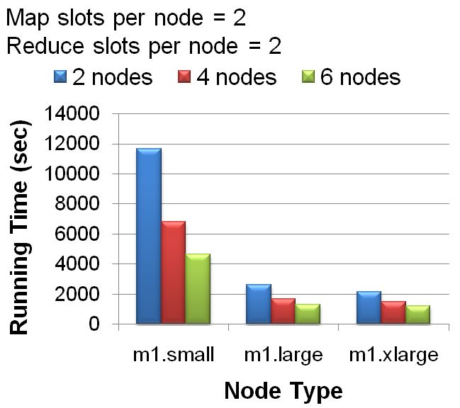
Figure 10: Respective execution times of a partition-wise join
job with noncollocated and collocated input partitions
ordinated tightly with the policies for data placement employed
by the underlying distributed filesystem. Rather than making de-
cisions that are locally optimal for individual MapReduce jobs,
Starfish’s Workflow-aware Scheduler makes decisions by consider-
ing producer-consumer relationships among jobs in the workflow.
   Figure 11 gives an example of producer-consumer relationships
among three Jobs P , C1, and C2 in a workflow. Analyzing these                Figure 11: Part of an example workflow showing producer-
relationships gives important information such as:                            consumer relationships among jobs
   • What parts of the data output by a job are used by down-                       block placement policy which works as follows: the first
     stream jobs in the workflow? Notice from Figure 11 that the                    replica of any block is stored on the same node where the
     three writer tasks of Job P generate files File1, File2, and                   block’s writer (a map or reduce task) runs. We have imple-
     File3 respectively. (In a MapReduce job, the writer tasks are                  mented a new Round Robin block placement policy in HDFS
     map tasks in a map-only job, and reduce tasks otherwise.)                      where the blocks written are stored on the nodes of the dis-
     Each file is stored as blocks in the distributed filesystem.                   tributed filesystem in a round robin fashion.
     (HDFS blocks are 64MB in size by default.) File1 forms the
     input to Job C1, while File1 and File2 form the input to Job                2. How many replicas to store—called the replication factor—
     C2. Since File3 is not used by any of the downstream jobs,                     for the blocks of a file? Replication helps improve perfor-
     a Workflow-aware Scheduler can configure Job P to avoid                        mance for heavily-accessed files. Replication also improves
     generating File3.                                                              robustness by reducing performance variability in case of
                                                                                    node failures.
   • What is the unit of data-level parallelism in each job that
     reads the data output by a job? Notice from Figure 11 that                  3. What size to use for blocks of a file? For a very big file, a
     the data-parallel reader tasks of Job C1 read and process one                  block size larger than the default of 64MB can improve per-
     data block each. However, the data-parallel reader tasks of                    formance significantly by reducing the number of map tasks
     Job C2 read one file each. (In a MapReduce job in a work-                      needed to process the file. The caveat is that the choice of the
     flow, the data-parallel map tasks of the job read the output                   block size interacts with the choice of job-level configuration
     of upstream jobs in the workflow.) While not shown in Fig-                     parameters like io.sort.mb (recall Section 3).
     ure 11, jobs like the join in Figure 10 consist of data-parallel
                                                                                 4. Should a job’s output files be compressed for storage? Like
     tasks that each read a group of files output by upstream jobs
                                                                                    the use of Combiners (recall Section 3), the use of compres-
     in the workflow. Information about the data-parallel access
                                                                                    sion enables the cost of local I/O and network transfers to be
     patterns of jobs is vital to guarantee good data layouts that,
                                                                                    traded for additional CPU cost. Compression is not always
     in turn, will guarantee an efficient mix of parallel and data-
                                                                                    beneficial. Furthermore, like the choice of the block size, the
     local computation. For File2 in Figure 11, all blocks in the
                                                                                    usefulness of compression depends on the choice of job-level
     file should be placed on the same node to ensure data-local
                                                                                    parameters.
     computation (i.e., to avoid having to move data to the compu-
     tation). The choice for File1, which is read by both Jobs C1             The Workflow-aware Scheduler performs a cost-based search for a
     and C2, is not so easy to make. The data-level parallelism is            good layout for the output data of each job in a given workflow.
     at the block-level in Job C1, but at the file-level in Job C2.           The technique we employ here asks a number of questions to the
     Thus, the optimal layout of File1 from Job C1’s perspective              What-if Engine; and uses the answers to infer the costs and benefits
     is to spread File1’s blocks across the nodes so that C1’s map            of various choices. The what-if questions asked for a workflow
     tasks can run in parallel across the cluster. However, the op-           consisting of the producer-consumer relationships among Jobs P ,
     timal layout of File1 from Job C2’s perspective is to place              C1, and C2 shown in Figure 11 include:
     all blocks on the same node.
                                                                                (a) What is the expected running time of Job P if the Round
Starfish’s Workflow-aware Scheduler works in conjunction with the                   Robin block placement policy is used for P ’s output files?
What-if Engine and the Just-in-Time Optimizer in order to pick the
job execution schedule as well as the data layouts for a workflow.              (b) What will the new data layout in the cluster be if the Round
The space of choices for data layout includes:                                      Robin block placement policy is used for P ’s output files?
   1. What block placement policy to use in the distributed filesys-            (c) What is the expected running time of Job C1 (C2) if its input
      tem for the output file of a job? HDFS uses the Local Write                   data layout is the one in the answer to Question (b)?

                                                                        268
Figure 13: Processing multiple SPA workflow nodes on the
Figure 12: Respective running times of (a) a partition job and
same input dataset
(b) a two-job workflow with the (default) Local Write and the
Round Robin block placement policies used in HDFS
uses the What-if Engine to do a cost-based estimation of whether
(d) What are the expected running times of Jobs C1 and C2 if the transformation will improve performance.
they are scheduled concurrently when Job P completes? Consider the workflows that produce the results IV, V, and VI
in Figure 2. These workflows have a join of Users and Clicks in
(e) Given the Local Write block placement policy and a repli- common. The results IV, V, and VI can each be represented as a
cation factor of 1 for Job P ’s output, what is the expected Select-Project-Aggregate (SPA) expression over the join. Starfish
increase in the running time of Job C1 if one node in the has an operator, called the Jumbo operator, that can process any
cluster were to fail during C1’s execution? number of logical SPA workflow nodes over the same table in a
single MapReduce job. (MRShare [14] and Pig [15] also support
These questions are answered by the What-if Engine based on a similar operators.) Without the Jumbo operator, each SPA node
simulation of the main aspects of workflow execution. This step in- will have to be processed as a separate job. The Jumbo operator en-
volves simulating MapReduce job execution, task scheduling, and ables sharing of all or some of the map-side scan and computation,
HDFS block placement policies. The job-level and cluster-level sorting and shuffling, as well as the reduce-side scan, computation,
information described in Section 3 is needed as input for the simu- and output generation. At the same time, the Jumbo operator can
lation of workflow execution. help the scheduler to better utilize the bounded number of map and
Figure 12 shows results from an experiment where the Workflow- reduce task slots in a Hadoop cluster.
aware Scheduler was asked to pick the data layout for a two-job Figure 13(a) shows an experimental result where three logical
workflow consisting of a partition job followed by a sort job. The SPA workflow nodes are processed on a 24GB dataset as: (a) Se-
choice for the data layout involved selecting which block place- rial, which runs three separate MapReduce jobs in sequence; (b)
ment policy to use between the (default) Local Write policy and the Concurrent, which runs three separate MapReduce jobs concur-
Round Robin policy. The remaining choices were kept constant: rently; (c) using the Jumbo operator to share the map-side scans
replication factor is 1, the block size is 128MB, and compression is in the SPA nodes; and (d) using the Jumbo operator to share the
not used. The choice of collocation was not considered since it is map-side scans as well as the intermediate data produced by the
not beneficial to collocate any group of datasets in this case. SPA nodes. Figure 13(a) shows that sharing the sorting and shuf-
The Workflow-aware Scheduler first asks what-if questions re- fling of intermediate data, in addition to sharing scans, provides
garding the partition job. The What-if Engine predicted correctly additional performance benefits.
that the Round Robin policy will perform better than the Local Now consider the workflows that produce results I, II, IV, and
Write policy for the output data of the partition job. In our cluster V in Figure 2. These four workflows have filter conditions on
setting on Amazon EC2, the local I/O within a node becomes the the age attribute in the Users dataset. Running a MapReduce job
bottleneck before the parallel writes of data blocks to other storage to partition Users based on ranges of age values will enable the
nodes over the network. Figure 12(a) shows the actual performance four workflows to prune out irrelevant partitions efficiently. Figure
of the partition job for the two block placement policies. 13(b) shows the results from applying partition pruning to the same
The next set of what-if questions have to do with the performance three SPA nodes from Figure 13(a). Generating the partitions has
of the sort job for different layouts of the output of the partition job. significant overhead—as seen in Figure 13(b)—but possibilities ex-
Here, using the Round Robin policy for the partition job’s output ist to hide or reduce this overhead by combining partitioning with a
emerges a clear winner. The reason is that the Round Robin policy previous job like data copying. Partition pruning improves the per-
spreads the blocks over the cluster so that maximum data-level par- formance of all MapReduce jobs in our experiment. At the same
allelism of sort processing can be achieved while performing data- time, partition pruning decreases the performance benefits provided
local computation. Overall, the Workflow-aware Scheduler picks by the Jumbo operator. These simple experiments illustrate the in-
the Round Robin block placement policy for the entire workflow. teractions among different optimization opportunities that exist for
As seen in Figure 12(b), this choice leads to the minimum total run- Hadoop workloads.
ning time of the two-job workflow. Use of the Round Robin policy Elastisizer: Users can now leverage pay-as-you-go resources on
gives around 30% reduction in total running time compared to the the cloud to meet their analytics needs. Amazon Elastic MapRe-
default Local Write policy. duce allows users to instantiate a Hadoop cluster on EC2 nodes,
5. OPTIMIZATION AND PROVISIONING and run workflows. The typical workflow on Elastic MapReduce
accesses data initially from S3, does in-cluster analytics, and writes
FOR HADOOP WORKLOADS final output back to S3 (Figure 2). The cluster can be released when
Workload Optimizer: Starfish’s Workload Optimizer represents the workflow completes, and the user pays for the resources used.
the workload as a directed graph and applies the optimizations listed While Elastic MapReduce frees users from setting up and main-
in Section 2.3 as graph-to-graph transformations. The optimizer taining Hadoop clusters, the burden of cluster provisioning is still
269Figure 14: Workload performance under various cluster and Hadoop configurations on Amazon Elastic MapReduce
Figure 15: Performance Vs. pay-as-you-go costs for a workload on Amazon Elastic MapReduce
on the user. Specifically, users have to specify the number and type tempted to use in the What-if Engine. However, Mumak needs a
of EC2 nodes (from among 10+ types) as well as whether to copy workload execution trace for a specific cluster size as input, and
data from S3 into the in-cluster HDFS. The space of provisioning cannot simulate workload execution for a different cluster size.
choices is further complicated by Amazon Spot Instances which
provide a market-based option for leasing EC2 nodes. In addition,
6. RELATED WORK AND SUMMARY
the user has to specify the Hadoop-level as well as job-level con- Hadoop is now a viable competitor to existing systems for big
figuration parameters for the provisioned cluster. data analytics. While Hadoop currently trails existing systems in
One of the goals of Starfish’s Elastisizer is to automatically deter- peak query performance, a number of research efforts are address-
mine the best cluster and Hadoop configurations to process a given ing this issue [1, 7, 10]. Starfish fills a different void by enabling
workload subject to user-specified goals (e.g., on completion time Hadoop users and applications to get good performance automat-
and monetary costs incurred). To illustrate this problem, Figure 14 ically throughout the data lifecycle in analytics; without any need
shows how the performance of a workload W consisting of a sin- on their part to understand and manipulate the many tuning knobs
gle workflow varies across different cluster configurations (number available. A system like Starfish is essential as Hadoop usage con-
and type of EC2 nodes) and corresponding Hadoop configurations tinues to grow beyond companies like Facebook and Yahoo! that
(number of concurrent map and reduce slots per node). have considerable expertise in Hadoop. New practitioners of big
The user could have multiple preferences and constraints for the data analytics like computational scientists and systems researchers
workload, which poses a multi-objective optimization problem. For lack the expertise to tune Hadoop to get good performance.
example, the goal may be to minimize the monetary cost incurred to Starfish’s tuning goals and solutions are related to projects like
run the workload, subject to a maximum tolerable workload com- Hive, Manimal, MRShare, Nectar, Pig, Quincy, and Scope [3, 8, 14,
pletion time. Figures 15(a) and 15(b) show the running time as well 15, 18]. The novelty in Starfish’s approach comes from how it fo-
as cost incurred on Elastic MapReduce for the workload W for dif- cuses simultaneously on different workload granularities—overall
ferent cluster configurations. Some observations from the figures: workload, workflows, and jobs (procedural and declarative)—as
• If the user wants to minimize costs subject to a completion time well as across various decision points—provisioning, optimization,
of 30 minutes, then the Elastisizer should recommend a cluster scheduling, and data layout. This approach enables Starfish to han-
of four m1.large EC2 nodes. dle the significant interactions arising among choices made at dif-
• If the user wants to minimize costs, then two m1.small nodes ferent levels.
are best. However, the Elastisizer can suggest that by paying
just 20% more, the completion time can be reduced by 2.6x. 7. REFERENCES
To estimate workload performance for various cluster configura- [1] A. Abouzeid, K. Bajda-Pawlikowski, D. J. Abadi, A. Rasin,
tions, the Elastisizer invokes the What-if Engine which, in turn, and A. Silberschatz. HadoopDB: An Architectural Hybrid of
uses a mix of simulation and model-based estimation. As dis- MapReduce and DBMS Technologies for Analytical
cussed in Section 4, the What-if Engine simulates the task schedul- Workloads. PVLDB, 2(1), 2009.
ing and block-placement policies over a hypothetical cluster, and [2] BTrace: A Dynamic Instrumentation Tool for Java.
uses performance models to predict the data flow and performance http://kenai.com/projects/btrace.
of the MapReduce jobs in the workload. The latest Hadoop release [3] M. J. Cafarella and C. Ré. Manimal: Relational Optimization
includes a Hadoop simulator, called Mumak, that we initially at- for Data-Intensive Programs. In WebDB, 2010.
270[4] B. M. Cantrill, M. W. Shapiro, and A. H. Leventhal. discover potential load balancing issues.
Dynamic Instrumentation of Production Systems. In Moreover, Timeline views can be used to compare different ex-
USENIX Annual Technical Conference, 2004. ecutions of the same job run at different times or with different
[5] Cloudera: 7 tips for Improving MapReduce Performance. parameter settings. Comparison of timelines will show whether
http://www.cloudera.com/blog/2009/12/ the job behavior changed over time as well as help understand the
7-tips-for-improving-mapreduce-performance. impact that changing parameter settings has on job execution. In
[6] J. Cohen, B. Dolan, M. Dunlap, J. M. Hellerstein, and addition, the Timeline views support a What-if mode using which
C. Welton. MAD Skills: New Analysis Practices for Big the user can visualize what the execution of a job will be when run
Data. PVLDB, 2(2), 2009. using different parameter settings. For example, the user can deter-
[7] J. Dittrich, J.-A. Quiané-Ruiz, A. Jindal, Y. Kargin, V. Setty, mine the impact of decreasing the value of io.sort.mb on map task
and J. Schad. Hadoop++: Making a Yellow Elephant Run execution. Under the hood, the Visualizer invokes the What-if En-
Like a Cheetah. PVLDB, 3(1), 2010. gine to generate a virtual job profile for the job in the hypothetical
[8] P. K. Gunda, L. Ravindranath, C. A. Thekkath, Y. Yu, and setting (recall Section 3).
L. Zhuang. Nectar: Automatic Management of Data and A.2 Data-flow Views
Computation in Datacenters. In OSDI, 2010.
The Data-flow views enable visualization of the flow of data
[9] Pluggable Block Placement Policies in HDFS.
among the nodes and racks of a Hadoop cluster, and between the
issues.apache.org/jira/browse/HDFS-385.
map and reduce tasks of a job. They form an excellent way of iden-
[10] D. Jiang, B. C. Ooi, L. Shi, and S. Wu. The Performance of tifying data skew issues and realizing the need for a better parti-
MapReduce: An In-depth Study. PVLDB, 3(1), 2010.
tioner in a MapReduce job. Figure 17 presents the data flow among
[11] S. Y. Ko, I. Hoque, B. Cho, and I. Gupta. Making Cloud the nodes during the execution of a MapReduce job. The thickness
Intermediate Data Fault-tolerant. In SoCC, 2010. of each line is proportional to the amount of data that was shuffled
[12] TeraByte-scale Data Cycle at LinkedIn. between the corresponding nodes. The user also has the ability to
http://tinyurl.com/lukod6. specify a set of filter conditions (see the left side of Figure 17) that
[13] Hadoop MapReduce Tutorial. allows her to zoom in on a subset of nodes or on the large data
http://hadoop.apache.org/common/docs/r0. transfers. An important feature of the Visualizer is the Video mode
20.2/mapred_tutorial.html. that allows users to play back a job execution from the past. Us-
[14] T. Nykiel, M. Potamias, C. Mishra, G. Kollios, and ing the Video mode (Figure 17), the user can inspect how data was
N. Koudas. MRShare: Sharing Across Multiple Queries in processed and transfered between the map and reduce tasks of the
MapReduce. PVLDB, 3(1), 2010. job, and among nodes and racks of the cluster, as time went by.
[15] C. Olston, B. Reed, A. Silberstein, and U. Srivastava.
Automatic Optimization of Parallel Dataflow Programs. In A.3 Profile Views
USENIX Annual Technical Conference, 2008. In Section 3, we saw how a job profile contains a lot of useful
[16] A. Qureshi, R. Weber, H. Balakrishnan, J. V. Guttag, and information like the breakdown of task execution timings, resource
B. V. Maggs. Cutting the Electric Bill for Internet-scale usage, and data flow per subphase. The Profile views help visualize
Systems. In SIGCOMM, 2009. the job profiles, namely, the information exposed by the Timings,
[17] Agile Enterprise Analytics. Keynote by Oliver Ratzesberger Data-flow, and Resource-level views in a profile; allowing an in-
at the Self-Managing Database Systems Workshop 2010. depth analysis of the task behavior during execution. For example,
[18] J. Zhou, P.-Å. Larson, and R. Chaiken. Incorporating Figure 5 shows parts of two Profile views that display the break-
Partitioning and Parallel Plans into the SCOPE Optimizer. In down of time spent on average in each map and reduce task for two
ICDE, 2010. WordCount job executions. Job A was run using the parameter set-
tings as specified by rules of thumb, whereas Job B was run using
APPENDIX the settings recommended by the Just-in-time Optimizer (Table 1
in Section 3). The main difference caused by the two settings was
A. STARFISH’S VISUALIZER more, but smaller, map-side spills for Job B compared to Job A.
When a MapReduce job executes in a Hadoop cluster, a lot of in- We can observe that the map tasks in Job B completed on av-
formation is generated including logs, counters, resource utilization erage much faster compared to the map tasks in Job A; yet the
metrics, and profiling data. This information is organized, stored, reverse happened to the reduce tasks. The Profile views allow us to
and managed by Starfish’s Metadata Manager in a catalog that can see exactly which subphases benefit the most from the parameter
be viewed using Starfish’s Visualizer. A user can employ the Vi- settings. It is obvious from Figure 5 that the time spent perform-
sualizer to get a deep understanding of a job’s behavior during ex- ing the map processing and the spilling in Job B was significantly
ecution, and to ultimately tune the job. Broadly, the functionality lower compared to Job A.
of the Visualizer can be categorized into Timeline views, Data-flow On the other hand, the Combiner drastically decreases the amount
views, and Profile views. of intermediate data spilled to disk (which can be observed in the
Data-flow views not shown here). Since the map tasks in Job B
A.1 Timeline Views processed smaller spills, the reduction gains from the Combiner
were also smaller; leading to larger amounts of data being shuffled
Timeline views are used to visualize the progress of a job exe-
and processed by the reducers. The Profile views show exactly how
cution at the task level. Figure 16 shows the execution timeline of
much more time was spent in Job B for shuffling and sorting the
map and reduce tasks that ran during a MapReduce job execution.
intermediate data, as well as performing the reduce computation.
The user can observe information like how many tasks were run-
Overall, the benefit gained by the map tasks in Job B outweighed
ning at any point in time on each node, when each task started and
by far the loss incurred by the reduce tasks, leading to a 2x better
ended, or how many map or reduce waves occurred. The user is
performance than Job A.
able to quickly spot any variance in the task execution times and
271You can also read