An Optimal Control Perspective on Weather and Climate Modification
←
→
Page content transcription
If your browser does not render page correctly, please read the page content below
mathematics

Article
An Optimal Control Perspective on Weather and
Climate Modification
Sergei Soldatenko *              and Rafael Yusupov

                                          St. Petersburg Federal Research Center of the Russian Academy of Sciences, No. 39, 14-th Line,
                                          St. Petersburg 199178, Russia; yusupov@iias.spb.su
                                          * Correspondence: soldatenko@iias.spb.su; Tel.: +7-931-354-0598

                                          Abstract: Intentionally altering natural atmospheric processes using various techniques and tech-
                                          nologies for changing weather patterns is one of the appropriate human responses to climate change
                                          and can be considered a rather drastic adaptation measure. A fundamental understanding of the
                                          human ability to modify weather conditions requires collaborative research in various scientific
                                          fields, including, but not limited to, atmospheric sciences and different branches of mathematics.
                                          This article being theoretical and methodological in nature, generalizes and, to some extent, sum-
                                          marizes our previous and current research in the field of climate and weather modification and
                                          control. By analyzing the deliberate change in weather and climate from an optimal control and
                                          dynamical systems perspective, we get the ability to consider the modification of natural atmospheric
                                          processes as a dynamic optimization problem with an emphasis on the optimal control problem.
                                          Within this conceptual and unified theoretical framework for developing and synthesizing an optimal
                                          control for natural weather phenomena, the atmospheric process in question represents a closed-loop
                                          dynamical system described by an appropriate mathematical model or, in other words, by a set of
                                          differential equations. In this context, the human control actions can be described by variations of
                                the model parameters selected on the basis of sensitivity analysis as control variables. Application
                                   of the proposed approach to the problem of weather and climate modification is illustrated using a
Citation: Soldatenko, S.; Yusupov, R.     low-order conceptual model of the Earth’s climate system. For the sake of convenient interpretation,
An Optimal Control Perspective on         we provide some weather and climate basics, as well as we give a brief glance at control theory and
Weather and Climate Modification.         sensitivity analysis of dynamical systems.
Mathematics 2021, 9, 305. https://
doi.org/10.3390/math9040305               Keywords: optimal control; dynamical systems; sensitivity analysis; weather modification; geoengi-
                                          neering
Academic Editors: Andrea Scapellato
and Temirkhan Aleroev
Received: 19 December 2020
Accepted: 1 February 2021
                                          1. Introduction
Published: 4 February 2021
                                               Weather modification and geoengineering represent the deliberate alteration of atmo-
Publisher’s Note: MDPI stays neutral
                                          spheric and climate conditions, locally or globally, by humans using the available assets
with regard to jurisdictional claims in
                                          and resources based on the existing theoretical understanding of weather and climate
published maps and institutional affil-   processes (see [1–6] and references herein). Over the years, people have sought to modify
iations.                                  the environment, including the atmosphere, in an attempt to adapt to its ever-changing
                                          conditions. However, the scientific-based stage of modification of the environment, first of
                                          all meteorological processes, only began in the middle of the 20th century when scientists
                                          at the General Electric Research Laboratories suggested using dry ice to disperse clouds [7].
Copyright: © 2021 by the authors.
                                          Since the early 1960s, dozens of projects have been implemented around the world aimed
Licensee MDPI, Basel, Switzerland.
                                          at modifying various atmospheric phenomena including different types of clouds, precipi-
This article is an open access article
                                          tation, lighting, hail, tornadoes, thunderstorms, hurricanes, and tropical cyclones. In the
distributed under the terms and           current century, the study and assessment of the human ability to modify environmental
conditions of the Creative Commons        conditions has taken on a new sound in connection with climate change, which is caused
Attribution (CC BY) license (https://     by anthropogenic activities posing a serious threat to all of humanity [8]. To mitigate the
creativecommons.org/licenses/by/          impact of climate change on nature and society, scientists have proposed the use of tools
4.0/).                                    and methods of so-called geoengineering (e.g., [9–13]).

Mathematics 2021, 9, 305. https://doi.org/10.3390/math9040305                                           https://www.mdpi.com/journal/mathematics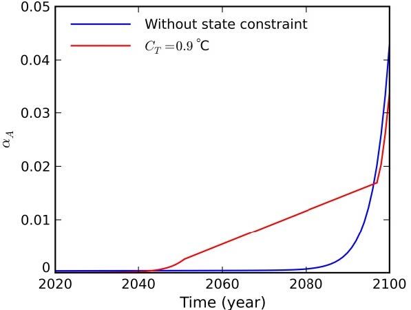
Mathematics 2021, 9, 305                                                                                            2 of 15

                                 However, we should make a difference between weather modification and geoengi-
                           neering. Weather characterizes the current atmospheric conditions in a certain area or point
                           at a particular time, or, in other words, the state of the atmosphere at some period of time is
                           described by such atmospheric variables as temperature, pressure, humidity, wind speed,
                           and direction, etc. Meanwhile, climate is the ensemble of states traversed by the Earth’s
                           climate system over a sufficiently long temporal interval (~30 years). In this regard, the
                           atmosphere, one of the five major components of the Earth’s climate system, is the most dy-
                           namic, unstable, and fastest-responding element of the climate system. The goal of weather
                           modification is to change weather conditions over some limited geographical area or some
                           geographical point. In other words, weather modification technologies are used to affect
                           processes only in the atmosphere, which, as was stated above, is the most variable element
                           of the climate system. In turn, geoengineering, being a planetary-scale process, is aimed
                           at neutralizing anthropogenic radiative forcing and thereby reducing or even preventing
                           human-caused warming of the Earth. Let us note that anthropogenic radiative forcing is
                           produced mainly by greenhouse gases (carbon dioxide CO2 , methane CH4 , nitrous oxide
                           N2 O, and fluorinated gases) entering the atmosphere via burning fossil fuels and industrial
                           and agricultural activities. However, both weather modification and geoengineering have
                           one thing in common: these two procedures are goal-oriented processes implemented by
                           means of external human-produced effects (interventions) to achieve specific objectives
                           under various constraints. Thus, deliberate modification of weather and climate is, in
                           substance, a dynamic optimization problem.
                                 By viewing the atmosphere and/or the climate as a controllable dynamical system, we
                           can approach weather modification and geoengineering from the perspective of optimal
                           control theory. Within this conceptual and unified theoretical framework, the purpose of
                           weather modification or geoengineering is formulated in terms of an extremal problem,
                           which involves finding control functions and the corresponding climate (atmospheric)
                           system trajectory that minimize or maximize a given objective function (also referred to
                           as performance measure or index) subject to various constraints. In this instance, the
                           atmospheric (climate) process in question is considered a closed-loop dynamical system,
                           the evolution of which is described by the appropriate mathematical model, commonly
                           represented by a set of differential equations. In this context, the human control actions
                           can be described by variations in the model parameters selected on the basis of sensitivity
                           analysis as control variables. This multi-disciplinary approach for planning and imple-
                           mentation of weather modification and geoengineering projects is known as geophysical
                           cybernetics, the theoretical foundations of which were laid by the authors of this paper in
                           the 1980s and ‘90s [14].
                                 This article is theoretical and methodological in nature aiming at generalizing and,
                           to some extent, summarizing our previous and current research related to weather and
                           climate modification and control. In the present paper, we first consider the deliberate
                           change in weather and climate from an optimal control and dynamical systems perspective
                           and, second, illustrate the application of this approach using a low-order conceptual model
                           of the Earth’s climate system. For the sake of convenient interpretation, we provide some
                           weather and climate basics, as well as giving a brief glance at control theory and sensitivity
                           analysis of dynamical systems relevant to weather and climate control.

                           2. Approach and Methods
                           2.1. Atmosphere and Climate as Dynamical Systems
                                The Earth’s climate system (ECS) and its components, the atmosphere, hydrosphere,
                           land surface, cryosphere, and biosphere, as control objects have some unique features that
                           are previously discussed in detail in [4]. The ECS is an open large-scale object affected by
                           different external forcing mechanisms including the anthropogenic one, but at the same
                           time, the impact of ECS on the external environment is minor. Each of the ECS subsystems
                           has specific dynamical, physical, and chemical properties. For example, the atmosphere
                           is the most variable and unstable component of the ECS having turbulent nature and
Mathematics 2021, 9, 305 3 of 15
showing wave-like oscillations over a wide-range time-space spectrum. ECS simulation,
and moreover, its control, is an extremely difficult problem due to a number of objective
reasons. First, ECS is an enormously complex natural object with many feedbacks and
cycles that are difficult to describe mathematically. Second, the ECS and its elements are not
fully identified as control objects; the corresponding mathematical models are not “perfect”,
and the degree of their reliability and validity is not always sufficiently high. Nevertheless,
over the last few decades, models of varying levels of complexity, from conceptual to
realistic, have become very powerful tools used for numerical weather prediction and
climate simulations [15–17].
Typically, deterministic mathematical models are used to numerically forecast weather
and study climate trends, while random mathematical models are applied to analyze
the variability of the climate system driven by stochastic forcing. For the purposes of
weather and climate modification and control, deterministic models are the primary focus.
In general terms, atmospheric (climate) models are systems of non-linear differential
equations in partial derivatives that are the mathematical statements of basic physical,
chemical, and biological laws. Such models also include a variety of empirical and semi-
empirical relationships and equations that are based on observations and experiences rather
than theories, and contain a large number of parameters that are considerably diverse in
their physical meaning. The equations describing the atmospheric and climate dynamics
are very complicated and, therefore, in most cases can be solved only numerically. To find
an approximate solution, various numerical techniques are usually used, for example, the
Galerkin projection method or the finite difference approach. As a result, atmospheric and
climate models are of finite space and time resolutions. Because of the limited time–spatial
resolutions of atmospheric and climate models, some physical, chemical, and biological
processes cannot be adequately resolved by the model space–time grid, and therefore can
be only parameterized leading to the significant increase in the model parameters. Some
model parameters are not well defined, generating parametric uncertainty in atmospheric
and climate models affecting the output results. Assessment of parametric uncertainty
is a very important component of model building and its quality assurance. Sensitivity
analysis in dynamical systems is among the most helpful tool for estimating the influence
of model parameters and their variations on the results of numerical simulations. It is
necessary to emphasize that both natural external forcing and purposeful and unintentional
human-caused forcing on the atmospheric (climate) system are described in atmospheric
(climate) models by means of variations in certain parameters. In this context, sensitivity
analysis serves as a tool for selecting parameters to be used as control variables.
An abstract dynamical system is a pair ( X, St ), where X is the system’s phase space
and St : X → X is a family of smooth evolution functions parameterized by a real variable
t ∈ T, the time. The set γs = { x (t) : t ∈ T} is called system’s trajectory (orbit), where
x (t) is continuous function with values in X such that Sτ x (t) = x (t + τ ) for all t ∈ T
and τ ∈ T+ . In atmospheric and climate studies, semi-dynamical systems are of primary
interest, for which a family {St : t ≥ 0} of mappings forms a one-parameter continuous
semigroup satisfying the following conditions [18]:
S0 ≡ I, where I is the identity operator for each t ≥ 0;
St+τ = St ◦ Sτ = Sτ ◦ St for all t, τ ≥ 0;
Sτ x is continuous in both t and x ∈ X.
Let us now consider continuous time finite dimensional deterministic dynamical
system with state vector x ∈ Rn and vector field f : Rn → Rn , generated by the following
set of autonomous ordinary differential equations (ODEs):
dx
= f ( x ), x (0 ) = x 0 ∈ Rn , (1)
dt
We consider an autonomous dynamical system only for convenience’s sake, since
any non-autonomous system of n unknown variables ( x1 , . . . , xn ) of t can formally be seen
as an autonomous system in n + 1 unknown variables (t, x1 , . . . , xn ). The state variablesMathematics 2021, 9, 305 4 of 15
(components of the state vector) representing a given atmospheric or climate system
include such physical quantities as the air and ocean temperatures, barometric pressure, air
density, humidity, wind velocity, and some others. It is very important that in atmospheric
and climate modelling, we are interested in the so-called “viable” state of a system in
question [19]. This means that the state vector belongs to the viable domain in state space
known as the viability constraint set, which can be formally defined by the condition
k x k < k x • k.
As mentioned above, in weather prediction and climate modeling, we deal with
discrete dynamical systems. Towards that end, using either a projection onto a finite set
of basic functions or a discretization of derivatives in time and space, the continuous
dynamical system (1) is transformed into discrete dynamical system xi+1 = f ( xi ), which
approximates the continuous system (1), and therefore can be solved numerically for given
initial conditions. Here xi denotes n-dimensional vector of state variables at discrete times
l ∈ Z+ .
It is important to note that deterministic models of the atmosphere and climate
possess some generic properties which must be borne in mind when modeling atmospheric
and climate processes, as well as when developing methods for controlling them. Some
of these properties are as follows. Firstly, deterministic models used in the numerical
weather prediction are very sensitive to initial conditions precluding exact forecasting
of weather and leading to chaotic oscillations in solutions of model equations. In other
words, over time, a phase space trajectory of the system bears a resemblance to random
process, although the system dynamics is determined by deterministic laws and described
by deterministic equations. This phenomenon known as deterministic chaos was first
uncovered by E. Lorenz [20]. Secondly, dynamical systems used in climate modeling are
dissipative, implying that the divergence of vector field ∇· f ( x (t)) is negative which leads
to contracting the system’s phase volume [21]. Thirdly, since climate dynamical systems are
dissipative, there exists a bounded absorbing set in the phase space that attracts trajectories
of climate system. This property assures the existence of a finite dimensional invariant
compact attracting set, called the attractor, toward which a dynamical system tends to
evolve over time [21].
Let us remark that small-scale physical processes cannot be always adequately repre-
sented on the space–time grid of existing deterministic atmospheric and climate models
and are perceived by these models as noise. To take into account the influence of these sub-
grid physical processes on the atmospheric and climate dynamics, one can use stochastic
dynamical systems generated by the following set of stochastic differential equations [22]:
dX = f ( X, t) + g( X, t)dW, (2)
where X ∈ Rn is the multidimensional stochastic process of interest possessing the initial
condition X |t=0 = X0 with probability one, W ∈ Rd is a vector of independent Wiener
processes, and g( X (t), t) is a matrix describing the dependence of the (sub-grid) noise on
the state vector. Stochastic models can be seen as useful tools for exploring the response of
the atmospheric (climate) system to random external forcing. In this case, the evolution of
the probability density function p( X, t) is determined using the Fokker–Planck equation
associated with Equation (2). However, the probabilistic formulation of the weather and
climate optimal control problem is beyond the scope of this article.
2.2. Sensitivity Analysis of Atmospheric and Climate Models
Atmospheric and climate models contain hundreds or even thousands of parame-
ters having different physical meanings. Some of them are empirical and semi-empirical,
while some others are adjustable and not well defined. Errors in the model parameters
generate parametric uncertainty. For convenience of further discussion, let us introduce the
k-dimensional parameter vector α ∈ Rk and then rewrite the set of autonomous ODEs (1) as
follows: dx/dt = f ( x, α), where x (0) = x0 ∈ Rn . The space–time spectrum of atmospheric
and climatic processes is very wide, therefore it is hardly possible to develop a “univer-Mathematics 2021, 9, 305 5 of 15
sal” model capable of covering a broad range of atmospheric and climatic fluctuations.
If the physical (dynamical) process of interest has a characteristic time τ, then all processes
whose scales are less than τ cannot be explicitly reproduced by the model and can only be
described parametrically. Based on physical considerations and using sensitivity analysis,
some of the model parameters can be selected as control variables [23]. Varying control
parameters, we can formally control the dynamics of atmospheric and climate processes.
In conventional sensitivity analysis [24], in its attempt to analyze the influence of
model parameters (forcing functions) on state variables, sensitivity functions (coefficients)
are usually used, defined as partial derivatives of the state vector components with respect
to the model parameters. For example, the sensitivity of the state variable xi (i = 1, . . . , n)
with respect to the parameter α j ( j = 1, . . . , k) is estimated using the following sensitivity
function: Sij = ∂xi (t, α)/∂α j α0 , where α0j is a base value of the parameter α j at which
j
the partial derivative is estimated. Assuming that δα j is an infinitesimal (infinitely small)
change in the parameter α j with respect to its unperturbed value α0j , then, approximating
the state vector around its base value x (α0j ) by the Taylor expansion, we get the following
expression for the corresponding change in the vector of state variables:
δx (δα0j ) = x (α0j + δα j ) − x (α0j ) = ∂x/∂α j α0j
· δα j + H.O.T. (3)
However, the absolute changes in the state vector caused by variations in different
parameters do not allow the parameters to be ranked in accordance with the degree of their
influence on the state vector, since the model parameters have different units. To compare
the relative role of model parameters in changing δx, and thereby to rank the parameters,
we can use relative sensitivity functions defined as
α j ∂xi
SijR = , (4)
xi ∂α j
α0j
Relative sensitivity functions play a very important role in the justification and selec-
tion of those parameters that can be considered as physically feasible control variables [23].
For example, considering atmospheric baroclinic instability as a controllable object, we
have identified two fundamental parameters that govern the development of baroclinic
instability in the atmosphere: the static stability parameter σ0 and the vertical wind shear
Λ0 induced by the meridional temperature gradient. Analyzing the relative sensitivity
functions, we found the critical value of the wavelength Lcr of the growing modes that
divides the spectrum of unstable waves into two parts. The growth rates of the amplitudes
of unstable waves, the length of which is shorter than Lcr , depend mainly on the static
stability parameter, while if L < Lcr , then the development of baroclinic instability is
predominantly affected by the vertical wind shear, that is, by the meridional temperature
gradient. For typical values of atmospheric parameters, we found that Ler = 3800 km.
Sensitivity functions can be found by solving the set of linear non-homogeneous
sensitivity equations obtained by differentiating the model equations with respect to
the parameters:
dSα ( x )
= Jx ( f )Sα ( x ) + Jα ( f ), (5)
dt
where Sα ( x ) = ∂xi /∂α j ∈ Rn×k is the sensitivity matrix, Jx ( f ) ∈ Rn×n and Jx ( f ) ∈ Rn×k
are the Jacobian matrices given by
Jx ( f ) = ∂ f i /∂x j , Jα ( f ) = ∂ f i /∂α j . (6)
These equations show how sensitivity functions evolve over time along the trajectory
of a dynamical system. To estimate the sensitivity of the state vector x with respect to the
parameter vector α, we need to solve a set of differential equations that includes the modelMathematics 2021, 9, 305 6 of 15
equations and the sensitivity equations with given initial conditions. However, due to the
large dimensionality of the parameter vector of modern atmospheric and climate models,
“direct” sensitivity analysis, considered above, is a computationally expensive process.
In addition, the derivation of sensitivity equations requires the sequential differentiation
of model equations with respect to the desired parameters, which is difficult to perform
for complex atmospheric and climate models. To overcome these difficulties, we can
introduce some response function R(x,α) and then examine its sensitivity with respect to
model parameters in a differential formulation using the adjoint model [25]. Formally, the
response function can be written as follows:
Zte
R( x, α) = Φ(t; x, α)dt, (7)
0
where Φ is a function that depends on the model state variables and parameters.
For example, this function can characterize the total energy norm of a dynamical sys-
tem Φ = xT Wx, where W is the matrix of weights defining the norm.
The gradient of the response function with respect to α at the base point α0 character-
izes the sensitivity of the model state variables to the model parameters. This “sensitivity”
gradient can be determined from a single numerical experiment by solving the following
equation [25]:
Zte
∂Φ
0 0
∇α R( x , α ) = − [ Jα ( f )] T α · x ∗ dt. (8)
∂α α0 α
0
where the superscript “T” means “transpose”, x0 is the trajectory of the dynamical system
corresponding to the parameter vector α0 , and the vector-valued function x ∗ is the solution
to the adjoint model:
∂x ∗ ∂Φ
+ [ Jx ( f )]T · x∗ = , x ∗ (te ) = 0. (9)
∂t α0 ∂x α0
The variation in the response function δR caused by the parameter variations is
calculated as follows: δR( x0 , α0 ) = h∇α R, δαi, where δR( x0 , α0 ) = h·, ·i is a scalar product.
It should be underlined that sensitivity analysis of chaotic dynamical systems used
in atmospheric and climate studies usually deserves special examination [26]. However,
this topic is beyond the scope of this paper, since it is not related to weather and climate
modification and control. A fairly complete and comprehensive survey of sensitivity
analysis for nonlinear dynamical systems exhibiting, under certain conditions, chaotic
behavior can be found in previously published papers (e.g., [27,28]).
2.3. Generic Formulation of the Optimal Control Problem
Intending to study weather and climate manipulations as an optimal control problem,
we will consider
h a continuous
i time deterministic dynamical system, evolving over a given
time interval t0 , t f , where the terminal time t f > 0 can either be free or fixed. Without
loss of generality, we will assume that t f is fixed. The state of a system at any instant of
h i
time t ∈ t0 , t f is characterized by the vector x ∈ Rn . We will suppose that the system
is controllable. In other words, the system can be moved from some initial state to any
other (desired) state in a finite time using certain external manipulations characterized
formally by the vector of control variables u ∈ Rm . By a system, we mean a set of ordinary
differential equations of the form:
dx
= f ( x, u), x (t0 ) = x0 ∈ Rn , (10)
dtMathematics 2021, 9, 305 7 of 15
h i
where f : t0 , t f × Rn × Rm → Rn is a given vector-valued function.
Note that the right-hand side of Equation (10) explicitly depends on the control
variables, while uncontrolled parameters are omitted for convenience. It is worth noting
that the control variables should be selected based on physical considerations, taking into
account the feasibility of technical implementation of deliberate modification of weather
and climate [4]. Thus, control variables are formally restricted to some control domain U
called as the admissible control set of u:
h i
u : t0 , t f 7→ u(t) ∈ U. (11)
Generally, various physical constraints, expressed mathematically in the form of
equalities and/or inequalities, can be imposed on state variables. Formally, this means that
the state vector must belong to a certain phase-space domain:
h i
x : t0 , t f 7→ x (t) ∈ X, , (12)
where X is a given subset of Rn .
Equations (10)–(12), considered together, restrict the set of admissible terminal values
of state variables, i.e., x (t f ) = x f ∈ X f , where X f is the set of reachable states.
In essence, an optimal control problem is aimed at finding the control law for a given
system that ensures the fulfillment of a control objective, which is usually the minimization
of some function (functional) J ( x, u), the objective functional (or performance index).
We should note that the formulation of a performance index is dependent on the problem
under study. To be more specific, can we consider the Bolza optimal control problem,
assuming that no constraints are imposed on the state and control variables, and the initial
and terminal times are fixed:
Z te
min L( x, u)dt + l ( x (te ), u(te )), (13)
u ∈U t 0 | {z }
| {z } f inal cos t
running cos t
subject to constraint
dx
= f ( x, u) (14)
dt
and the boundary conditions
x ( t0 ) = x0 , x ( t f ) = x f . (15)
An optimal control problem can be solved by Pontryagin’s maximum principle, dy-
namical programming, or classical approaches of the calculus of variations.
3. Illustrative Example
Holding the increase in global mean surface temperature “to well below 2 ◦ C above
pre-industrial levels and pursuing efforts to limit the temperature increase to 1.5 ◦ C above
pre-industrial levels” was designated in the 2015 Paris Agreement on Climate as a priority
area for combating global warming. This ambitious goal is expected to be achieved through
the transition to low-carbon development, which, on the one hand, is a vital necessity,
and on the other, a serious challenge. Nevertheless, many countries are already in the
transition to a low-carbon economy, developing national strategies to achieve the Paris
Agreement goals using, in particular, the Shared Socioeconomic Pathways scenarios of
projected social and economic worldwide changes up to 2100 [29]. However, the Earth’s
climate system possesses significant inertia (e.g., [30]): it takes several decades for the
climate system to reach a new equilibrium state in response to low (even zero) emissions
of greenhouse gases (GHG). Therefore, after significant reduction of atmospheric GHG
concentrations, surface temperature apparently will continue to rise. This phenomenonMathematics 2021, 9, 305 8 of 15
is known as “lag (time delays) between cause and effect”. Thus, geoengineering can be
considered as one of the technologically feasible options to stabilize the climate. In this
paper, we leave “behind brackets” of such important aspects of geoengineering as physical
side effects and environmental risks, ethical, legal and other social issues, recognizing the
importance of their consideration and assessment (e.g., [31]).
Geoengineering can be implemented via human intervention in the redistribution of
solar radiation flux due, for example, to the injection into the stratosphere of fine aerosol
particles, which have the properties to scatter solar radiation in the visible spectral range
and weakly absorb in the infrared range. For example, sulfate aerosols have such properties.
Controlled emissions of sulfur dioxide or hydrogen sulfide (precursor gases) into the
stratosphere ultimately lead to the formation of sulfate aerosol particles. The stratospheric
aerosols increase the Earth’s planetary albedo α0 , change the radiation balance, and, as
a consequence, decrease the Earth’s surface temperature. Sensitivity analysis shows that
an increase in α0 by 1% leads to a decrease in the solar radiation flux at the top of the
atmosphere by about 3.4 W/m2 , which is comparable with the radiation effect of doubling
the concentration of atmospheric CO2 . To assess the effectiveness of geoengineering
projects and their consequences for nature and society, numerical modeling is used for
given scenarios of anthropogenic GHG emissions and atmospheric concentrations, and
heuristically specified geoengineering scenarios. It is obvious that going through all
possible options of intentional geoengineering manipulations is an ineffective approach.
In contrast to that, we consider climate manipulation within the framework of the optimal
control theory. To illustrate this approach, we will apply the two-box low-parametric
climate model, taking into account the radiation effects of the sulfate aerosols artificially
injected into the stratosphere. The model equations are as follows [32]:
dt = − λT − γ ( T − TD ) + ∆R GHG + ∆R A
C dT
(16)
CD dTdt = γ ( T − TD )
D
where T and TD are temperature anomalies for the upper (the atmosphere and mixing
ocean layer) and lower (the deep ocean) boxes, C and CD are the effective heat capacities
for the upper and lower boxes, λ is a climate feedback parameter, γ is a coupling strength
parameter describing the rate of heat loss by the upper box, ∆RGHG is the radiative forcing
produced by GHG, and ∆R A is the radiative forcing generated by stratospheric aerosols.
The two-box model, in spite of its simplicity, is capable of simulating globally av-
eraged climate change caused by human-induced radiative forcing with a reasonable
accuracy (e.g., [33,34]). The following values of model parameters have been used in calcu-
2 K , C = 105.5 (W yr) / m2 K , λ = 1.13 W/ m2 K and
lations [31]: C = 7.34 ( W yr ) / m D
γ = 0.7 W/ m2 K . Radiative forcing ∆RGHG is approximated by a linear function
∆RGHG = ηt, where the parameter η is determined from the Representative Concen-
tration Pathway (RCP) data [35]. For the worst-case emission scenario (RCP8.5 [35]), the
annual radiative forcing rate is η = 7.14·10−2 W/ m2 yr . Radiative forcing produced by
aerosols is calculated by the formula: ∆R A = −α A Q0 , where α A is the albedo of the aerosol
layer (note that α AMathematics 2021, 9, 305 9 of 15
In practice, precursor gases are injected into the stratosphere, therefore the mass
of sulfate aerosols and their emission rate are expressed in sulfur units and denoted as
ES (TgS/year) and MS (TgS), respectively, taking into account that 1 Tg of sulfur is equiva-
lent to 4 Tg of aerosol particles. Then, Equation (17) can be rewritten as
dα A α
= χ −1 E A − A , (18)
dt τA
where χ = Q0 Se /4β A k a ≈ 2.39·102 TgS.
If the optimal albedo of aerosol layer is determined, then the optimal emission rate
ES∗ (t), which provides the formation of an aerosol layer of the optimal mass MS∗ (t), is
calculated using Equation (18).
The optimal control problem will be considered with regard to the finite time interval
t ∈ [t0 , te ] on which the dynamics of the control object are described by Equation (16) with
given boundary conditions:
T (t0 ) = 0, TD (t0 ) = 0, T (t f ) = T f . (19)
Thus, the left end of the phase trajectory is fixed, and the right end is fixed only for
the variable T, while the variable TD is free. These boundary conditions are chosen since
the surface temperature anomaly T is of primary interest. The optimal control problem is
formulated as follows: on the finite time interval [t0 , te ] find the control variable α∗A (t) belonging
to an admissible value domain, so that when the dynamic constraints (16) and boundary conditions
(19) imposed on the system are satisfied, the given functional characterizing the mass flow rate
of aerosols
1 te 2
Z
J= α (t)dt (20)
2 t0 A
has reached its minimum value.
The terminal condition T f represents a target change in the global mean surface tem-
perature at t = t f . As an example, we assume that T f = 2 ◦ C. In essence, the performance
index characterizes the consumption of aerosols for geoengineering manipulations since
the albedo of the aerosol layer α A is a linear function of M A . So, we aim at minimizing the
mass of aerosols required to achieve the target surface temperature change at final time
which is fixed. The amount of aerosols that can be annually delivered to the stratosphere
can be limited by the available technical capabilities. Therefore, we will formally assume
that the domain of admissible controls is an interval α A ∈ [0, U ], where U is the maximum
value of technically feasible albedo α A .
To solve the optimal control problem, we use the Pontryagin’s maximum principle
(PMP), which is the major tool in optimal control. The Hamiltonian function used to solve
the problem of optimal control for dynamical system (16) is given by:
1
H = − α2A + ψ1 (− aT + bTD + ct − qα A ) + ψ2 ( pT − pTD ), . (21)
2
where a = (λ + γ)/C; b = γ/C; c = η/C; q = (1 − α0 ) Q0 /C; p = γ/CS ; ψ1 and ψ2 are the
time-varying Lagrange multipliers that satisfy the adjoint equations:
dψ1 dψ2
= aT − pψ2 , = −bT + pψ2 . (22)
dt dt
The optimal control α∗A (t) ∈ [0, U ] at each fixed time t ∈ [t0 , t f ] must be such that
H (ψ1 , ψ2 , T, TD , α∗A ) ≥ H (ψ1 , ψ2 , T, TD , α A ). (23)Mathematics 2021, 9, 305 10 of 15
In other words, the optimal control results in a maximum value of H at any t ∈ [t0 , t f ]
α∗A = argmaxH (α A ). (24)
α A ∈[0,U ]
The corresponding stationarity conditions for Hamiltonian yields:
∂H
= −α A − qψ1 . (25)
dα A
To find the optimal control α∗A and the optimal surface temperature anomaly T ∗
generated by α∗A , we must solve the system of four ordinary Equations (16) and (21) in
four unknown variables ψ1 , ψ2 , T, and TD , with given initial and terminal conditions (18).
condition is specified for the variable TD , the following transversality
Since no terminal
condition ψ2 t f = 0 is used in calculations. We have derived the following analytical
expressions for the optimal albedo of aerosol layer α∗A and the corresponding optimal
surface temperature anomaly T ∗ :
α∗A (t) = −C1 q ν11 eλ1 t + e(λ1 −λ2 )t f ν21 eλ2 t , (26)
T ∗ (t) = C1 α1 eλ1 t − α2 eλ2 t + C3 e−λ1 t + C4 e−λ2 t + w1 t + w2 , (27)
where λ1 and λ2 are the eigenvalues of the coefficient matrix of the adjoint system (22),
ν11 and ν21 are the components of the corresponding eigenvectors, C1 , C2 , C3 , and C4 , are
arbitrary integration constants, while C2 = −C1 e(λ1 −λ2 )t f ,
q2 v11 (λ1 + p)
α1 = ,
λ21 + λ1 ( a + p) + ( ap − pb)
q2 v21 (λ2 + p)e(λ1 −λ2 )t f
α2 = ,
λ21 + λ1 ( a + p) + ( ap − pb)
pc
w1 = ,
ap − pb
c[( ap − pb) − p( a + p)]
w2 = .
( ap − pb)2
Considering geoengineering as a state-constrained optimal control problem
T ≤ CT ∀ t ∈ [ t 0 , t f ] , (28)
additional necessary conditions for optimality, the complementary slackness condition,
must be specified. The meaning of the path constraint condition (28) is that the global
mean surface temperature anomaly should not exceed the value of threshold parameter
CT , which is set a priori.
As an example, we consider the results of calculations for the RCP8.5 emission scenario
(as we mentioned earlier, this is the most conservative scenario in relation to the growth of
atmospheric GHG concentrations). The optimal control problem is examined on the finite
time interval 2020–2100. In other words, t0 = 2020 and t f = 2100. Since the temperature
anomalies are calculated relative to 2020, the initial conditions for variables T and TD are
as follows: T2020 = 0 and TD,2020 = 0, where the numerical subscript is referred to the year
2020. We assume that:
- By 2020, the surface temperature anomaly would exceed the pre-industrial level by
1.1 ◦ C, i.e., ∆T2020 = 1.1 ◦ C
- By 2100, the surface temperature anomaly would exceed the pre-industrial level by
1.5 ◦ C;Mathematics 2021, 9, 305 11 of 15
- For the 2020 to 2100 period of time, the increase in T should not exceed 2 ◦ C above the
pre-industrial level.
Then the allowable temperature growth by year 2100 relative to 2020 would be
◦
T2100 = ∆T2100 − ∆T2020 = 0.4 C. This value is taken as a terminal condition for
variable T at t = t f . The threshold parameter, which defines a path constraint, is
◦
CT = 2 − ∆T2020 = 0.9 C.
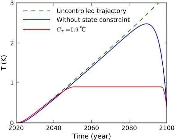
Calculations show that in the absence of deliberate interventions in the Earth’s climate
system, the growth of global average surface temperature over the 80-year (2020–2100)
interval is about 3.8 ◦ C which is significantly higher than the level established by the
Paris Agreement. Figure 1 presents two curves, one for the optimal albedo of the aerosol
cloud and the other for the corresponding surface temperature anomaly, as functions of
time calculated for the case (a) when no constraints are imposed on the control variable
thematics 2021, 9, x FOR PEER REVIEW and the surface temperature anomaly, and (b) with constraint imposed on the surface 12 o
temperature anomaly. As can be seen from Figure 1b, in the absence of limitations on the
surface temperature increase, beginning from 2060, some overshoot beyond the threshold
CT is observed. However, stratospheric aerosols, artificially injected into the stratosphere,
for the unconstrained
guarantee complianceoptimal controlterminal
with the specified problem, and 23.3
condition. Tgthat
Recall forthisthe problem
condition is aswith st
◦
constraint.
follows: T2100 = 0.4 C at t = 2100.
(a) (b)
Figure 1. Figure
Optimal albedoalbedo
1. Optimal of the aerosol
of the aerosollayer
layer (a) andthethe
(a) and corresponding
corresponding surfacesurface temperature
temperature anomalies
anomalies (b) (b) calculated
calculated with
with and without state
and without constraint.
state constraint.
The optimal control problem with state constraint requires the consideration of
4. Discussion
an additional necessary condition termed as a condition of complementary slackness:
◦
In
µ(tresponse
)[CT − T (t)]to≥ human-induced
0, where µ(t) ≥ 0 is climate change,
the Lagrange which
multiplier. For is
theone
case of
of Cthe
T =main
0.9 C threats
(see above), the optimal albedo and the corresponding surface temperature
natural and anthropogenic systems in the 21st century, the scientific meteorologi anomaly are
shown in Figure 1 in red color. As can be seen from this figure, by using state constraint, it
community has proposed several technologies known as geoengineering to deceler
is possible to prevent an undesirable growth of surface temperature within a given time
global warming
interval. and stabilize
The amount the
of aerosols climate.
required overHowever, all oftothese
an 80-year period technologies,
maintain geoengineer-includi
solar ing
radiation management
is 36.5 TgS (SRM) case
for the unconstraint considered
and 73.6 inTgSthis
for paper,
the casearewithstill theoretical
state constraint. in natu
sinceFor RCP6.0 scenario
“Playing with the (thisEarth’s
scenario climate
is described
is by the Intergovernmental
a dangerous game with Panelunclear
on Climate
rules” [3
Change as an intermediate scenario in which emissions’ peak is around 2080, then decline)
Nevertheless, scientists from different countries continue geoengineering research usi
we obtained that the total amount of aerosols is 17.0 Tg for the unconstrained optimal
mainly computer
control problem, simulations expecting
and 23.3 Tg for the problem that geoengineering
with state constraint. techniques could potentia
be helpful in the future to enhance ongoing efforts to mitigate global warming by
ducing4. Discussion
anthropogenic GHG emissions. Meanwhile, in the vast majority of studies
heuristic In response to
approach is human-induced
used to developing climate geoengineering
change, which is one of the main
strategies andthreats
scenarios (e
to natural and anthropogenic systems in the 21st century, the scientific meteorological
[11,37–40] and references therein). This is because global climate models used to proj
climate change are extremely complex. This important circumstance is a serious obsta
to the application of optimization methods, and, in particular, optimal control in geoe
gineering problems. However, a heuristic technique is not guaranteed to be optimal aMathematics 2021, 9, 305 12 of 15
community has proposed several technologies known as geoengineering to decelerate
global warming and stabilize the climate. However, all of these technologies, including
solar radiation management (SRM) considered in this paper, are still theoretical in nature
since “Playing with the Earth’s climate is a dangerous game with unclear rules” [36].
Nevertheless, scientists from different countries continue geoengineering research using
mainly computer simulations expecting that geoengineering techniques could potentially
be helpful in the future to enhance ongoing efforts to mitigate global warming by reducing
anthropogenic GHG emissions. Meanwhile, in the vast majority of studies, a heuristic
approach is used to developing geoengineering strategies and scenarios (e.g., [11,37–40]
and references therein). This is because global climate models used to project climate
change are extremely complex. This important circumstance is a serious obstacle to the
application of optimization methods, and, in particular, optimal control in geoengineering
problems. However, a heuristic technique is not guaranteed to be optimal and rational,
but this approach is sufficient for obtaining approximate (satisfactory) solutions in the
case when finding an optimal solution is impossible. As a result, theoretical studies of
geoengineering operations are usually performed outside the framework of optimization
theory. Note that the optimal (best) solution is a solution that is preferable for one reason
or another. More specifically, the optimal decision (option, choice, etc.) is the best decision
among admissible alternatives if there is a rule of preference for one over the other, known
as the optimality criterion. One can make a comparative assessment of possible decisions
(alternatives) and choose from the best based on such criterion. In our case, optimality
criterion is the total mass of aerosols injected into the stratosphere.
In relation to the problem considered in this paper, the commonly used procedure
for determining the albedo of aerosol layer (and, consequently, the total mass of aerosol
particles injected into the stratosphere) required to counteract temperature rise is, in a
simplified manner, as follows. First, we select the GHG emissions scenario of interest
(e.g., RCP8.5) and then calculate the corresponding radiative forcing due to changes
in concentrations of the relatively well-mixed GHG, using, for example, the first-order
approximation expression [41]: ∆RCO2 (t) = κ ln(Ct /C0 ), where κ = 5.35 W m2 is the
empirical parameter, Ct is the CO2 -equivalent concentration in parts per million by
volume at time t, C0 is the reference concentration. Second, we assume that strato-
spheric aerosols, partially reflecting solar radiation back to space, produce radiative forcing
∆RA (t) = −ς∆RCO2 (t), where the parameter ς defines the portion of anthropogenic radiative
forcing that should be neutralized by stratospheric aerosols. Note that if the parameter ς is set
to 1, then anthropogenic radiative forcing will be completely neutralized. Next, we calculate
the albedo of aerosol layer as follows (see Section 3): α A (t) = −∆R A (t)/Q0 = ς∆RCO2 (t)/Q0 .
According to this equation, the albedo α A is linearly related to the radiation forcing ∆RCO2 .
The corresponding aerosol emission rate at time t can be found using the Equation (18).
The solution found in such a manner is in a certain sense non-optimal, although the SRM
problem is essentially mathematically solved. With the parameter values used in this paper
(see Section 3), we found that for the RCP8.5 scenario, assuming that the anthropogenic
radiative forcing will be completely compensated by stratospheric aerosols (ς = 1), and
also assuming that T2100 = T2020 , the albedo α A should increase linearly from zero in
2020 to ~0.02 in 2100.
The study of geoengineering operations within the framework of the optimal control
theory, which is a branch of mathematical optimization, allows for obtaining, in a certain
sense, the optimal solution, considering various constrains, which, of course, must be
formalized mathematically in the form of equalities and/or inequalities. We emphasize
that the dynamics of the system are defined as optimal only with respect to the selected
performance index. Note that the goal-setting problem (formulation of the performance
index) is non-trivial and requires special consideration.
In the present study, a very simple climate model, the two-box energy balance model
(EBM) is used, allowing for predicting the globally averaged surface temperature from
the analysis of the planetary energy balance. The model is linear and does not describeMathematics 2021, 9, 305 13 of 15
the climate system dynamics. A primary motivation of using such a model is that similar
models have been examined in a number of research papers studying the essential features
of climate system response to natural and human-induced radiative perturbations that
affect the Earth’s climate system. Despite its simplicity, the two-box EBM was able to
reproduce the evolution of global mean surface temperature over time in response to time-
dependent radiative forcing with reasonable accuracy [33]. To demonstrate the applicability
of new mathematical approaches (in our case, the optimal control theory) to “real world
problems”, the use of simple modeling tools is a common and useful practice. However,
caution should be exercised in evaluating and interpreting the results obtained using
this approach. We considered the applicability of optimal control theory to hypothetical
deliberate weather and climate modification and, in particular, to the SRM approach of
geoengineering. An algorithm for solving the problem of optimal control of the Earth’s
climate using classical Pontryagin’s maximum principle was presented, both with and
without constraints imposed on the state variable. In fact, the Earth’s climate is a highly
complex nonlinear dynamical system with feedbacks and cycles that affect the climate
response to forcing generated by GHG [4]. However, nonlinear problems of the Earth’s
climate system optimal control can be solved mainly numerically using highly complicated
coupled general circulation models of the atmosphere and ocean. Undoubtedly, such
problems are of extreme complexity. Therefore, we believe that the application of optimal
control theory in combination with simple atmospheric and climate models will be very
useful in the design of weather and climate control systems, as well as in the development
of scenarios for intentional modifications of climate and weather.
It is important to note that two classical mathematical tools for studying optimally
control systems are Pontryagin’s maximum principle and Bellman’s Dynamic program-
ming. However, the application of these methods is very difficult or even impossible if
nonlinear models of high complexity are considered. In order to overcome the difficulty,
some asymptotic and approximate approaches can be used (e.g., [42–44]).
It should be underlined that the results obtained in this paper serve only to illustrate
the applicability of optimal control theory to climate modification problems since the use
of very simple models of climate systems allows one to solve the optimal control problem
analytically. In the next studies, we intend to apply the considered approach to solving
the problems of modifying various atmospheric processes and phenomena, as well as to
examine a number of geoengineering problems using more complex climate models.
5. Concluding Remarks
In this paper, we introduce the optimal control-based method for planning and ex-
ecuting weather and climate manipulation projects. The application of this technique is
demonstrated using the two-box energy balance model in which the annual emission rate
of aerosol precursors is the control variable, while the global mean surface temperature
is the main state variable. The optimal control problem in both state unconstrained and
constrained formulations is analytically solved using the classical PMP. Our approach pro-
vides additional insights for the development of optimal climate manipulation strategies
to counter global warming in the 21st century.
The majority of prior geoengineering research has applied some heuristic considerations
to set up aerosol emission scenarios. In this paper, we propose considering geoengi-
neering problems within the optimization framework applying methods of the optimal
control theory. This approach allows one to obtain a geoengineering scenario by rigorously
solving the optimal control problem for a given performance index (objective function).
Since the solution was derived in a simplified mathematical formulation, the results ob-
tained should be considered mainly for illustration purposes. In general, the paper serves
to demonstrate the capabilities of optimization methods in solving problems of weather
and climate modification. We expect this work will attract researchers’ attention to explore
geoengineering using classical and approximate methods of the optimal control theory.Mathematics 2021, 9, 305 14 of 15
Author Contributions: Both authors contributed equally to this manuscript. All authors have read
and agreed to the published version of the manuscript.
Funding: This research was implemented within the framework and under financial support of the
State assignment No. 0073-2019-0003.
Institutional Review Board Statement: Not applicable.
Informed Consent Statement: Not applicable.
Data Availability Statement: Not applicable.
Acknowledgments: We thank the four anonymous reviewers for very helpful comments.
Conflicts of Interest: The authors declare no conflict of interest.
References
1. Fleming, J.R. Fixing the Sky: The Checkered History of Weather and Climate Control; Columbia University Press: New York, NY, USA,
2012; 344p.
2. Hoffman, R.N. Controlling the global weather. Bull. Am. Meteorol. Soc. 2002, 83, 241–248. [CrossRef]
3. Caldeira, K.; Bala, G. Reflecting on 50 years of geoengineering research. Earth Future 2017, 5, 1–17. [CrossRef]
4. Soldatenko, S.A. Weather and climate manipulation as an optimal control for adaptive dynamical systems. Complexity 2017, 2017,
1–12. [CrossRef]
5. Soldatenko, S.A. Estimating the impact of artificially injected stratospheric aerosols on the global mean surface temperature in
the 21th century. Climate 2018, 6, 85. [CrossRef]
6. Tilmes, S.; MacMartin, D.G.; Lenaerts, J.T.M.; van Kampenhout, L.; Muntjewerf, L.; Xia, L.; Harrison, C.S.; Krumhardt, K.M.; Mills,
M.J.; Kravitz, B.; et al. Reaching 1.5 and 2.0 ◦ C global surface temperature targets using stratospheric aerosol geoengineering.
Earth Syst. Dyn. 2020, 11, 579–601. [CrossRef]
7. Schaefer, V.J. The early history of weather modification. Bull. Am. Meteorol. Soc. 1968, 49, 337–342. [CrossRef]
8. Stocker, T.F.; Qin, D.; Planner, G.; Tignor, M.S.; Allen, K.; Boschumg, J.; Alexander, N.; Yu, X.; Vincent, B.; Pauline, M.M. Climate
Change 2013: The Physical Science Basis. Contribution of Working Group I to the Fifth Assessment Report of the Intergovernmental Panel
on Climate Change; Cambridge University Press: Cambridge, UK; New York, NY, USA, 2013; 1535p.
9. Budyko, M.I. Climate and Life; Academic Press: New York, NY, USA, 1974; 507p.
10. Crutzen, P.J. Albedo enhancement by stratospheric sulfur injections: A contribution to resolve a policy dilemma? Clim. Chang.
2006, 77, 211–220. [CrossRef]
11. MacMartin, D.G.; Ricke, K.L.; Keith, D.W. Solar geoengineering as part of an overall strategy for meeting the 1.5 ◦ C Paris target.
Phil. Trans. R. Soc. 2018, 376, 20160454. [CrossRef]
12. Bellamy, R.; Chilvers, J.; Vaughan, N.E.; Lenton, T.M. A review of climate geoengineering appraisals. WIREs Clim. Chang. 2012, 3,
597–615. [CrossRef]
13. Zhang, Z.; Moore, J.C.; Huisingh, D.; Zhao, Y. Review of geoengineering approaches to mitigating climate change. J. Clean. Prod.
2015, 103, 898–907. [CrossRef]
14. Gaskarov, D.V.; Kisselev, V.B.; Soldatenko, S.A.; Strogonov, V.I.; Yusupov, R.M. An Introduction to Geophysical Cybernetics and
Environmental Monitoring; Yusupov, R.M., Ed.; St. Petersburg State University: St. Petersburg, Russia, 1998; 198p.
15. Bauer, P.; Thorpe, A.; Brunet, G. The quiet revolution of numerical weather prediction. Nature 2015, 525, 47–55. [CrossRef]
16. Palmer, T.N. Stochastic weather and climate models. Nat. Rev. Phys. 2019, 1, 463–471. [CrossRef]
17. Flato, G.; Marotzke, J.; Abiodun, B.; Braconnot, P.; Chou, S.C.; Collins, W.; Cox, P.; Driouech, F.; Emori, S.; Eyring, V.; et al.
Evaluation of Climate Models. In Climate Change 2013: The Physical Science Basis. Contribution of Working Group I to the Fifth
Assessment Report of the Intergovernmental Panel on Climate Change; Stocker, T.F., Qin, D., Plattner, G.-K., Tignor, M., Allen, S.K.,
Boschung, J., Nauels, A., Xia, Y., Bex, V., Midgley, P.M., Eds.; Cambridge University Press: Cambridge, UK; New York, NY, USA,
2013; pp. 741–882.
18. Bhatia, N.P. Semi-dynamical systems. In Mathematical Systems Theory and Economics I/II. Lecture Notes in Operations Research and
Mathematical Economics; Kuhn, H.W., Szegö, G.P., Eds.; Springer: Berlin/Heidelberg, Germany, 1969; pp. 303–318.
19. van Zalinge, B.C.; Feng, Q.Y.; Aengenheyster, M.; Dijkstra, H.A. On determining the point of no return in climate change. Earth
Syst. Dyn. 2017, 8, 707–717. [CrossRef]
20. Lorenz, E. Deterministic nonperiodic flow. J. Atmos. Sci. 1963, 20, 130–141. [CrossRef]
21. Dymnikov, V.P.; Filatov, A.N. Mathematics of Climate Modeling; Birkhäuser: Boston, MA, USA, 1997; 264p.
22. Dijkstra, H.A. Nonlinear Climate Dynamics; Cambridge University Press: Cambridge, UK, 2013; 367p.
23. Soldatenko, S.A.; Yusupov, R.M. The determination of feasible control variables for geoengineering and weather modification
based on the theory of sensitivity in dynamical systems. J. Control. Sci. Eng. 2016, 2016, 1–9. [CrossRef]
24. Rosenwasser, E.; Yusupov, R. Sensitivity of Automatic Control Systems; CRC Press: Boca Raton, FL, USA, 2000; 456p.
25. Cacuci, D.G. Sensitivity and Uncertainty Analysis, Volume I: Theory; CRC Press: Boca Raton, FL, USA, 2003; 285p.
26. Lea, D.J.; Allen, M.R.; Haine, T.W.N. Sensitivity analysis of the climate of a chaotic system. Tellus 2000, 52, 523–532. [CrossRef]Mathematics 2021, 9, 305 15 of 15
27. Soldatenko, S.; Steinle, P.; Tingwell, C.; Chichkine, D. Some aspect of sensitivity analysis in variational data assimilation for
coupled dynamical systems. Adv. Meteorol. 2015, 2015, 1–22. [CrossRef]
28. Soldatenko, S.A.; Chichkine, D. Climate model sensitivity with respect to parameters and external forcing. In Topics in Climate
Modeling; Hromadka, T., Rao, P., Eds.; Intech: Rijeka, Croatia, 2016; pp. 105–135.
29. Riahi, K.; van Vuuren, D.P.; Kriegler, E.; Edmonds, J.; O’Neill, B.C.; Fujimori, S.; Bauer, N.; Calvin, K.; Dellink, R.; Fricko, O.; et al.
The Shared Socioeconomic Pathways and their energy, land use, and greenhouse gas emissions implications: An overview. Glob.
Environ. Chang. 2017, 42, 153–168. [CrossRef]
30. Samset, B.H.; Fuglestveg, J.S.; Lund, M.T. Delayed emergence of a global temperature response after emission mitigation. Nat.
Commun. 2020, 11, 1–10. [CrossRef]
31. Gardiner, S.M. Ethics and Geoengineering: An overview. In Global Changes. Ethics of Science and Technology Assessment; Valera, L.,
Castilla, J., Eds.; Springer: Berlin/Heidelberg, Germany, 2020; Volume 46, pp. 66–78.
32. Gregory, J.M. Vertical heat transports in the ocean and their effect on time-dependent climate change. Clim. Dyn. 2000, 16,
501–515. [CrossRef]
33. Geoffroy, O.; Saint-Martin, D.; Olivié, D.J.L.; Voldoire, A.; Bellon, G.; Tytéca, S. Transient climate response in a two-layer
energy-balance model. Part I: Analytical solution and parameter calibration using CMIP5 AOGCM experiments. J. Clim. 2012, 26,
1841–1857.
34. Gregory, J.M.; Andrews, T. Variation in climate sensitivity and feedback parameters during the historical period. Geophys. Res.
Lett. 2016, 43, 3911–3920. [CrossRef]
35. Meinshausen, M.; Smith, S.J.; Calvin, K.; Daniel, J.S.; Kainuma, M.L.T.; Lamarque, J.-F.; Matsumoto, K.; Montzka, S.A.; Raper,
S.C.B.; Riahi, K.; et al. The RCP greenhouse gas concentrations and their extensions from 1765 to 2300. Clim. Chang. 2011, 109,
213–241. [CrossRef]
36. Assessing the Pros and Cons of Geoengineering to Fight Global Warming. Available online: https://nicholas.duke.edu/news/
assessing-pros-and-cons-geoengineering-fight-climate-change (accessed on 20 January 2021).
37. Reynolds, J.L. Solar geoengineering to reduce climate change: A review of governance proposals. Proc. R. Soc. 2019, 475, 20190255.
[CrossRef] [PubMed]
38. Irvine, P.; Emanuel, K.; He, J.; Horowitz, L.W.; Vecchi, G.; Keith, D. Halving warming with idealized solar geoengineering
moderates key climate hazards. Nat. Clim. Chang. 2019, 9, 295–299. [CrossRef]
39. Smith, W.; Wagner, G. Stratospheric aerosol injection tactics and costs in the first 15 years of deployment. Environ. Res. Lett. 2018,
13, 124001. [CrossRef]
40. Lawrence, M.G.; Schäfer, S.; Muri, H.; Scott, V.; Oschlies, A.; Vaughan, N.E.; Boucher, O.; Schmidt, H.; Haywood, J.; Scheffren, J.
Evaluating climate geoengineering proposals in the context of the Paris Agreement temperature goals. Nat. Commun. 2018, 9,
3734. [CrossRef] [PubMed]
41. Myhre, G.; Highwood, E.J.; Shine, K.P.; Stordal, F. New estimates of radiative forcing due to well mixed greenhouse gases.
Geophys. Res. Lett. 1998, 25, 2715–2718. [CrossRef]
42. Rigatos, G.; Siano, P.; Selisteanu, D.; Precup, R.E. Nonlinear optimal control of oxygen and carbon dioxide levels in lood. Intell.
Ind. Syst. 2017, 3, 61–75. [CrossRef]
43. Wen, G.; Ge, S.S.; Chen, C.L.P.; Tu, F.; Wang, S. Adaptive tracking control of surface vessel using optimized backstepping
technique. IEEE Trans. Cybern. 2019, 49, 3420–3431. [CrossRef]
44. Precup, R.E.; Roman, R.C.; Teban, T.A.; Albu, A.; Petriu, E.M.; Pozna, C. Model-free control of finger dynamics in prosthetic hand
myoelectric-bases control systems. Stud. Inform. Control 2020, 29, 399–410. [CrossRef]You can also read