Rendering Specular Microgeometry with Wave Optics - EECS at UC ...
←
→
Page content transcription
If your browser does not render page correctly, please read the page content below
Rendering Specular Microgeometry with Wave Optics
LING-QI YAN, University of California, Berkeley
MILOŠ HAŠAN, Autodesk
BRUCE WALTER, Cornell University
STEVE MARSCHNER, Cornell University
RAVI RAMAMOORTHI, University of California, San Diego

                     geometric optics                                          wave optics (our method)                              wave optics (our method)
                                                                                  single wavelength                                          spectral

Fig. 1. We present the first practical method for rendering specular reflection from arbitrary high-resolution microstructure (represented as discretized
heightfields) using wave optics. Left: Rendering with previous work [Yan et al. 2016], based on the rules of geometric optics. Middle: Using wave optics, even
with a single fixed wavelength, our method generates a more natural appearance as compared to geometric optics. Right: A spectral rendering additionally
shows subtle but important color glint effects. Insets show enlarged regions and representative BRDFs generated using each method. We encourage readers to
zoom in to better see color and detail, and to view the full resolution supplementary images to see the subtle details in all of the figures.

Simulation of light reflection from specular surfaces is a core problem of                      of a micron-resolution surface heightfield using Gabor kernels. We found
computer graphics. Existing solutions either make the approximation of                          that the appearance difference between the geometric and wave solution is
providing only a large-area average solution in terms of a fixed BRDF (ig-                      more dramatic when spatial detail is taken into account. The visualizations
noring spatial detail), or are specialized for specific microgeometry (e.g. 1D                  of the corresponding BRDF lobes differ significantly. Moreover, the wave
scratches), or are based only on geometric optics (which is an approximation                    optics solution varies as a function of wavelength, predicting noticeable
to more accurate wave optics). We design the first rendering algorithm based                    color effects in the highlights. Our results show both single-wavelength
on a wave optics model that is also able to compute spatially-varying specu-                    and spectral solution to reflection from common everyday objects, such as
lar highlights with high-resolution detail on general surface microgeometry.                    brushed, scratched and bumpy metals.
We compute a wave optics reflection integral over the coherence area; our
                                                                                                CCS Concepts: • Computing methodologies → Rendering;
solution is based on approximating the phase-delay grating representation
                                                                                                Additional Key Words and Phrases: specular surface rendering, glints, mate-
Authors’ addresses: Ling-Qi Yan, University of California, Berkeley, lingqi@berkeley.
                                                                                                rial appearance, Harvey-Shack, wave optics
edu; Miloš Hašan, Autodesk, milos.hasan@gmail.com; Bruce Walter, Cornell University,
bruce.walter@cornell.edu; Steve Marschner, Cornell University, srm@cs.cornell.edu;              ACM Reference Format:
Ravi Ramamoorthi, University of California, San Diego, ravir@cs.ucsd.edu.
                                                                                                Ling-Qi Yan, Miloš Hašan, Bruce Walter, Steve Marschner, and Ravi Ra-
Permission to make digital or hard copies of all or part of this work for personal or
                                                                                                mamoorthi. 2018. Rendering Specular Microgeometry with Wave Optics.
classroom use is granted without fee provided that copies are not made or distributed           ACM Trans. Graph. 37, 4, Article 75 (August 2018), 10 pages. https://doi.org/
for profit or commercial advantage and that copies bear this notice and the full citation       10.1145/3197517.3201351
on the first page. Copyrights for components of this work owned by others than the
author(s) must be honored. Abstracting with credit is permitted. To copy otherwise, or
republish, to post on servers or to redistribute to lists, requires prior specific permission   1   INTRODUCTION
and/or a fee. Request permissions from permissions@acm.org.                                     Simulation of material appearance is a core problem of computer
© 2018 Copyright held by the owner/author(s). Publication rights licensed to ACM.
0730-0301/2018/8-ART75 $15.00                                                                   graphics, and specular highlight appearance is among the most
https://doi.org/10.1145/3197517.3201351                                                         common effects. One of the most fundamental questions is: given a

                                                                                                       ACM Trans. Graph., Vol. 37, No. 4, Article 75. Publication date: August 2018.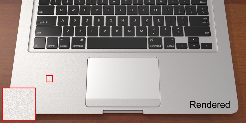
75:2 • Ling-Qi Yan, Miloš Hašan, Bruce Walter, Steve Marschner, and Ravi Ramamoorthi
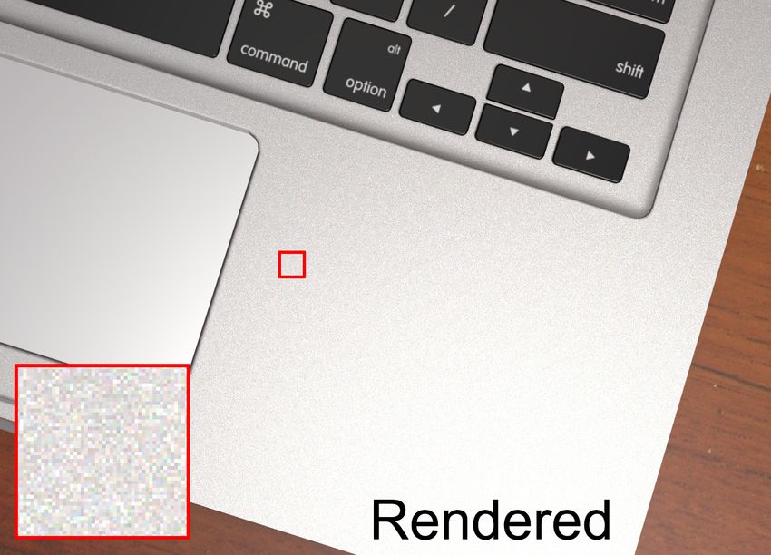
Fig. 2. Left: Rendering of a laptop with a point light and environment lighting using our method. Top right: Close up rendering of the corner of the laptop with
the same lighting condition. Bottom right: A photograph of a MacBook (around 20 cm × 4 cm region) lit by a small LED light in a dark room. Our method is
able to produce appearance that is perceptually similar to the photograph, showing colored glints from the underlying noisy microstructure of the aluminum
laptop body.
heightfield specifying the microgeometry of a surface, how do we our paper is the first to consider this question in full generality,
compute the surface reflection according to laws of physics? modeling the surfaces as arbitrary discretized heightfields.
Most existing solutions either make the approximation of pro- We present an algorithm that can evaluate a spatially varying
viding only a large-area average solution in terms of a mean BRDF BRDF for a given position and incoming/outgoing directions, by
(ignoring spatial detail), or are based on geometric optics (an ap- computing a wave optics reflection integral over the coherence areas
proximation to wave optics), or both. For example, the standard around the position of interest. This requires more computation
microfacet BRDF models commonly used in rendering [Cook and than in the geometric optics solutions, which makes our method
Torrance 1982] assume the surface consists of infinitely small unre- slower, but not prohibitively so; see Table 1. Our solution is based
solved microfacets, which act as perfect mirrors following the rules on approximating the micron-resolution surface wave effects using
of geometric optics. Thus, these models make both of the approxi- Gabor kernels (products of Gaussians with complex exponentials).
mations mentioned (no spatial variation and no wave optics). We use a reciprocal modification of the Harvey-Shack theory in our
Some previous research focused on lifting one or the other of results, but our approach also applies to other wave optics models.
these two limitations. Several wave optics reflection models have We found that the difference between the geometric and wave
been proposed in various areas of physics, including Kirchoff and solution is more dramatic when spatial detail is taken into account.
Harvey-Shack reflection theories [Krywonos 2006], and versions of The visualizations of the corresponding BRDF lobes differ dramati-
these have been used in computer graphics, but always assuming cally, with the sharp folds typical of geometric normal distribution
large-area averages. functions (NDFs) replaced by very different directional patterns
Large-area averages are successful for distant views and smooth il- more akin to laser speckle (Figure 10). The rendered highlights
lumination, but the high-frequency spatially-varying structure seen change appearance, typically with more realistic-looking sharper
in real specular highlights cannot be replicated without modeling peaks and longer tails. Moreover, the wave optics solution varies
discrete, finite microgeometry features. Recent work on rendering as a function of wavelength, predicting noticeable color effects in
glints [Yan et al. 2014, 2016] has moved beyond large-area aver- the highlights (Figure 1). Our results show both single-wavelength
ages, by presenting solutions for surfaces defined by explicit high- and spectral solutions to reflection from common everyday objects,
resolution heightfields (or normal maps). However, these methods such as brushed, scratched and bumpy metals; see the result figures
continue using the rules of geometric optics at scales approaching and supplementary video.
micron resolution, where they are known to become less accurate.
Moreover, recent work has introduced solutions based on wave 2 RELATED WORK
optics that are capable of handling high-resolution surfaces of a We organize the related work into four areas, based on whether they
specific kind, defined by a flat surface with randomly oriented 1D use geometric or wave optics, and whether they target large-area
scratch curves [Werner et al. 2017]. average BRDFs or spatially-varying fine-scale details and “glints”.
This leads to the question: can we design a BRDF model based on
the more accurate wave optics, but also able to compute spatially- Large-area, geometric optics. Microfacet BRDFs have become a
varying solutions with high-resolution detail? To our knowledge, standard tool in rendering [Burley 2012; Butler et al. 2015; Cook and
Torrance 1982; Walter et al. 2007; Westin et al. 2004]. The distribu-
tion of the normals of the microfacets is modeled using a smooth
ACM Trans. Graph., Vol. 37, No. 4, Article 75. Publication date: August 2018.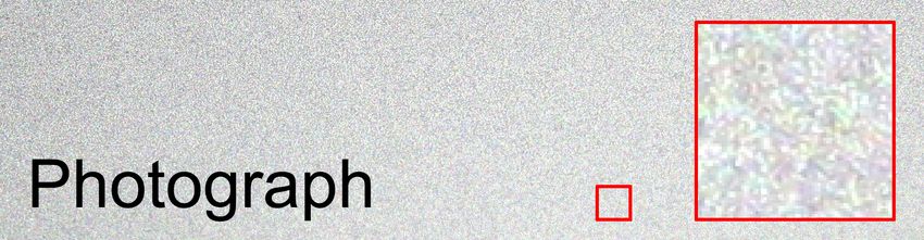
Rendering Specular Microgeometry with Wave Optics •                                  75:3

normal distribution function (NDF), and the BRDF additionally con-             Spatially-varying, wave optics. The only previous work we are
tains Fresnel and shadowing-masking terms. This approach models             aware of in this area is the recent paper by Werner et al. [2017] (with
only directional, not spatial variation; the latter is normally added       a real-time extension by Velinov et al. [2018]), rendering surfaces
by texturing and bump/normal mapping, which has limitations at              with collections of randomly oriented scratches using a Harvey-
high resolutions and under high-frequency lighting. Furthermore,            Shack-based wave optics model. This work represents the surface
geometric optics is theoretically accurate only if surface features         as a collection of one-dimensional scratches over a smooth BRDF.
are locally flat at the scale of microns; many real surfaces violate        Under this assumption, they are able to compute the reflection effi-
this assumption, but empirically the microfacet approach often still        ciently and analytically. In contrast, our method can render arbitrary
provides good results.                                                      heightfields (e.g. Figure 2 and 13), including but not limited to ones
                                                                            containing scratches. Additionally, our scratched heightfields can
   Large area, wave optics. Rough surface reflection models based
                                                                            contain more variety and imperfections, resulting in glinty high-
on wave optics have been heavily studied in physics. Common ap-
                                                                            lights that only roughly align in lines, compared to the smooth line
proximations include Beckmann-Kirchoff theory [Beckmann and
                                                                            highlights of Werner et al (see Figure 1, esp. insets).
Spizzichino 1968] and variations of Harvey-Shack theory[Harvey
1979]; a good overview is the thesis of Krywonos [2006]. In graphics,       3      WAVE BRDF THEORY
wave-based reflection models have been developed for surfaces with
stationary statistics, either random [He et al. 1991] or periodic [Stam     In wave optics, light is described by fields that satisfy appropri-
1999], usually characterized by their power spectral density. A vari-       ate boundary conditions and governing differential equations (e.g.,
ety of methods have been proposed to measure such statistics for            wave or Helmholtz equations). We will consider each wavelength
specific types of real surfaces, especially periodic ones [Dhillon et al.   (denoted λ) separately and use complex-valued fields to encode both
2014; Lanari et al. 2017; Toisoul and Ghosh 2017]. Dong et al. [2015]       magnitude and phase. The local light energy is related to the squared
acquired the surface microgeometry of real metallic surfaces us-            magnitude of the field at that point. Scalar diffraction models, such
ing a profilometer, and applied Kirchhoff theory to successfully            as Harvey-Shack [Krywonos 2006] or Kirchhoff [Ogilvy 1991], can
predict their large scale BRDFs. A combined microfacet-diffraction          be used to estimate the reflected field from a rough surface. Unlike
model was recently proposed by Holzschuch and Pacanowski [2017],            in geometric optics, the contributions from different parts of the
demonstrating better fits to measured BRDF data for some mate-              surface can sum non-linearly due to interference effects, to create
rials than microfacet models alone. Levin et al. [2013] designed            the characteristic diffraction effects of wave optics.
special multi-planar surfaces that can be lithographically fabricated          Let us assume we have a surface heightfield H (s) (as in Figure 3)
to match a target BRDF using wave optics, essentially inverting the         such that for a given 2D point s = [s x , sy ], the corresponding 3D
rendering process.                                                          point on the rough surface is [s x , sy , H (s)]. In our approach, the
   Wave optics has also been used to predict appearance from thin-
film or layered materials (e.g., [Belcour and Barla 2017]), but we                                                                     Light
will only consider single-layer opaque surfaces here. Several meth-                                                                                      ψ
                                                                                                n                                       n                         Sensor
ods support longer-range multi-surface interference effects (e.g.,              Planar                                                         ωi
                                                                                                          H(s)
[Cuypers et al. 2012]), but that is beyond the scope of this paper.             projection S̄                                                                ωo
                                                                                                                                                    ψ̄
   Spatially-varying, geometric optics. Yan et al. [2014; 2016] pre-            Detailed surface S
sented algorithms for rendering glinty surfaces defined by explicit
high-resolution heightfields (or normal maps), under geometric                          Fig. 3. Heightfield surface and BRDF directions example.
optics. These approaches are successful at simulating very high-
resolution, spatially varying glinty behavior. The key idea is to                    i          Imaginary unit for complex numbers, i 2 = −1
extend the NDF from microfacet theory to a patch-based P-NDF,                       λ           Wavelength of light
essentially replacing the large-area average for the whole surface                  n           Average surface normal (equal to z-axis)
by a unique solution per given small patch of the surface. In the first             s           2D point (on the XY plane)
paper, they introduce an algorithm that evaluates P-NDFs by turn-                 H (s)         Height of surface above s
ing the problem into integration over the patch P, finely discretized            H ′ (s)        Gradient of height function
into triangles. The second paper considers the same problem, but                    S̄          Domain of height function (region on XY plane)
proposes a higher-performance algorithm. Instead of discretizing                   AS̄          Area of S̄
the normal map into triangles, they fit small Gaussian elements to                  ωi          Direction from which light arrives (3D unit vector)
texels of the normal map. Our approach is related, but instead of                  ωo           Direction of reflected light (3D unit vector)
real Gaussians, we use complex Gabor kernels, which are better                      ψ           ψ = ωi + ωo
matched to approximating the underlying complex integrals. Jakob                    ψ           2D projection ψ (removing its z-component)
et al. [2014] also simulated glinty surfaces but used a statistical                 fr          Bidirectional reflectance distrib. function (BRDF)
distribution of tiny mirror-like flakes rather than an explicit surface.            F           Surface reflectance (e.g., from Fresnel equations)
In addition to these general approaches, other methods [Bosch et al.            ξ1, ξ2, ξ3      See Figure 6
2004; Mérillou et al. 2001; Raymond et al. 2016] focus specifically
on scratched surfaces, also under geometric optics.                                                         Fig. 4. List of symbols.

                                                                                       ACM Trans. Graph., Vol. 37, No. 4, Article 75. Publication date: August 2018.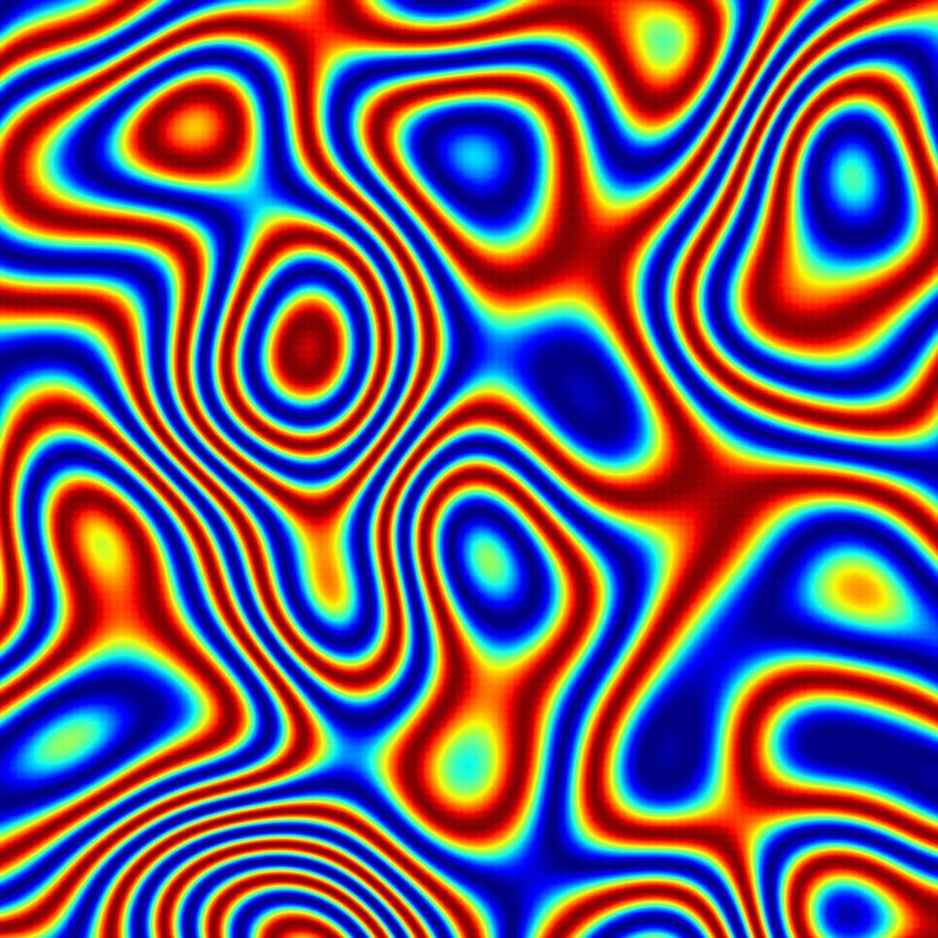
75:4 • Ling-Qi Yan, Miloš Hašan, Bruce Walter, Steve Marschner, and Ravi Ramamoorthi
proxy can be computed using a surface integral of the form:
Z 2
ξ1
R(s) e −i λ (ψ · s ) ds
2π
f r (ωi , ω o ) = (2)
AS̄ S̄
where S̄ is the domain of the heightfield (i.e. the projection of the
rough surface onto the XY plane), AS̄ is its area, and ξ 1 depends on
the chosen diffraction model (see Figure 6) .
The parameters for five different diffraction models are listed in
Figure 6 and detailed derivations of these models are provided in
the supplemental material. These models are closely related and
often produce similar results, especially for low-slope surfaces and
Fig. 5. Left: A discretized surface heightfield at 1 micron resolution, showing paraxial directions. One advantage of our approach is that it can
an area of about 64 × 64 microns. For visualization purposes, we complete the be used to compute any of these models. The first four are derived
heightfield into a continuous function H (s ) by bicubic interpolation. Right: from the Harvey-Shack family of diffraction models [Harvey and
The real component of the reflection function R (s ) of this surface patch, Pfisterer 2016]. The first uses the phase shift approximation from
specifying the spatially varying phase shift. The imaginary component looks Original-Harvey-Shack (OHS) and the second uses the more ac-
similar. curate phase shift from Generalized-Harvey-Shack (GHS). These
produce non-reciprocal BRDFs (i.e. f r (ωi , ωo ) , f r (ωo , ωi )). Recip-
Diffraction Equation Components
rocal BRDF estimates are often preferred in rendering, since real
BRDF Model ξ1 ξ2 ξ3
world BRDFs are reciprocal, and reciprocity also simplifies some
|ωo · n | F light transport algorithms. Therefore we created reciprocal versions
1. OHS λ 2 |ω i · n |
1 2
|ωo · n | F
(R-OHS and R-GHS) by keeping the same planar proxy and phase
2. GHS λ 2 |ω i · n |
1 ψ ·n shift approximations, but using the Kirchhoff propagation integral
2
|ψ · n | F instead of the usual Fourier-based propagation. The fifth model is
3. R-OHS 4λ 2 |ω i · n | |ω o · n |
1 2 equivalent to the Kirchhoff-based BRDF from Dong et al. [2015]
2 and is also reciprocal. In our results we use the third method (R-
|ψ · n | F
4. R-GHS 4λ 2 |ω i · n | |ω o · n |
1 ψ ·n
OHS), with its convenient simplicity and reciprocity, except where
|ψ · n |2 F ψ · H ′ (s ) otherwise noted. In the supplementary material, we include some
5. Kirchhoff 4λ 2 |ω i · n | |ω o · n |
1− ψ ·n ψ ·n
comparisons using the other models, showing that (for computer
Fig. 6. BRDF integrals for five scalar diffraction models (see equations (1) graphics purposes) the results are often quite similar.
and (2)). The first two are based on the Original-Harvey-Shack (OHS) and
the Generalized-Harvey-Shack (GHS) models. The next two are reciprocal 3.1 Coherence area
versions of these models we created by substituting Kirchhoff propagation The spatial size over which the incident light’s phase remains cor-
instead of Fourier: Reciprocal OHS (R-OHS) and Reciprocal GHS (R-GHS). related (i.e. coherent) is known as its coherence area. Equation 2
The fifth is a fully Kirchhoff-based BRDF model. Detailed derivations of
was derived using incident light with an infinite coherence area, but
these models can be found in the supplemental material.
realistic sources have finite ones (typically inversely related to their
solid angle [Mandel and Wolf 1995]). For example, sunlight [Mashaal
heightfield is typically discretized at the resolution of 1 µm per et al. 2012] has a measured coherence area diameter of roughly one
texel. Figure 5 (left) illustrates a small example heightfield. Our goal hundred wavelengths, or ∼ 50 microns.
is to estimate the surface’s Bidirectional Reflectance Distribution Coherent contributions must be summed using their complex
Function (BRDF) f r (ωi , ω o ), which is defined as the ratio between field values, while incoherent ones are accumulated by summing
the reflected radiance in direction ωo and the incident irradiance their energy (or equivalently, averaging their BRDF values). This
from direction ωi . Light reflecting from different parts of the surface is commonly simulated (e.g., [Dong et al. 2015; Levin et al. 2013;
will travel different distances depending on the local surface height. Werner et al. 2017]) by spatially limiting the surface integrals using
This causes phase shifts in reflected waves which then interfere a coherence kernel w (s), and then averaging multiple such BRDF
with each other to determine the BRDF. evaluations over the region of interest (e.g., the pixel footprint). The
These phase shifts can be approximated using a planar surface principal effect of limiting the coherence area is a small angular
that reflects light with a spatially-varying phase shift, specified by blurring of the BRDF. The BRDF estimate for one coherence area
its reflection function: becomes:
2π
ξ 3 H (s )
R(s) = ξ 2 e −i λ . (1) ξ1
Z 2
R ⋆ (s) e −i λ (ψ · s ) ds
2π
f r (ωi , ωo ) = (3)
Figure 5 (right) shows a visualization of the real component of this Ac S̄c
function. The values of ξ 2 and ξ 3 depend on which diffraction model R ⋆ (s) = w (s −x c )R(s) (4)
is chosen (see Figure 6 for examples). We represent the directions
ωi and ω o as 3D unit vectors. Let ψ = ω i + ω o and ψ be its 2D where S̄c is the portion of S̄ within the support of the coherence
projection (by discarding its z-component). The BRDF of this planar kernel centered at x c , the corresponding normalization factor is
ACM Trans. Graph., Vol. 37, No. 4, Article 75. Publication date: August 2018.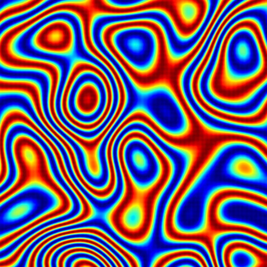
Rendering Specular Microgeometry with Wave Optics •                                      75:5

Ac = |w (s)| 2 ds, and R ⋆ is the product of R(s) and the coherence               4.1   Gabor kernels
      R

kernel. This has the advantages of limiting our integrals to small                Let us define a Gabor kernel as the product of a 2D Gaussian and a
surface regions and effectively prefiltering the BRDF to remove                   complex exponential:
high frequency angular features that we expect are too small to
be resolved. Generally we do not need to exactly match the real                                 д(s; µ, σ , a) = G 2D (s; µ, σ ) e −i2π (a · s )       (7)
coherence area. Overestimating it leads to high angular frequency
                                                                                                                           ∥ s −µ ∥ 2

aliasing that can be resolved by using more light samples, while                  where G 2D (s; µ, σ ) = 2π1σ 2 exp − 2σ 2            is a normalized 2D
underestimating it causes some angular over-blurring of the BRDF.                 isotropic Gaussian. Here µ is the center, σ the width and a the
   During rendering, rather than trying to estimate each source’s                 plane wave parameter. This definition is similar to others used in
coherence area, we use a fixed size, which should be at least as large            the literature; the normalization constant of the Gaussian and the ad-
as for any expected light source. For w we use a Gaussian with                    ditional 2π factor in the complex exponential are chosen to simplify
standard deviation of 10 microns (similar to [Werner et al. 2017]).               the following derivations.
                                                                                     The Fourier transform of a Gabor kernel can be written as another
3.2    Fourier Interpretation                                                     Gabor kernel:
                                                                                      F [д(s; µ, σ , a)](v) = e −i2π ( µ · (v +a ) ) e −2π σ ∥v +a ∥
                                                                                                                                           2 2       2
Let us denote the Fourier transform of a 2D function f (s) as:
                                                                                                                 1 −i2π (µ · a )                 1
                                                                                                            =        e                 д  v; −a,       , µ   (8)
                                        Z
            F [f ] (v) ≡ fH(v) ≡                 f (s) e −i2π (s · v ) ds   (5)                               2πσ 2                              2πσ
                                            R2
                                                                                  4.2   Approximating R with Gabor kernels
where v is a 2D frequency vector. Equation (3) can be rewritten as:               We first subdivide the heightfield domain S̄ into a grid of cells.
                                                                                  We use a uniform grid so all the cells are identically-sized squares,
                                        ξ 1 f⋆ ψ 2
                                                 !
                    f r (ωi , ω o ) =       R                               (6)   matching the original heightfield texels, but an adaptive subdivision
                                        Ac     λ                                  could also be used. Then we select a set of cells, with centers mk ,
                                                                                  that covers the support of the current coherence kernel. Since the
Thus the BRDF can be computed using the Fourier transform of                      cells are much smaller than the coherence area, we approximate
R ⋆ (s) evaluated at ψ/λ. One approach could be to compute and store              the coherence kernel as being constant over a cell with value w k =
the full Fourier transform, either analytically or numerically via the            w (mk − x c ). Then we place a Gabor kernel centered on each grid
Fast Fourier Transform (FFT) algorithm. However we use tabulated                  cell designed to approximate R(s) in its neighborhood. Together
heightfields which have no simple analytic Fourier transform, and                 this gives us an approximation for R ⋆ (s) of the form:
precomputing FFTs for each surface position would require far too                                    X              X
much storage. Computing full FFTs at render time would also be very                        R ⋆ (s) ≈   w k Rk (s) =    w k Ck д(s; mk , σk , ak )    (9)
inefficient as we typically only need one, or at most a few, values                                    k                    k
for each BRDF evaluation. Also R ⋆ (s) typically contains very high               where Ck is a complex constant, incorporating an appropriate scal-
frequencies, much higher than those in the original heightfield, so               ing coefficient and phase shift.
using an FFT would require an extremely fine discretization step of                  We choose σk = lk /2, where lk is the side length of the cell.
0.1 microns or less. We could evaluate just Rf⋆ (ψ/λ) as needed using             This choice was found to give good results experimentally. A sum
numerical quadrature, but this would similarly be expensive and                   of Gaussians is not an exact partition of unity; this leads to slight
require high sampling rates. However, we do use the FFT approach                  approximation error that manifests itself as spurious periodic copies
as a ground truth for checking the correctness of our approach in                 of the main transform image in the Fourier domain. However, for
Section 6.                                                                        the choice σk = lk /2, the copies are weak enough that we do not
                                                                                  observe them in practice.
4     EFFICIENT BRDF EVALUATION                                                      Next, we approximate the heightfield H (s) in each cell by its first
In this section, we discuss how to evaluate the BRDF integrals for our            order expansion around mk :
wave optics diffraction models. Our high-level idea for efficiently                           H (s) ≈ H (mk ) + H ′ (mk ) · (s − mk )                                        (10)
approximating the integral in equation (3) is to approximate the                                           ′                                    ′
                                                                                                     = H (mk ) · s + H (mk ) − H (mk ) ·mk

                                                                                                                                                                             (11)
phase-delay reflection function R ⋆ (s) by a weighted combination of
Gabor kernels, which are products of a 2D Gaussian with a complex                 where H ′ (m k ) is the gradient of the heightfield at mk . Substituting
exponential (plane wave). These kernels are well suited to repre-                 this approximation into the definition of R(s), we can approximate
senting the high-frequency features found in typical R ⋆ (s), while               a single grid cell’s contribution as:
also having other desirable properties.                                                                                          i 2π ξ 3
                                                                                                                                            H (s )
   Notably, Gabor kernels have an analytical Fourier transform that                        Rk (s) = B 2D (s; mk , lk ) ξ 2 e −      λ                                        (12)
is itself a Gabor kernel. This means that the kernels and their trans-                                                                i 2π ξ

                                                                                                                                     − λ 3         α k +H ′ (m k ) · s
forms both have spatially localized support (ignoring negligibly                                   ≈ lk2 G 2D (s; µ k , σk ) ξ 2 e                                           (13)
small values of the Gaussian component), which is a key property                  where α k = H (mk ) − H ′ (mk ) ·mk . B 2D is a binary box function
for designing an efficient pruning algorithm.                                     indicating the domain of the grid cell, which integrates to the cell’s

                                                                                         ACM Trans. Graph., Vol. 37, No. 4, Article 75. Publication date: August 2018.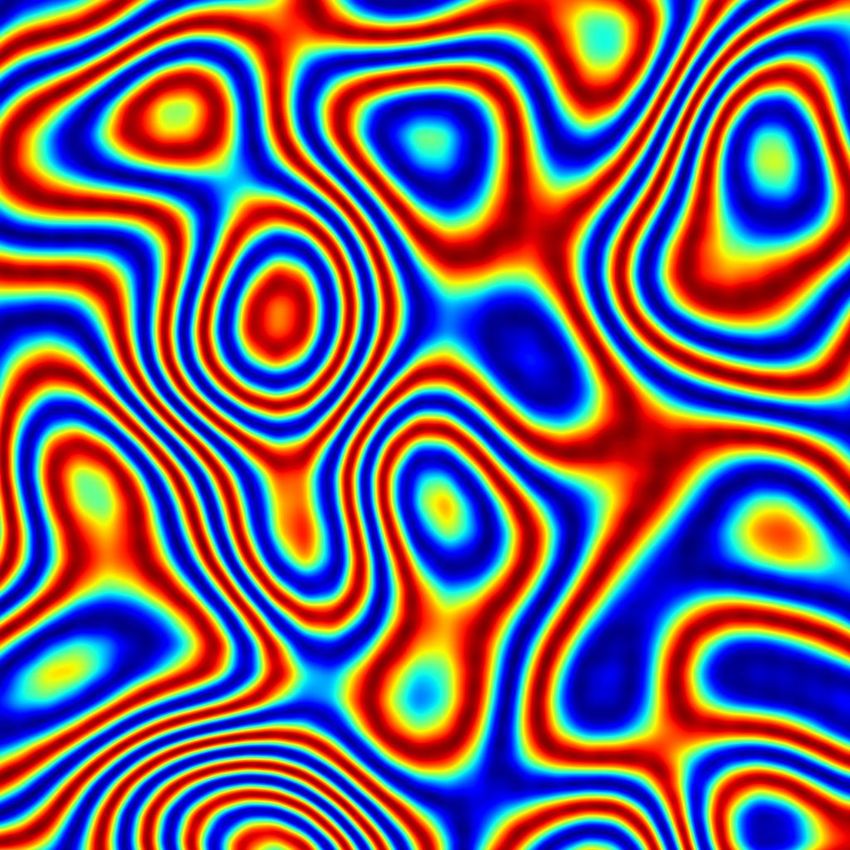
75:6 • Ling-Qi Yan, Miloš Hašan, Bruce Walter, Steve Marschner, and Ravi Ramamoorthi

                                                                                                Appendix A briefly sketches an alternate derivation of our method
                                                                                              where the surface is approximated by overlapping planar elements.

                                                                                              5   IMPLEMENTATION
                                                                                              In this section, we provide key implementation details of our Gabor
                                                                                              kernel solution.
                                                                                                 Heightfields and Gabor kernels. We use pre-defined high resolu-
      ground truth               2x2 kernels / texel                    1 kernel / texel
                                                                                              tion (8K × 8K) heightfields as texture maps to specify the microge-
                                                                                              ometry, where each texel represent a fixed size of 1 square micron
                                                                                              in the real world. The heightfields are tiled repeatedly to achieve
                                                                                              a high resolution over a surface. The texels in a heightfield form
                                                                                              a uniform grid naturally, so, we convert each texel into a Gabor
                                                                                              Kernel, as specified in Sec. 4.
                                                                                                 For simplicity, we assume no distortion from the texture map,
                                                                                              i.e. the texture coordinates are defined to be area preserving and
 1 kernel / 2x2 texels 1 kernel / 4x4 texels 1 kernel / 8x8 texels                            orthogonal in terms of u and v directions in the world coordinate
                                                                                              system.
Fig. 7. A color-mapped (range [-1,1]) visualization of the real component
of R (s ) for the isotropic noise heightfield (the imaginary component looks
                                                                                                 Acceleration by pruning. To accelerate computation, the key is
similar). The area depicted is about 64 × 64 texels, using the resolution                     to quickly decide whether a Gabor kernel contributes to the de-
of 1 micron / texel. Note the common structure seen in these functions:                       sired outgoing direction ωo . Regardless of the cancellation from
high-frequency ripples aligned with slopes of the original heightfield, with                  the complex numbers, each Gabor kernel is bounded by a Gaussian
frequency increasing proportional to slope. This structure is ideal for approx-               G 2D (s; mk , σk ) positionally and by G 2D (v; −ak , 2π1σk ) direction-
imation by Gabor kernels. These images show the approximation quality                         ally. Although in theory Gaussians have infinite support, in practice
for various kernel sampling densities. All our results use 1 kernel per texel                 we limit them to within ±3 standard deviations, and clamp them to
(i.e. per micron). Note that as the number of kernels decreases, the approxi-                 zero outside this region so they have only localized support.
mation degrades, as expected.
                                                                                                 We pre-generate a mipmap-style hierarchy for each heightfield,
                                                                                              where each node contains both positional and directional bounding
area lk2 . Then we replace the box function with a 2D Gaussian of                             boxes of its 4 child nodes. For each BRDF query, we perform a
the equal area.                                                                               top-down traversal of this hierarchy, discarding nodes that are not
  Comparing Eqn. 13 with the definition in Eqn. 9, we have                                    within the coherence region S̄ using their positional bounding boxes.
                                    i 2π ξ 3                                                  At the same time, we use the directional bounding boxes to prune

                                                   H (m k )−H ′ (m k ) · m k
                  Ck = lk2 ξ 2e −      λ                                               (14)
                                                                                              the nodes that will not contribute to the query direction ψ/λ.
                     ξ 3 H ′ (mk )                                                               Figure 9 shows the number of evaluations towards different direc-
                  ak =                                          (15)                          tions to generate an example BRDF image. In general, each Gabor
                           λ
which completes our Gabor approximation for R ⋆ (s).                                          kernel contributes to a much larger range directionally in wave
  Figure 7 shows R(s) for an example heightfield compared to its                              optics than the elements in geometric optics [Yan et al. 2016]. This
approximation as a sum of Gabor kernels. At the density of 1 kernel                           explains the soft appearance in these images, as well as slower per-
per texel, though the sampling pattern is just visible, we obtain a                           formance of wave optics. However, our hierarchical pruning is still
sufficiently good approximation that reproduces the relevant details.                         efficient. In practice, we have a more than 50× speedup as compared
                                                                                              to the un-accelerated implementation.
4.3    BRDF approximation                                                                        Importance sampling. With the Gabor kernels defined to represent
Finally we use our Gabor kernel approximation to evaluate the                                 a heightfield, it is straightforward to perform BRDF importance
BRDF. Starting from Equation 6 we have:                                                       sampling to get the outgoing ray for global illumination. First, we
                      ξ 1 f⋆ ψ 2
                                !                                                             randomly pick a Gabor kernel within the coherence region according
    f r (ωi , ω o ) =     R                                     (16)                          to its weighting function w (s). Then, we immediately know that
                      Ac     λ
                                                                                              the chosen Gabor kernel contributes to a Gaussian directionally, as
                                                             !2                               analyzed in the acceleration part. By sampling this Gaussian, we
                      ξ1 X                                 ψ
                    ≈       w k Ck F [д(s; mk , σk , ak )]      (17)                          have the sampled query direction ψ/λ and thus the corresponding
                      Ac                                   λ
                             k                                                                outgoing direction ωo .
where we can use the above definitions of the quantities Ck and                                  The sampling weight can be calculated as the BRDF evaluation
ak , and equation (8) to evaluate the Fourier transform of the Gabor                          with sampled ωo , divided by the sampling pdf. However, in practice,
kernel. Thus we can evaluate the sum in a straightforward manner                              we found that wave optics effects are essentially not observable
by iterating over all the cells within the coherence area. We also                            in indirect lighting. So, we assume that our sampling weight is
apply pruning to non-contributing cells, as detailed in Section 5.                            always 1, i.e. discarding the complex cancellations and assuming

ACM Trans. Graph., Vol. 37, No. 4, Article 75. Publication date: August 2018.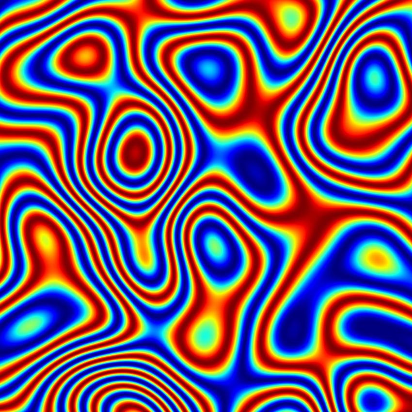
Rendering Specular Microgeometry with Wave Optics •                         75:7

Fig. 8. The heightfields used in this paper. Left to right: isotropic bumps, brushed metal, scratched metal. These are 5122 crops of the full 81922 maps. The
units (horizontal and vertical) are microns (µm), so the full maps cover a square area about 8.2 mm × 8.2 mm large.

                                                                                  number of spectrum samples, which gives us another 3× speedup,
                                                                                  compared with brute force spectral rendering.

                                                                                  6 RESULTS
                                                                                  6.1 Heightfield and BRDF visualizations
                                                                                  Figure 8 shows a color-mapped visualization of the heightfields used
                                                                                  in our results. For all heightfields, we use a discretization step of 1
                                                                                  micron. The heightfields were generated procedurally by inverse
     # evaluations (isotropic)           # evaluations (brushed)                  FFT noise generation, and (in the case of scratches) by drawing lines
                                                                                  with randomized positions, depths, and widths.
Fig. 9. Visualization of the numbers of Gabor kernels that are evaluated to          In Figure 10, we show visualizations of the outgoing BRDF lobes of
calculate the BRDF values toward different directions. Note that the shapes
                                                                                  our model and geometric optics, for a fixed incoming direction and
of the corresponding BRDFs are captured well, and that a large number of
evaluations are successfully pruned.
                                                                                  footprint (coherence area). This illustrates the differences between
                                                                                  geometric and wave optics, and also the differences between a single-
                                                                                  wavelength and spectral simulation. Note that the appearance of
contribution only from the Gaussian part of each Gabor kernel. This
                                                                                  high-frequency features is clearly different in the geometric and
gives us significant speed-up, allowing the indirect illumination
                                                                                  wave solutions: the geometric solutions contain sharp folds in areas
to use more samples to converge. This is roughly equivalent to
                                                                                  where the normal map Jacobian becomes singular [Yan et al. 2014].
reducing the coherence area used for indirect illumination to the
                                                                                  The wave optics solutions have no such features, and the high
size of our Gabor kernels.
                                                                                  frequencies in them are more reminiscent of laser speckle. Also note
   Practical rendering pipeline. For convenience, we separate the final           the significant color effects in the full spectral wave optics version.
rendered image into three components. First, direct illumination                     In Figure 11, we show BRDF lobes computed with our approach
from point lights. Second, indirect illumination from point lights.               (for a single wavelength) side-by-side with lobes computed using the
Third, illumination from other lights, including the environment                  FFT algorithm applied to equation 6. Note the close match, despite
lighting, both direct and indirect. The separation allows us to use               our method taking a completely different approach of Gabor kernel
very few samples per pixel to render the most time-consuming first                approximation.
part, usually only 4 to 25 samples on a regular sub-pixel grid.
   Spectral rendering. For each BRDF evaluation, we compute for                   6.2   Rendered results
different wavelengths ranging from 0.36 microns to 0.83 microns,                  In this section, we illustrate our method’s capability to render actual
i.e. the visible spectrum. We find that using 8 spectral samples is               scenes using wave optics, as shown in Figures 1, 2, 12, and 13. To
generally good enough to produce identical results to those gener-                show that the results computed separately at each frame are tempo-
ated using more samples. We split the wavelength range into bins                  rally coherent, please see the accompanying video. We implement
and use the midpoints (not endpoints) of the bins as the samples.                 our method using Mitsuba [Jakob 2010], and run all renderings in
We follow the standard spectrum samples→XYZ→RGB method to                         720p (1280 × 720) on a 6-core Intel i7-4770K desktop at 3.5 GHz,
eventually convert the spectral values to the sRGB color space.                   hyperthreaded to 12 threads.
   We also find it useful to perform the top-down pruning only once                  Scene configurations and performance comparisons are listed in
using the largest wavelength. In this way, we record all contributing             Table 1. In general, for direct illumination from point lights, our
Gabor kernels first, then evaluate them for all spectrum samples at               method with a single wavelength is about 5 − 20× slower than geo-
once. As a result, our computation time scales sub-linearly with the              metric optics, and about another 3.5× slower with 8 spectral samples.

                                                                                         ACM Trans. Graph., Vol. 37, No. 4, Article 75. Publication date: August 2018.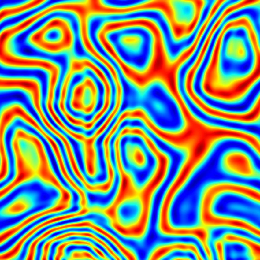
75:8 • Ling-Qi Yan, Miloš Hašan, Bruce Walter, Steve Marschner, and Ravi Ramamoorthi

                                                                                 Table 1. Scene configurations including materials of the main objects and
                                                                                 number of samples per pixel, and performance comparisons between geomet-
                                                                                 ric optics and wave optics with 1 and 8 spectral samples. For the performance
                                                                                 of the Patch scene, we use the isotropic noise heightfield as representative.

                                                                                   Scene                       Patch     Cutlery     Laptop     Tumbler
                                                                                   # Point light(s)               1         1           1           2
                                                                                   # Env. light                   0         1           1           1
                                                                                   Material                      Al        Ag          Al          Fe
                                                                                   # Samples (direct)             4         9          25          25
                                                                                   # Samples (ind.+env.)        N/A        256        1024        1024
                                                                                   Direct (geom.)               9.6s      3.1s        37.4s      19.8s
                                                                                   Direct (single)              3.7m      0.8m        6.4m       1.9m
                                                                                   Direct (spectral)           13.1m      2.4m       21.1m       6.4m
                                                                                   Indirect + env.              N/A       4.0m       25.1m       9.7m
                                                                                   All (geom.)                  N/A       4.2m       25.7m       10.0m
                                                                                   All (single)                 N/A       4.8m       31.5m       11.6m
                                                                                   All (spectral)               N/A       6.4m       46.2m       16.1m

                                                                                 of the brushes and scratches to make them more visible under the
                                                                                 point light.
                                                                                    From these images, we can clearly see that our method is able to
        geometric                    single                      spectral        produce characteristic structures from the underlying heightfields:
          optics                   wavelength                                    intuitively, round highlight for isotropic, vertical anisotropic high-
                                                                                 light for brushed and spiderweb-like highlight for scratched. These
Fig. 10. Visualizations of the outgoing BRDF lobes on the projected hemi-        shapes indicate the correctness of our method. Also, since different
sphere. Top: isotropic bumps, middle: brushed, bottom: scratched. Note the       wavelengths behave differently in wave optics, colors are expected
clearly different high-frequency features predicted by geometric and wave        from spectral rendering.
optics. Also note the significant color effects predicted by wave optics (here
we are using 8 spectral samples).                                                   Cutlery. This scene shows silver cutlery with strong scratches,
                                                                                 rendered using a point light with static grayscale environment light-
                                                                                 ing, in order to make sure that the colors are from diffraction. In
                                                                                 Figure 1, we can clearly see the colored scratches rendered using
                                                                                 multiple wavelengths. Also, even with a single wavelength, our
                                                                                 method is able to generate a more convincing result, as we com-
                                                                                 pare with the geometric method by Yan et al. [2016]. The geometric
           isotropic bumps                              brushed metal            method arguably produces harsher glints, due to the sharper folds
                                                                                 in the BRDF lobes predicted by the P-NDF theory.
Fig. 11. Comparison of BRDF lobes computed using our Gabor kernel ap-               In the video, we move the point light back and forth, so that we
proach (left image in each pair) to ground truth computed by evaluating          can see the scratches and highlights changing consistently. We also
equation 6 using the FFT algorithm (right image).                                compare with geometric optics. We can clearly see strong cross-
                                                                                 shaped highlights from geometric optics, but they’re more subtle in
This is because of the wide directional spread predicted by wave                 wave optics.
optics, as analyzed in Section 5. However, direct illumination only
                                                                                    Laptop. This scene shows a laptop with a roughened aluminum
takes up about half of the overall computing time. Considering indi-
                                                                                 matte finish (modeled as a Gaussian random heightfield). It is ren-
rect lighting and environment lighting together, the performance of
                                                                                 dered using a point light and environment lighting. We can observe
our wave optics method is within 1.5× of geometric optics, and is
                                                                                 colored glints in Figure 2. Albeit subtle, these colored glints are
thus a practical solution. In the rest of this section, we will discuss
                                                                                 pervasively observed in the real world. To further verify this effect,
individual scenes.
                                                                                 we illuminated a MacBook using an LED light from a cell phone in
  Patch. This is a simple scene showing a 5 cm × 5 cm patch. The                 a dark room; this leads to obvious colored highlights. Our method
camera is looking towards the center of the patch from an elevation              is able to produce perceptually similar appearance.
angle of 45◦ . The point light is on the opposite side, and moves left              In the video, we move the light to show how the colored glints
and right in the video. Figure 12 shows renderings of three different            change. We also show comparisons with geometric optics, which
heightfields (isotropic noise, brushed and scratched), each rendered             produces much more “noisy” glints. This can also be observed from
using multiple wavelengths, single wavelength (0.4 microns) and                  the BRDF images in Figure 10, where geometric optics preserves
geometric optics for comparison. We added isotropic noise on top                 every detail from the heightfield, including sharp edges and corners,

ACM Trans. Graph., Vol. 37, No. 4, Article 75. Publication date: August 2018.
Rendering Specular Microgeometry with Wave Optics •                        75:9

                                                                             in Figure 13, our method is able to handle the anisotropic appear-
                                                                             ance, resulting in two vertical lines of highlights. From the insets,
                                                                             we can also see that the geometric method generates wider highlight
                                                                             peaks but narrower highlights overall, while our method is able to
                                                                             produce thin peaks but with much wider spread. This observation
                                                                             corresponds to the brushed BRDF images in Figure 10, where most
                                                                             energy concentrates in the central vertical line for wave optics. A
                                                                             similar observation was noted by Dong et al. [2015]. Moreover, the
                                                                             observation is also in accordance with the geometric GGX BRDF
                                                                             [Walter et al. 2007], well known for its “long tail” and its ability
                                                                             to better represent slow falloffs of highlights than other geometric
                                                                             BRDFs such as Beckmann. The question of why wave optics often
                                                                             leads to longer tails is complex; a simple though incomplete expla-
                                                                             nation is that wave optics is less influenced by finer scale roughness,
                                                                             leading to sharper peaks, while off-peak dropoff depends on de-
                                                                             structive interference which tends to be somewhat random and
                                                                             incomplete, leading to stronger tails.

                                                                                Limitations and future work. Currently our approach only looks
                                                                             at single specular reflection, ignoring inter-reflection, layered mate-
                                                                             rials, refraction, or complex 3D structures (e.g., in biological irides-
                                                                             cence). Our computational expense currently requires separation of
       isotropic                brushed                scratched             direct illumination due to small lightsources from other components,
                                                                             and using a different (cheaper) BRDF for these components; further
Fig. 12. The Patch scene showing renderings of different heightfields with   accelerations should be explored. Improved importance sampling
a point light. (Top row) Spectral. (Middle row) Single wavelength. (Bottom   techniques would also help. Physical measurement to acquire the
row) Geometric.                                                              heightfields would be another interesting addition.

                                                                             7    CONCLUSION
                                                                             As computer graphics has pursued ever increasing realism in mate-
                                                                             rial appearance, there has been a trend from strictly using geometric
                                                                             optics to introducing wave optics in the derivation of BRDF models
                                                                             and in the simulation of specific iridescence effects. In this paper we
                                           Wave               Wave           have taken this process to a new level, introducing the first practical
                                           optics             optics
                                                                             technique for simulating full diffraction effects in completely arbi-
                                                                             trary micron-scale height-field geometry. The result is a dramatic
                                                                             change in the predicted BRDF due to reflection from small areas of
                                                                             surface: the unrealistically sharply defined structures of geometric
                                                                             optics give way to softer results that depend on wavelength, intro-
                                                                             ducing color into the BRDF. In practice, the new model produces
                                          Geometric         Geometric
                                                                             softer, more natural looking reflections from microgeometry, with
                                           optics            optics          subtle color effects visible under sharp lighting.
                                                                                BRDF models that are derived from wave optics predict differ-
          full rendering              dir.+ind.+env. dir. illum. only
                                                                             ent appearance than microfacet models, but the results can often
                                                                             be nearly matched by microfacet models with somewhat different
Fig. 13. The Tumbler scene rendered with two point lights and environment
                                                                             parameters. In the case of surface detail, the geometric model will al-
lighting, showing brushed aluminum with strong anisotropy. Insets compare
our spectral method (top row) with the geometric method (bottom row).        ways predict reflection patterns with hard edges induced by folds in
We can see that the geometric method produces wider highlight peaks but      the set of reflected rays. Here moving to wave optics—the model ap-
narrower highlights overall, and misses the colored glints.                  propriate to the scale in question—produces fundamentally different
                                                                             results, with smooth highlight edges and color effects.
                                                                                An exciting implication of our work is that it provides the ability
while wave optics smooths the details out. This is also expected in
                                                                             to represent surface features at all scales with the appropriate type
theory, because wave optics tells us that the light will “ignore” struc-
                                                                             of model: large features can be handled with geometry; smaller
tures whose sizes are comparable or smaller than the wavelength.
                                                                             ones down to a fraction of a millimeter can be represented using
  Tumbler. This scene illustrates a tumbler with brushed metal on            geometric normal maps; and features down to wavelength scale
the body under two point lights and environment lighting. As shown           are represented as diffracting height fields. Smaller features than

                                                                                     ACM Trans. Graph., Vol. 37, No. 4, Article 75. Publication date: August 2018.
75:10 •       Ling-Qi Yan, Miloš Hašan, Bruce Walter, Steve Marschner, and Ravi Ramamoorthi

that are not optically relevant and are not needed in any visual                             Boris Raymond, Gael Guennebaud, and Pascal Barla. 2016. Multi-Scale Rendering
simulation. Though the speed and memory footprint of our initial                                of Scratched Materials using a Structured SV-BRDF Model. ACM Transactions on
                                                                                                Graphics (July 2016). https://doi.org/10.1145/2897824.2925945
implementation can be further reduced in future work, our method                             Jos Stam. 1999. Diffraction Shaders. In SIGGRAPH 99. New York, NY, USA, 101–110.
is already efficient enough to use routinely in offline rendering. We                           https://doi.org/10.1145/311535.311546
                                                                                             Antoine Toisoul and Abhijeet Ghosh. 2017. Practical Acquisition and Rendering of
can represent the appearance of rough surfaces with no excuses                                  Diffraction Effects in Surface Reflectance. ACM Trans. Graph. 36, 5, Article 166 (July
about wave effects being assumed irrelevant or surface details being                            2017), 16 pages. https://doi.org/10.1145/3012001
left out of the model.                                                                       Zdravko Velinov, Sebastian Werner, and Matthias B. Hullin. 2018. Real-Time Rendering
                                                                                                of Wave-Optical Effects on Scratched Surfaces. Computer Graphics Forum 37 (2)
                                                                                                (Proc. EUROGRAPHICS) 37, 2 (2018).
ACKNOWLEDGEMENTS                                                                             Bruce Walter, Stephen R. Marschner, Hongsong Li, and Kenneth E. Torrance. 2007.
                                                                                                Microfacet Models for Refraction Through Rough Surfaces (EGSR 07). 195–206.
We thank the reviewers for many helpful suggestions. This work was                           Sebastian Werner, Zdravko Velinov, Wenzel Jakob, and Matthias B. Hullin. 2017. Scratch
supported in part by NSF grant IIS-1703957, grants from Autodesk,                               Iridescence: Wave-optical Rendering of Diffractive Surface Structure. ACM Trans.
an NVIDIA Fellowship, the Ronald L. Graham endowed Chair, and                                   Graph. 36, 6, Article 207 (2017), 14 pages. https://doi.org/10.1145/3130800.3130840
                                                                                             Stephen H Westin, Hongsong Li, and Kenneth E Torrance. 2004. A comparison of four
the UC San Diego Center for Visual Computing.                                                   brdf models. In Eurographics Symposium on Rendering. pags. 1–10.
                                                                                             Ling-Qi Yan, Miloš Hašan, Wenzel Jakob, Jason Lawrence, Steve Marschner, and Ravi
REFERENCES                                                                                      Ramamoorthi. 2014. Rendering Glints on High-resolution Normal-mapped Specular
                                                                                                Surfaces. ACM Trans. Graph. 33, 4, Article 116 (2014), 9 pages. https://doi.org/10.
P. Beckmann and A. Spizzichino. 1968. The Scattering of Electromagnetic Waves                   1145/2601097.2601155
    from Rough Surfaces. Books on Demand. http://books.google.com/books?id=                  Ling-Qi Yan, Miloš Hašan, Steve Marschner, and Ravi Ramamoorthi. 2016. Position-
    nn92AAAACAAJ                                                                                normal Distributions for Efficient Rendering of Specular Microstructure. ACM Trans.
Laurent Belcour and Pascal Barla. 2017. A Practical Extension to Microfacet Theory              Graph. 35, 4, Article 56 (2016), 9 pages. https://doi.org/10.1145/2897824.2925915
    for the Modeling of Varying Iridescence. ACM Trans. Graph. 36, 4, Article 65 (July
    2017), 14 pages. https://doi.org/10.1145/3072959.3073620
Carles Bosch, Xavier Pueyo, Stéphane Mérillou, and Djamchid Ghazanfarpour. 2004. A           A     ALTERNATE METHOD DERIVATION
    Physically-Based Model for Rendering Realistic Scratches. In Computer Graphics
    Forum, Vol. 23. Wiley Online Library, 361–370.                                           Here we briefly sketch an alternative, but mathematically equiva-
Brent Burley. 2012. Physically-Based Shading at Disney. Technical Report (2012).             lent, derivation of our method. One can also view our method as
Samuel D Butler, Stephen E Nauyoks, and Michael A Marciniak. 2015. Comparison of
    microfacet BRDF model to modified Beckmann-Kirchhoff BRDF model for rough                approximating the rough surface by a set of small planar elements,
    and smooth surfaces. Optics Express 23, 22 (2015), 29100–29112.                          or flakes, with one per grid cell. These flakes have soft overlap-
R. L. Cook and K. E. Torrance. 1982. A Reflectance Model for Computer Graphics. ACM          ping boundaries in S̄, defined by a Gaussian flake shape function
    Trans. Graph. 1, 1 (1982), 7–24.
Tom Cuypers, Tom Haber, Philippe Bekaert, Se Baek Oh, and Ramesh Raskar. 2012.               K (s) = lk2 G 2D (s; 0, σk ), which assuming a uniform grid, is the same
    Reflectance Model for Diffraction. ACM Trans. Graph. 31, 5 (2012), 122:1–122:11.         for all flakes. K is normalized so that its integral is equal to the grid
Daljit Singh Dhillon, Jeremie Teyssier, Michael Single, Michel Milinkovitch Iar-
    solav Gaponenko, and Matthias Zwicker. 2014. Interactive Diffraction from Bi-
                                                                                             cell area. The flakes are centered at the grid cell centers mk .
    ological Nanostructures. Computer Graphics Forum 33, 8 (2014), 177–188. https:              Approximating the coherence kernel as constant over a flake with
    //doi.org/10.1111/cgf.12425                                                              w k = w (mk −x c ), and evaluating Equation (3) as a sum over the
Zhao Dong, Bruce Walter, Steve Marschner, and Donald P. Greenberg. 2015. Predicting
    Appearance from Measured Microgeometry of Metal Surfaces. ACM Trans. Graph.              flake approximation of the surface gives:
    35, 1, Article 9 (2015), 13 pages. https://doi.org/10.1145/2815618                                                      Z                                       2
James Harvey. 1979. Fourier treatment of nearâĂŘfield scalar diffraction theory. Amer-                              ξ1 X
                                                                                                                                  K (s −mk )R(s) e −i λ (ψ · s ) ds
                                                                                                                                                      2π
    ican Journal of Physics 47, 11 (1979), 974–980. https://doi.org/10.1119/1.11600              f r (ωi , ωo ) ≈        wk                                           (18)
James E. Harvey and Richard N. Pfisterer. 2016. Evolution of the transfer function                                  Ac        S̄c
                                                                                                                       k
    characterization of surface scatter phenomena. Proc.SPIE 9961 (2016), 9961 – 9961 –
    17. https://doi.org/10.1117/12.2237083                                                   Then we can expand R(s) using (1), substitute the per-flake planar
Xiao D. He, Kenneth E. Torrance, François X. Sillion, and Donald P. Greenberg. 1991. A       height approximation, H (s) = H (mk )+H ′ (mk ) · (s − mk ), and after
    Comprehensive Physical Model for Light Reflection. SIGGRAPH Comput. Graph. 25,
    4 (1991), 175–186. https://doi.org/10.1145/127719.122738                                 some rearranging of terms, recognize that the integral has the form
Nicolas Holzschuch and Romain Pacanowski. 2017. A Two-scale Microfacet Reflectance           of a Fourier transform (5) of K. Combining these steps we get:
    Model Combining Reflection and Diffraction. ACM Trans. Graph. 36, 4, Article 66
                                                                                                                                                                          2
    (2017), 12 pages. https://doi.org/10.1145/3072959.3073621
                                                                                                                                            H ξ 3 H (mk ) + ψ
                                                                                                                     ξ1 X                          ′          !
Wenzel Jakob. 2010. Mitsuba renderer. http://www.mitsuba-renderer.org.                             f r (ω i , ωo ) =      w k ξ 2 e −i2π ϕk K                                   (19)
Wenzel Jakob, Miloš Hašan, Ling-Qi Yan, Jason Lawrence, Ravi Ramamoorthi, and Steve                                  Ac                              λ
    Marschner. 2014. Discrete Stochastic Microfacet Models. ACM Trans. Graph. 33, 4                                        k
    (2014).                                                                                                                ξ 3 H (mk ) + (ψ ·mk )
Andrey Krywonos. 2006. Predicting Surface Scatter Using A Linear Systems Formulation                                ϕk =                                                        (20)
    Of Non-paraxial Scalar Diffraction. Ph.D. Dissertation. University of Central Florida.                                            λ
                                                                                                               H(v) = l 2 e −2π σk ∥v ∥
Ann M Lanari, Samuel D Butler, Michael Marciniak, and Mark F Spencer. 2017. Wave                                                      2   2    2
    optics simulation of statistically rough surface scatter. In Earth Observing Systems
                                                                                                               K        k                                      (21)
    XXII, Vol. 10402. International Society for Optics and Photonics, 1040215.               where we have assumed ξ 2 and ξ 3 are constant per flake.
Anat Levin, Daniel Glasner, Ying Xiong, Frédo Durand, William Freeman, Wojciech
    Matusik, and Todd Zickler. 2013. Fabricating BRDFs at High Spatial Resolution               Since K
                                                                                                      H is a Gaussian, the expression in the sum can be interpreted
    Using Wave Optics. ACM Trans. Graph. 32, 4 (2013), 144:1–144:14.                         as evaluations of Gabor kernels. If we expand out the expression
L. Mandel and E. Wolf. 1995. Optical Coherence and Quantum Optics. Cambridge
    University Press. http://books.google.com/books?id=FeBix14iM70C                          inside the sum from our prior derivation (17), we find that they
Heylal Mashaal, Alex Goldstein, Daniel Feuermann, and Jeffrey M. Gordon. 2012. First         match exactly. This alternate derivation may provide some addi-
    direct measurement of the spatial coherence of sunlight. Opt. Lett. 37, 17 (2012),       tional intuition about our approximation and can also be applied to
    3516–3518. https://doi.org/10.1364/OL.37.003516
Stéphane Mérillou, Jean-Michel Dischler, and Djamchid Ghazanfarpour. 2001. Surface           other types of flake shape functions.
    scratches: measuring, modeling and rendering. The Visual Computer 17, 1 (2001),
    30–45.
J.A. Ogilvy. 1991. Theory of wave scattering from random rough surfaces. A. Hilger.

ACM Trans. Graph., Vol. 37, No. 4, Article 75. Publication date: August 2018.
You can also read