Classification of lidar measurements using supervised and unsupervised machine learning methods
←
→
Page content transcription
If your browser does not render page correctly, please read the page content below
Atmos. Meas. Tech., 14, 391–402, 2021
https://doi.org/10.5194/amt-14-391-2021
© Author(s) 2021. This work is distributed under
the Creative Commons Attribution 4.0 License.

Classification of lidar measurements using supervised and
unsupervised machine learning methods
Ghazal Farhani1 , Robert J. Sica1 , and Mark Joseph Daley2
1 Department of Physics and Astronomy, The University of Western Ontario, 1151 Richmond St.,
London, ON, N6A 3K7, Canada
2 Department of Computer Science, The Vector Institute for Artificial Intelligence, The University of Western Ontario,

1151 Richmond St., London, ON, N6A 3K7, Canada

Correspondence: Robert J. Sica (sica@uwo.ca)

Received: 20 December 2019 – Discussion started: 17 February 2020
Revised: 13 October 2020 – Accepted: 13 November 2020 – Published: 18 January 2021

Abstract. While it is relatively straightforward to automate      can successfully cluster the PCL data profiles into meaning-
the processing of lidar signals, it is more difficult to choose   ful categories. To demonstrate the use of the technique, we
periods of “good” measurements to process. Groups use var-        have used the algorithm to identify stratospheric aerosol lay-
ious ad hoc procedures involving either very simple (e.g.         ers due to wildfires.
signal-to-noise ratio) or more complex procedures (e.g. Wing
et al., 2018) to perform a task that is easy to train humans to
perform but is time-consuming. Here, we use machine learn-
ing techniques to train the machine to sort the measurements      1   Introduction
before processing. The presented method is generic and can
be applied to most lidars. We test the techniques using mea-      Lidar (light detection and ranging) is an active remote sens-
surements from the Purple Crow Lidar (PCL) system located         ing method which uses a laser to generate photons that are
in London, Canada. The PCL has over 200 000 raw profiles          transmitted to the atmosphere and are scattered back by at-
in Rayleigh and Raman channels available for classification.      mospheric constituents. The back-scattered photons are col-
We classify raw (level-0) lidar measurements as “clear” sky       lected using a telescope. Lidars provide both high temporal
profiles with strong lidar returns, “bad” profiles, and pro-      and spatial resolution profiling and are widely used in at-
files which are significantly influenced by clouds or aerosol     mospheric research. The recorded back-scattered measure-
loads. We examined different supervised machine learning          ments (also known as level-0 profiles) are often co-added in
algorithms including the random forest, the support vector        time and/or in height. Before co-adding, profiles should be
machine, and the gradient boosting trees, all of which can        checked for quality purposes to remove “bad profiles”. Bad
successfully classify profiles. The algorithms were trained       profiles include measurements with low-power laser, high
using about 1500 profiles for each PCL channel, selected          background counts, outliers, and profiles with distorted or
randomly from different nights of measurements in differ-         unusual shapes for a wide variety of instrumental or atmo-
ent years. The success rate of identification for all the chan-   spheric reasons. Moreover, depending on the lidar system
nels is above 95 %. We also used the t-distributed stochastic     and the purpose of the measurements, profiles with traces
embedding (t-SNE) method, which is an unsupervised algo-          of clouds or aerosol might be classified separately. During
rithm, to cluster our lidar profiles. Because the t-SNE is a      a measurement, signal quality can change for different rea-
data-driven method in which no labelling of the training set      sons including changes in sky background, the appearance
is needed, it is an attractive algorithm to find anomalies in     of clouds, and laser power fluctuation. Hence, it is difficult
lidar profiles. The method has been tested on several nights      to use traditional programming techniques to make a robust
of measurements from the PCL measurements. The t-SNE              model that works under the wide range of real cases (even
                                                                  with multiple layers of exception handling).

Published by Copernicus Publications on behalf of the European Geosciences Union.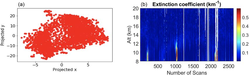
392                                                            G. Farhani et al.: Machine learning for lidar data classification

   In this article we propose both supervised and unsuper-           for the lidar data classification. Furthermore, the algorithms
vised machine learning approaches for level-0 lidar data clas-       which are used in the paper are explained in detail. In Sect. 3
sification and clustering. ML techniques hold great promise          we show classification and clustering results for the PCL sys-
for application to the large data sets obtained by the cur-          tem. In Sect. 4, a summary of the ML approach is provided,
rent and future generation of high temporal–spatial resolu-          and the future directions are discussed.
tion lidars. ML has been recently used to distinguish between
aerosols and clouds for the Cloud-Aerosol Lidar and Infrared
Pathfinder Satellite Observations (CALIPSO) level-2 mea-             2     Machine learning algorithms
surements (Zeng et al., 2019). Furthermore, Nicolae et al.
                                                                     2.1    Instrument description and machine learning
(2018) used a neural network algorithm to estimate the most
                                                                            classification of data
probable aerosol types in a set of data obtained from the Eu-
ropean Aerosol Research Lidar Network (EARLINET). Both               The PCL is a Rayleigh–Raman lidar which has been opera-
Zeng et al. (2019) and Nicolae et al. (2018) concluded that          tional since 1992. Details about PCL instrumentation can be
their proposed ML algorithms can classify large sets of data         found in Sica et al. (1995). From 1992 to 2010, the lidar was
and can successfully distinguish between different types of          located at the Delaware Observatory (42.5◦ N, 81.2◦ W) near
aerosols.                                                            London, Ontario, Canada. In 2012, the lidar was moved to
   A common way of classifying profiles is to define a thresh-       the Environmental Science Western Field Station (43.1◦ N,
old for the signal-to-noise ratio at some altitude: any scan that    81.3◦ W). The PCL uses a second harmonic of an Nd:YAG
does not meet the pre-defined threshold value is flagged as          solid state laser. The laser operates at 532 nm and has a repe-
bad. In this method, bad profiles may be incorrectly flagged         tition rate of 30 Hz at 1000 mJ. The receiver is a liquid mer-
as good, as they might pass the threshold criteria but have          cury mirror with the diameter of 2.6 m. The PCL currently
the wrong shape at other altitudes. Recently, Wing et al.            has four detection channels:
(2018) suggested that a Mann–Whitney–Wilcoxon rank-sum
metric could be used to identify bad profiles. In the Mann–              1. A high-gain Rayleigh (HR) channel that detects the
Whitney–Wilcoxon test, the null hypothesis that the two pop-                back-scattered counts from 25 to 110 km altitude (verti-
ulations are the same is tested against the alternate hypothesis            cal resolution: 7 m).
that there is a significant difference between the two popula-
tions. The main advantage of this method is that it can be               2. A low-gain Rayleigh (LR) channel that detects the back-
used when the data distribution does not follow a Gaussian                  scattered counts from 25 to 110 km altitude (this chan-
distribution. However, Monte Carlo simulations have shown                   nel is optimized to detect counts at lower altitudes where
that when the two populations have similar medians, but dif-                the high-intensity back-scattered counts can saturate the
ferent variances, the Mann–Whitney–Wilcoxon can wrong-                      detector and cause non-linearity in the observed signal;
fully accept the alternative hypothesis (Robert and Casella,                thus, using the low-gain channel, at lower altitudes, the
2004). Here, we propose a machine learning (ML) approach                    signal remains linear) (vertical resolution: 7 m).
for level-0 data classification. The classification of lidar pro-        3. A nitrogen Raman channel that detects the vibrational
files is based on supervised ML techniques which will be                    Raman-shifted back-scattered counts above 0.5 km in
discussed in detail in Sect. 2.                                             altitude (vertical resolution: 7 m).
   Using an unsupervised ML approach, we also examined
the capability of ML to detect anomalies (traces of wildfire             4. A water vapour Raman channel that detects the vi-
smoke in lower stratosphere). The PCL is capable of detect-                 brational Raman-shifted back-scattered counts above
ing the smoke injected into the lower stratosphere from wild-               0.5 km in altitude (vertical resolution: 24 m).
fires (Doucet, 2009; Fromm et al., 2010). We are interested
in whether the PCL can automatically (by using ML meth-              The Rayleigh channels are used for atmospheric temperature
ods) detect aerosol loads in the upper troposphere and lower         retrievals, and the water vapour and nitrogen channels are
stratosphere (UTLS) after major wildfires. Aerosols in the           used to retrieve water vapour mixing ratio.
UTLS and stratosphere have important impacts on the ra-                 In our lidar scan classification using supervised learning,
diative budget of the atmosphere. Recently, Christian et al.         we have a training set in which, for each scan, counts at
(2019) proposed that smoke aerosols from the forest fires,           each altitude are considered as an attribute, and the classi-
unlike the aerosols from the volcanic eruptions, can have a          fication of the scan is the output value. Formally, we are
net positive radiative forcing. Considering that the number of       trying to learn a prediction function f (x): x → y, which
forest fires have increased, detecting the aerosol loads from        minimizes the expectation of some loss function L(y, f ) =
                                                                                    predicted
fires in the UTLS and accounting for them in atmospheric             6iN (yitrue − yi         ), where yitrue is the actual value (label)
                                                                                                                      predicted
and climate models is important.                                     of the classification for each data point; yi              is the pre-
   Section 2 is a brief description of the characteristics of the    diction generated from the prediction function, and N is the
lidars we used and an explanation of how ML can be useful            length of the data set (Bishop, 2006). Thus, the training set is

Atmos. Meas. Tech., 14, 391–402, 2021                                                    https://doi.org/10.5194/amt-14-391-2021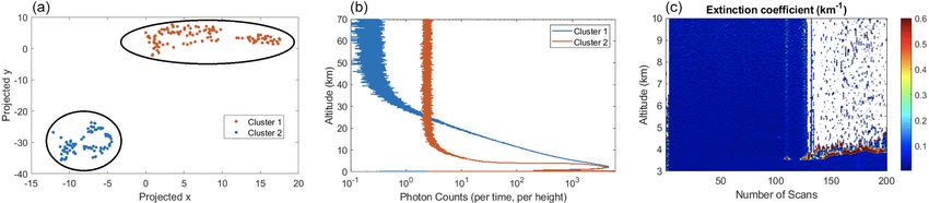
G. Farhani et al.: Machine learning for lidar data classification                                                                    393

Figure 1. Example of measurements taken by PCL Rayleigh and Raman channels. (a) Examples of bad profiles for both Rayleigh and Raman
channels. In this plot, the signals in cyan and dark red have extremely low laser power, the purple signal has extremely high background
counts, and the signal in orange has a distorted shape and high background counts. (b) Example of a good scan in the Rayleigh channel. (c)
Example of cloudy sky in the nitrogen (Raman) channel. At about 8 km a layer of either cloud or aerosol occurs.

a matrix with size (m, n), and each row of the matrix presents         decided to use the classical machine learning algorithms as
a lidar scan in the training set. The columns of this matrix           they can provide a better explanation of feature selection.
(except the last column) are photon counts at each altitude.
The last column of the matrix shows the classifications of             2.2   Support vector machine algorithms
each scan. Examples of each scan’s class for PCL measure-
ments using Rayleigh and nitrogen Raman digital channels
                                                                       SVM algorithms are popular in the remote sensing commu-
are shown in Fig. 1.
                                                                       nity because they can be trained with relatively small data
   We also examined unsupervised learning to generate
                                                                       sets, while producing highly accurate predictions (Mantero
meaningful clusters. We are interested in determining
                                                                       et al., 2005; Foody and Mathur, 2004). Moreover, unlike
whether the lidar profiles, based on their similarities (sim-
                                                                       some statistical methods such as the maximum likelihood
ilar features), will be clustered together. For our clustering
                                                                       estimation that assume the data are normally distributed,
task, a good ML method will distinguish between high back-
                                                                       SVM algorithms do not require this assumption. This prop-
ground counts, low-laser power profiles, clouds, and high-
                                                                       erty makes them suitable for data sets with unknown distri-
laser profiles, and put each of these in a different cluster.
                                                                       butions. Here, we briefly describe how SVM works. More
Moreover, using unsupervised learning, anomalies in profiles
                                                                       details on the topic can be found in Burges (1998) and Vap-
(a.k.a. traces of smoke in higher altitudes) should be appar-
                                                                       nik (2013).
ent.
                                                                          The SVM algorithm finds an optimal hyperplane that sep-
   Many algorithms have been developed for both supervised
                                                                       arates the data set into a distinct predefined number of classes
and unsupervised learning. In the following section, we intro-
                                                                       (Bishop, 2006). For binary classification in a linearly separa-
duce support vector machine (SVM), decision tree, random
                                                                       ble data set, a target class yi ∈ {1, −1} is considered with a
forest, and gradient boosting tree methods as part of ML al-
                                                                       set of input data vectors x i . The optimal solution is obtained
gorithms that we have tested for sorting lidar profiles. We
                                                                       by maximizing the margin (w) between the separating hyper-
also describe the t-distributed stochastic neighbour embed-
                                                                       plane and the data. It can be shown that the optimal hyper-
ding method and density-based spatial clustering as unsuper-
                                                                       plane is the solution of the constrained quadratic equation:
vised algorithms which were used in this study.
   Recently, deep neural networks (DNNs) have received at-
tention in the scientific community. In the neural network                         1
approach the loss function computes the error between the              minimize: kwk2 ,                                               (1)
                                                                                   2
output scores and target values. The internal parameters               constraint: yi (w| x i + b)>1.                                 (2)
(weights) in the algorithm are modified such that the error
becomes smaller. The process of tuning the weights contin-
ues until the error is not decreasing anymore. A typical deep          In the above equation the constraint is a linear model where
learning algorithm can have hundreds of millions of weights,           w and the intercept (b) are unknowns (need to be optimized).
inputs and target values. Thus, the algorithm is useful when           To solve this constrained optimization problem, the Lagrange
dealing with large sets of images and text data. Although              function can be built:
DNNs are power full tools, they are acting as black boxes
and important questions such as what features in the input                            1      X
                                                                                        w2 −   αi yi (w | x i + b) − 1 ,

data are more important remain unknown. For this study we              L(w, b, α) =                                                   (3)
                                                                                      2      i

https://doi.org/10.5194/amt-14-391-2021                                                      Atmos. Meas. Tech., 14, 391–402, 2021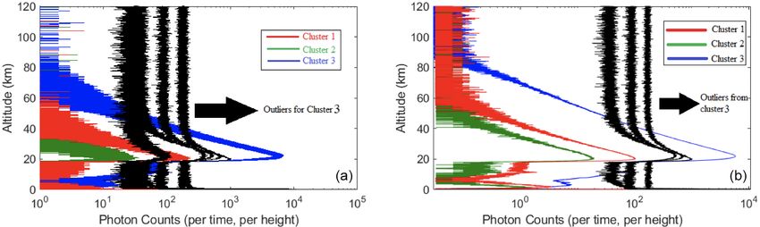
394                                                            G. Farhani et al.: Machine learning for lidar data classification

where αi are Lagrangian multipliers. Setting the derivatives           – Evaluating the splits. Using a score measure, at each
of L(w, b, α) with respect to w and b to zero:                           node, we can decide what the best question is to be
     X                                                                   asked and what the best feature is to be used. As the
w=      αi y i x i ,                                     (4)             goal of splitting is to find the purest learning subset that
        i
X                                                                        is in each leaf, we want the output labels to be the same;
 αi yi = 0.                                                  (5)         called purifying. Shannon entropy (see below) is used to
 i                                                                       evaluate the purity of each subgroup. Thus, a split that
Thus we can rewrite the Lagrangian as follows:                           reduces the entropy from one node to its descendent is
                                                                         favourable.
                X            1 XX                |
L(w, b, α) =          αi −         αi αj yi yj x i x j .     (6)
                             2 i j                                     – Deciding to stop splitting. We set rules to define when
                  i
                                                                         the splitting should be stopped, and a node becomes a
It is clear that the optimization process only depends on the            leaf. This decision can be data-driven. For example, we
dot product of the samples.                                              can stop splitting when all objects in a node have the
   Many real-world problems involve non-linear data sets in              same label (pure node). The decision can be defined by
which the above methodology will fail. To tackle the non-                a user as well. For example, we can limit the maximum
linearity, using a non-linear function 8(x) the feature space            depth of the tree (length of the path between root and a
is mapped into higher-dimensional feature space. The La-                 leaf).
grangian function can be re-written as follows:
                                                                        In a decision tree, by performing a full scan of attribute
             X      1 XX                                             space the optimal split (at each local node) is selected, and
L(w, b, α) =   αi −       αi αj yi yj k(x i , x j ),         (7)
             i
                    2 i j                                            irrelevant attributes are discarded. This method allows us to
                                                                     identify the attributes that are most important in our decision-
k(x i , x j ) = 8(x i )| 8(x j ),                            (8)     making process.
where k(x i , x j ) is known as the kernel function. Kernel func-       The metric used to judge the quality of the tree splitting
tions let the feature space be mapped into higher-dimensional        is Shannon entropy (Shannon, 1948). Shannon entropy de-
space without the need to calculate the transformation func-         scribes the amount of information gained with each event and
tion (only the kernel is needed). More details on SVM and            is calculated as follows:
kernel functions can be found in Bishop (2006).
                                                                     H (x) = −6pi log pi ,                                            (9)
   To use SVM as a multi-class classifier, some adjustments
need to be made to the simple SVM binary model. Meth-
                                                                     where pi represents a set of probabilities that adds up to 1.
ods like a directed acyclic graph, one-against-all, and one-
                                                                     H (x) = 0 means that no new information was gained in the
against-others are among the most successful techniques for
                                                                     process of splitting, and H (x) = 1 means that the maximum
multi-class classification. Details about these methods can be
                                                                     amount of information was achieved. Ideally, the produced
found in Knerr et al. (1990).
                                                                     leaves will be pure and have low entropy (meaning all of the
2.3     Decision trees algorithms                                    objects in the leaf are the same).

Decision trees are nonparametric algorithms that allow com-          2.4   Random forests
plex relations between inputs and outputs to be modelled.
                                                                     The random forest (RF) method is based on “growing” an
Moreover, they are the foundation of both random forest and
                                                                     ensemble of decision trees that vote for the most popular
boosting methods. A comprehensive introduction to the topic
                                                                     class. Typically the bagging (bootstrap aggregating) method
can be found in Quinlan (1986). Here, we briefly describe
                                                                     is used to generate the ensemble of trees (Breiman, 2002).
how a decision tree is built.
                                                                     In bagging, to grow the kth tree, a random vector θ k from
   A decision tree is a set of (binary) decisions represented
                                                                     the training set is selected. The θ k vector is independent of
by an acyclic graph directed outward from a root node to
                                                                     the past vectors (θ 1 , . . ., θ k−1 ) but has the same distribution.
each leaf. Each node has one parent (except the root) and can
                                                                     Then, by selecting random features, the kth tree is generated.
have two children. A node with no children is called a leaf.
                                                                     Each tree is a classifier (h(θ k , x)) that casts a vote. During
Decision trees can be complex depending on the data set. A
                                                                     the construction of decision trees, in each interior node, the
tree can be simplified by pruning, which means leaves from
                                                                     Gini index is used to evaluate the subset of selected features.
the upper parts of the trees will be cut. To grow a decision
                                                                     The Gini index is the measure of impurity of data (Lerman
tree, the following steps are taken.
                                                                     and Yitzhaki, 1984; Liaw et al., 2002). Thus, it is desirable to
     – Defining a set of candidate splits. We should answer a        select a feature that results in a greater decrease in the Gini
       question about the value of a selected input feature to       index (partitioning the data into distinct classes). For a split
       split the data set into two groups.                           at node n the index can be calculated as 1 − 6i=1     2 P 2 , where
                                                                                                                                i

Atmos. Meas. Tech., 14, 391–402, 2021                                                    https://doi.org/10.5194/amt-14-391-2021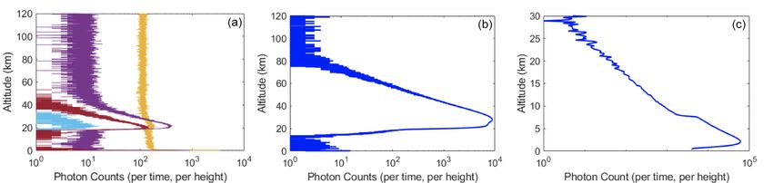
G. Farhani et al.: Machine learning for lidar data classification                                                              395

Pi is the frequency of class i in the node n. Finally, the class   2.6   The t-distributed stochastic neighbour embedding
label is determined via majority voting among all the trees              method
(Liaw et al., 2002).
   One major problem in ML is that when the algorithm be-          A detailed description of unsupervised learning can be found
comes too complicated and perfectly fits the training data         in Hastie et al. (2009). Here, we briefly introduce two of the
points, it loses its generality and performs poorly on the test-   unsupervised algorithms that are used in this paper. The t-
ing set. This problem is known as overfitting. For RF, in-         distributed stochastic embedding (t-SNE) method is an unsu-
creasing the number of trees can help with the overfitting         pervised ML algorithm that is based on stochastic neighbour
problem. Other parameters that can significantly influence         embedding (SNE). In the SNE, the data points are placed
RFs are the tree depth and the number of trees. As a tree          into a low-dimensional space such that the neighbourhood
gets deeper it has more splits while growing more trees in a       identity of each data point is preserved (Hinton and Roweis,
forest yields a smaller prediction error. Finding the optimal      2002). The SNE is based on finding the probability that data
depth of each tree is a critical parameter. While leaves in a      point i has data point j as its neighbour, which can formally
short tree may contain heterogeneous data (the leaves are not      be written as follows:
pure), tall trees can suffer from poor generalization (overfit-                      2 )
                                                                               exp(−di,j
ting problem). Thus, the optimal depth provides a tree with        Pi,j = P               2
                                                                                                  ,                           (10)
pure leaves and great generalization. Detailed discussion on                   k6=i exp(−di,k )
the RFs can be found in Liaw et al. (2002).                        where Pi,j is the probability of i selecting j as its neighbour
                                                                         2 is the squared Euclidean distance between two points
                                                                   and di,j
2.5   Gradient boosting tree methods
                                                                   in the high dimensional space. This can be written as follows:
Boosting methods are based on the idea that combining many                  k(xi − xj )k2
                                                                    2
“weak” approximation models (a learning algorithm that is          di,j =                   ,                                 (11)
                                                                                2σi2
slightly more accurate than 50 %) will eventually boost the
predictive performance (Knerr et al., 1990; Schapire, 1990).       where σi is defined so that the entropy of the distribution
Thus, many “local rules” are combined to produce highly ac-        becomes log κ, and κ is the “perplexity”, which is set by the
curate models.                                                     user and determines how many neighbours will be around a
   In the gradient boosting method, simple parametrized            selected point.
models (base models) are sequentially fitted to current resid-        The SNE tries to model each data point, xi , at the higher
uals (known as pseudo-residuals) at each iteration. The resid-     dimension, by a point yi at a lower dimension such that the
uals are the gradients of the loss function (they show the dif-    similarities in Pi,j are conserved. In this low-dimensional
ference between the predicted value and the true value) that       map, we assume that the points follow a Gaussian distribu-
we are trying to minimize. The gradient boosting tree (GBT)        tion. Thus, the SNE tries to make the best match between the
algorithm is a sequence of simple trees generated such that        original distribution (pi,j ) and the induced probability dis-
each successive tree is grown based on the prediction resid-       tribution (qi,j ). This match is determined by minimizing the
ual of the preceding tree with the goal of reducing the new        error between the two distributions, and the best match is de-
residual. This “additive weighted expansion” of trees will         veloped. The induced probability is defined as follows:
eventually become a strong classifier (Knerr et al., 1990).
This method can be successfully used even when the rela-                      exp(−k(yi − yj )k2 )
                                                                   qi,j = P                         2
                                                                                                       .                      (12)
tion between the instances and output values are complex.                     k6=i exp(−k(yi − yk )k )
Compared to the RF model, which is based on building many
                                                                      The SNE algorithm aims to find a low-dimensional data
independent models and combining them (using some aver-
                                                                   representation such that the mismatch between pi,j and qi,j
aging techniques), the gradient boosting method is based on
                                                                   become minimized; thus in the SNE the Kullback–Leibler
building sequential models.
                                                                   divergences is defined as the cost function. Using the gradi-
   Although the GBTs show overall high performance, they
                                                                   ent descent method the cost function is minimized. The cost
require large set of training data and the method is quite sus-
                                                                   function is written as follows:
ceptible to noise. Thus, for smaller training data set the algo-
rithm suffers from overfitting. As the size of our data set is                                             pj |i
                                                                   cost = 6i KL(Pi kQi ) = 6i 6j pj |i log        ,         (13)
large, GBT could potentially be a reliable algorithm for the                                               qj ||i
classification of lidar profiles in this case.                     where Pi is the conditional probability distribution of all data
                                                                   points given data points xi , and Qi is the conditional proba-
                                                                   bility for all the data points given data points yi .
                                                                      The t-SNE uses a similar approach but assumes a lower-
                                                                   dimensional space, which instead of being a Gaussian distri-
                                                                   bution follows Student’s t distribution with a single degree

https://doi.org/10.5194/amt-14-391-2021                                                     Atmos. Meas. Tech., 14, 391–402, 2021
396 G. Farhani et al.: Machine learning for lidar data classification
– Core point. Point A is a core point if within the distance
of at least minPts points (including A) exist.
– Reachable point. Point B is reachable from point A if
there is a path (P1 , P2 , . . ., Pn ) from A to B (P1 = A).
All points in the path, with the possible exception of
point B, are core points.
– Outlier point. Point C is an outlier if it is not reachable
from any point.
In this method, an arbitrary point (that has not been vis-
ited before) is selected, and using the above steps the neigh-
bour points are retrieved. If the created cluster has a sufficient
number of points (larger than minPts) a cluster is started. One
advantage of DBSCAN is that the method can automatically
Figure 2. Red curve: the Gaussian distribution for data points, ex- estimate the numbers of clusters.
tending from −5σ to 5σ . The mean of the distribution is at 0. Blue
curve: the Student’s t distribution over the same range. The distri- 2.8 Hyper-parameter tuning
bution is heavy-tailed, compared to the Gaussian distribution.
Machine learning methods are generally parametrized by a
set of hyper-parameters, λ. An optimal set λbest will result
of freedom. Thus, since a heavy-tailed distribution is used to in an optimal algorithm which minimizes the loss function.
measure similarities between the points in the lower dimen- This set can be formally written as follows:
sion, the data points that are less similar will be located fur-
ther from each other. To demonstrate the difference between λbest = argmin{L(Xtest ; A(Xtrain , λ))}, (15)
the Student’s t distribution and the Gaussian distribution, we
plot the two distributions in Fig. 2. Here, the x values are where A is the algorithm and Xtest and Xtrain are test
within 5σ and −5σ . The Gaussian distribution with the mean and training data. Searching to find the best set of hyper-
at 0 and the Student’s t distribution with the degree of free- parameters is mostly done using grid search method in which
dom of 1 are generated. As is shown in the figure, the t dis- a set of values on a predefined grid is proposed. Implement-
tribution peaks at a lower value and has a more pronounced ing each of the proposed hyper-parameters, the algorithm
tail. The above approach gives t-SNE an excellent capability will be trained, and the prediction results will be compared.
for visualizing data, and thus, we use this method to allow Most algorithms have only a few hyper-parameters. Depend-
scan classification via unsupervised learning. More details on ing on the learning algorithm, the size of training, and test
SNE and t-SNE can be found in Hinton and Roweis (2002) data sets, the grid search can be a time-consuming approach.
and Maaten and Hinton (2008). Thus automatic hyper-parameter optimization has gained in-
terest; details on the topic can be found in Feurer and Hutter
2.7 Density-based spatial clustering of applications (2019).
with noise (DBSCAN)
3 Result for supervised and unsupervised learning
DBSCAN is an unsupervised learning method that relies on
using the PCL system
density-based clustering and is capable of discovering any ar-
bitrary shape from a collection of points. There are two input
3.1 Supervised ML results
parameters to be set by the user: minPts, which indicates the
minimum number of points needed to make a cluster, and To apply supervised learning to the PCL system, we ran-
such that the neighbourhood of point p denoting as N (p) domly chose 4500 profiles from the LR, HR, and the nitro-
is defined as follows: gen vibrational Raman channels. These measurements were
taken on different nights in different years and represent
N (p) = {q ∈ D | dis(p, q) ≤ }, (14) different atmospheric conditions. For the LR and HR dig-
ital Rayleigh channels, the profiles were labelled as “bad
where p and q are two points in data set (D) and dist(p, q) profiles” and “good profiles”. For the nitrogen channel we
represents any distance function. Defining the two input pa- added one more label that represents profiles with traces of
rameters, we can make clusters. In the clustering process data clouds or aerosol layers, called “cloudy” profiles. Here, by
points are classified into three groups: core points, (density) “cloud” we mean a substantial increase in scattering relative
reachable points, and outliers, defined as follows. to a clean atmosphere, which could be caused by clouds or
Atmos. Meas. Tech., 14, 391–402, 2021 https://doi.org/10.5194/amt-14-391-2021G. Farhani et al.: Machine learning for lidar data classification 397
Table 1. Accuracy scores for the training and the test set for SVM, Table 2. Precision and recall values for the nitrogen, LR, and HR
RF, and GBT models. Results are shown for HR, LR, and nitrogen channels. The precision and recall values are calculated using the
channels. GBT model.
Test set Nitrogen channel
Channel SVM RF GBT Scan type Precision Recall
HR 83 % 97 % 98 % Cloud 0.94 0.91
LR 88 % 97 % 97 % Clear 0.96 0.98
Nitrogen 88 % 95 % 96 % Bad 1.00 1.00
Training set LR channel
Channel SVM RF GBT Scan type Precision Recall
HR 90 % 98 % 99 % Clear 0.99 0.99
LR 90 % 98 % 98 % Bad 0.96 0.95
Nitrogen 88 % 94 % 95 %
HR channel
Scan type Precision Recall
aerosol layers. The HR and LR channels are seldom affected Clear 0.98 1.00
by clouds or aerosols as the chopper is not fully open until Bad 0.98 0.94
about 20 km. Furthermore, labelling the water vapour chan-
nel was not attempted for this study, due to its high natural
variability in addition to instrumental variability. gorithm can distinguish between good and bad profiles. The
We used 70 % of our data for the training phase and we precision and recall are defined as follows:
kept 30 % of data for the test phase (meaning that during
the training phase 30 % of data stayed isolated and the al- true positive
precision = ,
gorithm was built without considering features of the test true positive + false positive
data). In order to overcome the overfitting issue we used the true positive
recall = . (16)
k-fold cross-validation technique, in which the data set is di- true positive + false negative
vided into k equal subsets. In this work we used 5-fold cross-
validation. The accuracy score is the ratio of correct predic- The precision and recall for the nitrogen channel for each
tions to the total number of predictions. We used accuracy as category (clear, cloud, and bad) are shown in Table 2 as well.
a metric of evaluating the performance of the algorithms. We The GBT and RF algorithms, both have high accuracy results
used the Python scikit-learn package to train our ML mod- on HR and LR channels. The accuracy of the model on the
els. The prediction scores resulting from the cross-validation training set on the LR channel for both RF and GBT are 99 %
method as well as from fitting the models on the test data set and on the test set are 98 %. The precision and recall values
is shown in Table 1. for the clear profiles are close to unity and for the bad profiles
We also used the confusion matrix for further evaluations they are 0.95 and 0.96 respectively. The HR channel also has
where the good profiles are considered as “positive” and the a high accuracy of 99 % in the training set for both RF and
bad profiles are considered as “negative”. A confusion matrix GBT, and the accuracy score in the testing set is 98 %. The
can provide us with the number of the following: precision and recall values in Table 2 are also similar to the
LR channel.
– True positives (TP) – the number of profiles that are cor- For the nitrogen channel the GBT algorithm has the high-
rectly labelled as positive (clean profiles); est accuracy of 95 %, while the RF algorithm has accuracy
of 94 %. The confusion matrix of the test result for the GBT
– False positives (FP) – the number of profiles that are algorithm (the one with the highest accuracy) is shown in
incorrectly labelled as positive; Fig. 3a. The algorithm can perform almost perfectly on dis-
– True negatives (TN) – the number of profiles that are tinguishing bad profiles (only one bad scan was wrongly la-
correctly labelled as negative (bad profiles); belled as cloudy). The cloud and clear profiles for most pro-
files are labelled correctly; however, for a few profiles the
– False negatives (FN) – the number of profiles that are model mislabelled clouds as clear profiles.
incorrectly labelled as negative.
3.2 Unsupervised ML results
A perfect algorithm will result in a confusion matrix in
which FP and FN are zeros. Moreover, the precision and re- The t-SNE algorithm clusters the measurements by means
call can be employed to give us an insight into how our al- of pairwise similarity. The clustering can differ from night
https://doi.org/10.5194/amt-14-391-2021 Atmos. Meas. Tech., 14, 391–402, 2021398 G. Farhani et al.: Machine learning for lidar data classification
Figure 3. The confusion matrices for nitrogen channel (a), LR channel (b), and HR channel (c). In a perfect model, the off-diagonal elements
of the confusion matrix are zeros.
to night due to atmospheric and systematic variability. On
nights where most profiles are similar, fewer clusters are
seen, and on other nights when the atmospheric or the instru-
ment conditions are more variable, more clusters are gener-
ated. The t-SNE makes clusters but does not estimate how
many clusters are built, and the user must then estimate the
number of clusters. To automate this procedure, after apply-
ing the t-SNE to lidar measurements we use the DBSCAN
algorithm to estimate the number of clusters. The second step
of applying DBSCAN is used to estimate the number of gen-
erated clusters by t-SNE.
To demonstrate how clustering works, we show measure-
ments from the PCL LR channel and the nitrogen channels.
Here, we use the t-SNE on 15 May 2012 that contains both
bad and good profiles. We also show the clustering result for Figure 4. Clustering of lidar return signal type using the t-SNE al-
gorithm for 339 profiles from the low-gain Rayleigh measurement
the nitrogen channel on 26 May 2012. We chose this night
channel on the night of 15 May 2012. The profiles are automati-
because at the beginning of the measurements the sky was cally clustered into three different groups selected by the algorithm.
clear but the sky became cloudy. Cluster 3 has some outliers.
On the night of 15 May 2012, the t-SNE algorithm gen-
erates three distinct clusters for the LR channel (Fig. 4).
These clusters correspond to different types of lidar return files. The result of clustering is shown in Fig. 6a in which two
profiles. Figure 5a shows all the signals for each of the clus- well-distinguished clusters are generated, where one cluster
ters. The maximum number of photon counts and the value represents the cloudy and the other represents the non-cloudy
and the height of the background counts are the identifiers be- profiles. The averaged signal for each cluster is plotted in
tween different clusters. Thus, cluster 3 with low background Fig. 6b. Moreover, the particle extinction profile at altitudes
counts and high maximum counts represents a group of pro- between 3 and 10 km is plotted in the same figure (Doucet,
files which are labelled as good profiles in our supervised 2009). The first 130 profiles are clean and the last 70 pro-
algorithms. Cluster 1 represents the profiles with lower than files are severely affected by thick clouds; thus the extinction
normal laser powers, and cluster 2 shows profiles with ex- profile is consistent with our t-SNE classification result.
tremely low laser powers. To better understand the difference The t-SNE method can be used as a visualization tool;
between these clusters, Fig. 5b shows the average signal. Fur- however, to evaluate each cluster the user either needs to ex-
thermore, the outliers of cluster 3 (shown in black) identify amine profiles within each cluster or use one of the aforemen-
the profiles with extremely high background counts. This re- tioned classification methods. For example Fig. 4 shows this
sult is consistent with our supervised method, in which we night of measurement had some major differences among the
had good profiles (cluster 3), and bad profiles which are pro- collected profiles (if all the profiles were similar only one
files with lower laser power (clusters 1 and 2). cluster would be generated). But, to evaluate the cluster the
Using the t-SNE, we also have clustered profiles for the profiles within each cluster must be examined by a human,
nitrogen channel with the measurements taken on 26 May or a supervised ML should be used to label each cluster.
2012. This night was selected because the sky conditions
changed from clear to cloudy. The measurements from this 3.3 PCL fire detection using the t-SNE algorithm
night allows us to test our algorithm and determine how well
it can distinguish cloudy profiles from the non-cloudy pro- The t-SNE can be used for anomaly detection. As fire’s
smoke in the stratosphere is a relatively rare event, we can
Atmos. Meas. Tech., 14, 391–402, 2021 https://doi.org/10.5194/amt-14-391-2021G. Farhani et al.: Machine learning for lidar data classification 399 Figure 5. (a) All 339 profiles collected by the PCL system LR channel on the night of 15 May 2012. The sharp cutoff for all profiles below 20 km is due to the system’s mechanical chopper. The green signals have extremely low power. The red line represents all signals with low return signal and the blue line indicates the signals that are considered good profiles. The black lines are signals with extremely high backgrounds. (b) Each line represents an average of the signals within a cluster. The red line is the average signal for profiles with lower laser power (cluster 1). The green line is the average signal for profiles with really low laser power (cluster 2). The blue line is the average signal for profiles with strong laser power (cluster 3). The black line indicates the outliers that have extremely high background counts and are outliers belonging to cluster 3 (blue curve). The background counts in the green line start at about 50 km, whereas for the red line the background starts at almost 70 km and for the blue line profiles the background starts at 90 km. Figure 6. (a) Profiles for the nitrogen channel on the night of 15 May 2012 were clustered into two different groups using the t-SNE algorithm. (b) The red line (cluster 2) is the average of all signals within this cluster and indicates the profiles in which clouds are detectable. The blue line (cluster 2) is the average of all signals within this cluster and indicates the clear profiles (non-cloudy condition). (c) The particle extinction profile for the night shows the last 70 profiles are affected by thick clouds at about 4.5 km altitude. test the algorithms to identify these events. Here, we used the is generated), as the lidar measurement were affected by the t-SNE to explore traces of aerosol in stratosphere within one wildfire in Saskatchewan, and nights of measurements in July month of measurements. We expect that the t-SNE would 2007 are used as an example of nights with no high loads of generate a single cluster for a month with no trace of strato- aerosol in stratosphere (only one cluster is generated). spheric aerosols that means no “anomalies” have been de- The wildfires in Saskatchewan during late June and early tected. The algorithm should generate more than one clus- July 2002 produced a massive amount smoke that was trans- ter in the case of detecting stratospheric aerosols. We use ported southward. As the smoke from the fire can reach to the DBSCAN algorithm to automatically estimate the num- higher altitudes (reaching to lower stratosphere), we are in- ber of generated profiles. In DBSCAN, most of the bad pro- terested in seeing whether we can automatically detect strato- files will be tagged as noise (meaning that they do not belong spheric aerosol layers during wildfire events. The PCL was to any cluster). Here we are showing two examples, in one operational on the nights of 8, 9, 10, 19, 21, 29, and 30 June of which the stratospheric smoke exists and our algorithm 2002. During these nights, 1961 lidar profiles were collected generates more than one cluster. In the other example strato- in the nitrogen channel. We used the t-SNE algorithm to ex- spheric smoke is not present in the profiles, and the algo- amine if the algorithm can detect and cluster the profiles with rithm only generates one cluster. The nightly measurements the trace of wildfire in higher altitudes, using profiles in the of June 2002 are used as an example of a month in which altitude range of 8 to 25 km. To automatically estimate the the t-SNE can detect anomalies (thus more than one cluster number of produced clusters we used the DBSCAN algo- https://doi.org/10.5194/amt-14-391-2021 Atmos. Meas. Tech., 14, 391–402, 2021
400 G. Farhani et al.: Machine learning for lidar data classification
are more confident in claiming that the detected aerosol lay-
ers are traces of smoke, as shown in Fromm et al., 2010).
4 Summary and conclusion
We introduced a machine learning method to classify raw
lidar (level-0) measurements. We used different ML meth-
ods on elastic and inelastic measurements from the PCL li-
dar systems. The ML methods we used and our results are
summarized as follows.
1. We tested different supervised ML algorithms, among
which the RF and the GBT performed better, with a suc-
cess rate above 90 % for the PCL system.
Figure 7. Profiles for the nitrogen channel for the nights of June
2002 were clustered into four different groups using the t-SNE al- 2. The t-SNE unsupervised algorithm can successfully
gorithm. The small cluster in cyan indicates the group of profiles cluster profiles on nights with both consistent and vary-
that do not belong to any of the other clusters in the DBSCAN al- ing lidar profiles due to both atmospheric conditions and
gorithm. system alignment and performance. For example, if dur-
ing the measurements the laser power dropped or clouds
became present, the t-SNE showed different clusters
representing these conditions.
rithm. We set the minPts condition to 30, and the value to 3. 3. Unlike the traditional method of defining a fixed thresh-
The DBSCAN algorithm estimated four clusters and few pro- old for the background counts, in supervised ML ap-
files remained as the noise, which do not belong to any other proach the machine can distinguish high background
clusters (shown in cyan, in Fig. 7). To investigate whether counts by looking at the labels of the training set. In
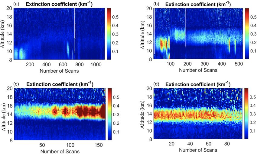
profiles with layers are clustered together the particle extinc- the unsupervised ML approach, by looking at the sim-
tion profile for each generated cluster is plotted (Fig. 8). Most ilarities between the two profiles and defining a dis-
of the profiles in cluster 1 are clean and no sign of particles tance scale, good profiles will be grouped together. High
can be seen in these profiles (Fig. 8a), cluster 2 contains all background counts can be grouped in a smaller group.
profiles with mostly small traces of aerosol between 10 and Most of the time the number of bad profiles are small;
14 km (Fig. 8b). The presence of high loads of aerosol can thus they will be labelled as noise.
clearly detected in the particle extinction profiles for both
cluster 3 and 4; the difference between the two clusters is We successfully implemented supervised and unsuper-
in the height at which the presence of aerosol layer is more vised ML algorithms to classify lidar measurement profiles.
distinguished (Fig. 8d and c). Profiles in the last two clusters The ML is a robust method with high accuracy that enables
belong to the last two nights of measurements on June 2002 us to precisely classify thousands of lidar profiles within a
which are coincidental with the smoke being transported to short period of time. Thus, with accuracy of higher than 95 %
London from the wildfire in Saskatchewan. this method has a significant advantage over previous meth-
We also examined a total of 2637 profiles in the altitude ods of classifying. For example, in the supervised ML, we
range of 8 to 25 km obtained from 10 nights of measurements train the machine by showing (labelling) different profiles
in July 2007. As we expected, no anomalies were detected in different conditions. When the machine has seen enough
(Fig. 9). The particle extinction profile of July 2007 also in- examples of each class (which is a small fraction of the en-
dicates that at the altitude range of 8 to 25 km no aerosol load tire database), it can classify the un-labelled profiles with no
exists (Fig. 9). need to pre-define any condition for the system. Furthermore,
Thus, using the t-SNE method we can detect anomalies in in the unsupervised learning method, no labelling is needed,
the UTLS. In the UTLS region, for the clear atmosphere we and the whole classification is free from subjective biases of
expect to see a single cluster, and when aerosol loads exist the individual marking the profiles (which is important for
at least two clusters will be generated. We are implementing large atmospheric data sets ranging over decades). Using ML
the t-SNE on one month of measurements, and when the al- avoids the problem of different observers classifying profiles
gorithm generates more than one cluster we examine profiles differently. We also showed that the unsupervised schema
within that cluster. However, at the moment, because we only has the potential to be used as an anomaly detector, which
use the Raman channel it is not possible for us to distinguish can alert us when there is a trace of aerosol in the UTLS re-
between smoke traces and cirrus clouds (unless the trace is gion. We are planning to expand our unsupervised learning
detected in altitudes above 14 km, similar to Fig. 8 where we method to both Rayleigh and nitrogen channels to be able to
Atmos. Meas. Tech., 14, 391–402, 2021 https://doi.org/10.5194/amt-14-391-2021G. Farhani et al.: Machine learning for lidar data classification 401
Figure 8. The t-SNE generates four clusters for profiles of nitrogen channels in July 2007. (a) Most of the profiles are clean and no sign of
particles can be seen. (b) Profiles with mostly small traces of aerosol between 10 and 14 km. (c, d) The presence of high loads of aerosol can
clearly be detected.
Figure 9. (a) The particle extinction profile of July 2007 indicates no significant trace of stratospheric aerosols. (b) The t-SNE generates a
single cluster for all of 2637 profiles of nitrogen channel for July 2007.
correctly identify and distinguish cirrus clouds from smoke DataLink button or via FTP at http://ftp.cpc.ncep.noaa.gov/ndacc/
traces in the UTLS. Our results indicate that ML is a pow- station/londonca/hdf/lidar/ (last access: 8 January 2021). The data
erful technique that can be used in lidar classifications. We used in this study are also available from Robert Sica at The Uni-
encourage our colleagues in the lidar community to use both versity of Western Ontario (sica@uwo.ca).
supervised and unsupervised ML algorithms for their lidar
profiles. For the supervised learning the GBT performs ex-
ceptionally well, and the unsupervised learning has the po- Author contributions. GF adopted, implemented, and interpreted
machine learning in the context of lidar measurements and wrote
tential of sorting anomalies.
the paper. RS supervised the PhD thesis, participated in the writing
of paper, and provided lidar measurements used in the paper. MD
helped with implementation and interpretation of the results.
Data availability. The data used in this paper are publically avail-
able at https://www.ndaccdemo.org/stations/london-ontario-canada
(last access: 8 January 2021, NDACC, 2021) by clicking the
https://doi.org/10.5194/amt-14-391-2021 Atmos. Meas. Tech., 14, 391–402, 2021402 G. Farhani et al.: Machine learning for lidar data classification
Competing interests. The authors declare that they have no conflict Knerr, S., Lé, P., and Dreyfus, G.: Single-layer learning revisited:
of interest. a stepwise procedure for building and training a neural network,
in: Neurocomputing, Springer, Berlin, Heidelberg, 41–50, 1990.
Lerman, R. I. and Yitzhaki, S.: A note on the calculation and inter-
Acknowledgements. We would like to thank Sepideh Farsinejad for pretation of the Gini index, Econ. Lett., 15, 363–368, 1984.
many interesting discussions about clustering methods and statis- Liaw, A., Wiener, M., et al.: Classification and regression by ran-
tics. We would like to thank Shayamila Mahagammulla Gamage domForest, R News, 2, 18–22, 2002.
for her inputs on labelling methods, and Robin Wing for our chats Maaten, L. and Hinton, G.: Visualizing data using t-SNE, J. Ma-
about other statistical methods used for lidar classification. We also chine Learn. Res., 9, 2579–2605, 2008.
recognize Dakota Cecil’s insights and help in the labelling process Mantero, P., Moser, G., and Serpico, S. B.: Partially supervised clas-
of the raw lidar profiles. sification of remote sensing images through SVM-based prob-
ability density estimation, IEEE T. Geosci. Remote Sens., 43,
559–570, 2005.
Review statement. This paper was edited by Joanna Joiner and re- NDACC: NDACC Measurements at the London, Ontario, Canada
viewed by Benoît Crouzy and one anonymous referee. Station, NDACC, available at: https://www.ndaccdemo.org/
stations/london-ontario-canada or via ftp at: http://ftp.cpc.ncep.
noaa.gov/ndacc/station/londonca/hdf/lidar/, last access: 8 Jan-
uary 2021.
References Nicolae, D., Vasilescu, J., Talianu, C., Binietoglou, I., Nicolae, V.,
Andrei, S., and Antonescu, B.: A neural network aerosol-typing
Bishop, C. M.: Pattern recognition and machine learning, Springer- algorithm based on lidar data, Atmos. Chem. Phys., 18, 14511–
Verlag, New York, 2006. 14537, https://doi.org/10.5194/acp-18-14511-2018, 2018.
Breiman, L.: Random Forests, Mach. Learn., 45, 5–32, 2002. Quinlan, J. R.: Induction of decision trees, Machine Learn., 1, 81–
Burges, C. J.: A tutorial on support vector machines for pattern 106, 1986.
recognition, Data Mining Knowledge Discovery, 2, 121–167, Robert, C. P. and Casella, G.: Monte Carlo Statistical Methods,
1998. Springer Texts in Statistics, Springer science & business media,
Christian, K., Wang, J., Ge, C., Peterson, D., Hyer, E., Yorks, J., and New York, NY, 2004.
McGill, M.: Radiative Forcing and Stratospheric Warming of Py- Schapire, R. E.: The strength of weak learnability, Machine Learn.,
rocumulonimbus Smoke Aerosols: First Modeling Results With 5, 197–227, 1990.
Multisensor (EPIC, CALIPSO, and CATS) Views from Space, Shannon, C.: A mathematical theory of communication, Bell Syst.
Geophys. Res. Lett., 46, 10061–10071, 2019. Techn. J., 27, 379–423, 1948.
Doucet, P. J.: First aerosol measurements with the Purple Crow Li- Sica, R., Sargoytchev, S., Argall, P. S., Borra, E. F., Girard, L., Spar-
dar: lofted particulate matter straddling the stratospheric bound- row, C. T., and Flatt, S.: Lidar measurements taken with a large-
ary, Master’s thesis, The University of Western Ontario, London, aperture liquid mirror. 1. Rayleigh-scatter system, Appl. Opt., 34,
ON, Canada, 2009. 6925–6936, 1995.
Feurer, M. and Hutter, F.: Hyperparameter optimization, in: Auto- Vapnik, V.: The nature of statistical learning theory, Springer Sci-
mated Machine Learning, Springer, Cham, 3–33, 2019. ence & Business Media, Springer-Verlag New York, 2013.
Foody, G. M. and Mathur, A.: A relative evaluation of multiclass Wing, R., Hauchecorne, A., Keckhut, P., Godin-Beekmann, S.,
image classification by support vector machines, IEEE T. Geosci. Khaykin, S., McCullough, E. M., Mariscal, J.-F., and d’Almeida,
Remote Sens., 42, 1335–1343, 2004. É.: Lidar temperature series in the middle atmosphere as a
Fromm, M., Lindsey, D. T., Servranckx, R., Yue, G., Trickl, T., Sica, reference data set – Part 1: Improved retrievals and a 20-
R., Doucet, P., and Godin-Beekmann, S.: The untold story of py- year cross-validation of two co-located French lidars, Atmos.
rocumulonimbus, B. Am. Meteorol. Soc., 91, 1193–1210, 2010. Meas. Tech., 11, 5531–5547, https://doi.org/10.5194/amt-11-
Hastie, T., Tibshirani, R., and Friedman, J.: Unsupervised learning, 5531-2018, 2018.
in: The elements of statistical learning, Springer Series in Statis- Zeng, S., Vaughan, M., Liu, Z., Trepte, C., Kar, J., Omar,
tics, New York, Chap. 14, 485–585, 2009. A., Winker, D., Lucker, P., Hu, Y., Getzewich, B., and
Hinton, G. E. and Roweis, S. T.: Stochastic neighbor embedding, Avery, M.: Application of high-dimensional fuzzy k-means
Advances in neural information processing systems, 15, 857– cluster analysis to CALIOP/CALIPSO version 4.1 cloud–
864, 2002. aerosol discrimination, Atmos. Meas. Tech., 12, 2261–2285,
https://doi.org/10.5194/amt-12-2261-2019, 2019.
Atmos. Meas. Tech., 14, 391–402, 2021 https://doi.org/10.5194/amt-14-391-2021You can also read