Computational Fluid Dynamics on AWS - Awsstatic

Computational Fluid Dynamics
 on AWS

 First Published March 10, 2020

 Updated July 27, 2021

Notices
Customers are responsible for making their own independent assessment of the
information in this document. This document: (a) is for informational purposes only, (b)
represents current AWS product offerings and practices, which are subject to change
without notice, and (c) does not create any commitments or assurances from AWS and
its affiliates, suppliers or licensors. AWS products or services are provided “as is”
without warranties, representations, or conditions of any kind, whether express or
implied. The responsibilities and liabilities of AWS to its customers are controlled by
AWS agreements, and this document is not part of, nor does it modify, any agreement
between AWS and its customers.

© 2021, Amazon Web Services, Inc. or its affiliates. All rights reserved.

Contents
Introduction ..........................................................................................................................1
Why CFD on AWS? .............................................................................................................3
Getting started with AWS ....................................................................................................4
CFD approaches on AWS ...................................................................................................6
 Architectures.....................................................................................................................6
 Software............................................................................................................................9
 Cluster lifecycle ..............................................................................................................12
 CFD case scalability .......................................................................................................13
Optimizing HPC components ............................................................................................19
 Compute .........................................................................................................................19
 Network...........................................................................................................................20
 Storage ...........................................................................................................................21
 Visualization ...................................................................................................................25
Costs ..................................................................................................................................26
Conclusion .........................................................................................................................29
Contributors .......................................................................................................................29
Further reading ..................................................................................................................29
Document revisions ...........................................................................................................30

Abstract
The scalable nature and variable demand of computational fluid dynamics (CFD)
workloads makes them well suited for a cloud computing environment. This whitepaper
describes best practices for running CFD workloads on Amazon Web Services (AWS).
Use this document to learn more about AWS services, and the related quick start tools
that simplify getting started with running CFD cases on AWS.

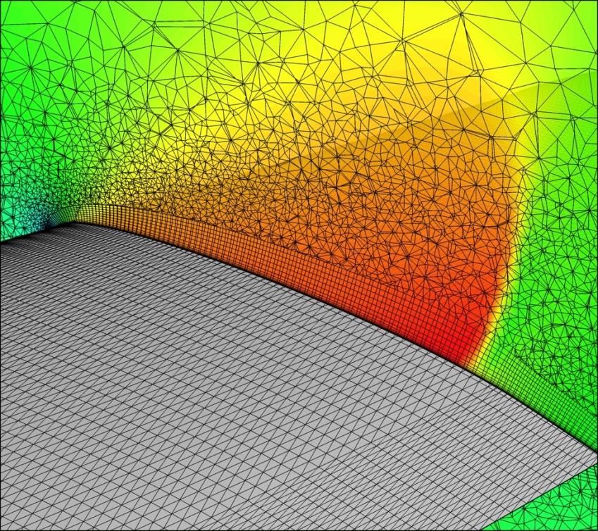
Amazon Web Services Computational Fluid Dynamics on AWS

Introduction
Fluid dynamics is the study of the motion of fluids, usually in the presence of an object.
Typical fluid flows of interest to engineers and scientist include flow in pipes, through
engines, and around objects, such as buildings, automobiles, and airplanes.
Computational fluid dynamics (CFD) is the study of these flows using a numerical
approach. CFD involves the solution of conservation equations (mass, momentum,
energy, and others) in a finite domain.

Many CFD tools are currently available, including specialized and “in-house” tools. This
variety is the result of the broad domain of physical problems solved with CFD. There is
not a universal code for all applications, although there are packages that offer great
capabilities. Broad CFD capabilities are available in commercial packages, such as
ANSYS Fluent, Siemens Simcenter STAR-CCM+, Metacomp Technologies CFD++, and
open-source packages, such as OpenFOAM and SU2.

A typical CFD simulation involves the following four steps.

 • Define the geometry — In some cases, this step is simple, such as modeling
 flow in a duct. In other cases, this step involves complex components and
 moving parts, such as modeling a gas turbine engine. For many cases, the
 geometry creation is extremely time-consuming. The geometry step is graphics
 intensive and requires a capable graphics workstation, preferably with a Graphics
 Processing Unit (GPU). Often, the geometry is provided by a designer, but the
 CFD engineer must “clean” the geometry for input into the flow solver. This can
 be a time-consuming step and can sometimes require a large amount of system
 memory (RAM) depending on the complexity of the geometry.

 • Generate the mesh or grid — Mesh generation is a critical step because
 computational accuracy is dependent on the size, cell location, and skewness of
 the cells. In Figure 1, a hybrid mesh is shown on a slice through an aircraft wing.
 Mesh generation can be iterative with the solution, where fixes to the mesh are
 driven by an understanding of flow features and gradients in the solution.
 Meshing is frequently an interactive process and its elliptical nature generally
 requires a substantial amount of memory. Like geometry definition, generating a
 single mesh can take hours, days, weeks, and sometimes months. Many mesh
 generation codes are still limited to a single node, so general-purpose Amazon
 Elastic Compute Cloud (Amazon EC2) instances, such as the M family, or
 memory-optimized instances, such as the R family, are often used.

 1

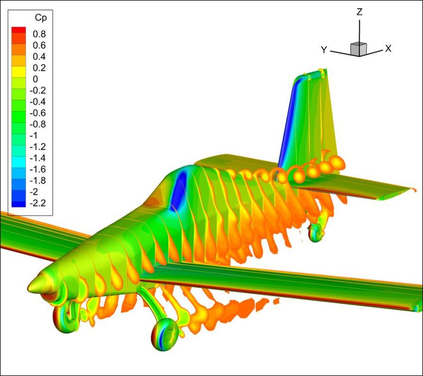
Amazon Web Services Computational Fluid Dynamics on AWS

 Figure 1: Mesh generation

 • Solve for the solution — This step is the primary focus of this whitepaper. For
 some solutions, tens of thousands of cores (processors) run over weeks to
 achieve a solution. Conversely, some jobs may run in just minutes when scaled
 out appropriately. There are choices for model equations depending on the
 desired solution fidelity. The Navier-Stokes equations form the basis of the
 solved equations for most fluid calculations. The addition of chemical reactions,
 liquid and gas multi-phase flows, and many other physical properties create
 increasing complexity. For example, increasing the fidelity of turbulence modeling
 is achieved with various approximate equation sets such as Reynolds Average
 Navier-Stokes (RANS), Large Eddy Simulation (LES), Delayed Detached Eddy
 Simulation (DDES), and Direct Numerical Simulation (DNS). These approaches
 typically do not change the fundamental computational characteristics or scaling
 of the simulation.

 • Post process through visualization — Examples of this step include the
 creation of images, video, and post processing of flow fields, such as creating
 total forces and moments. Similar to the geometry and mesh steps, this can be
 graphics and memory intensive, and graphics processing units (GPUs) are often
 favored.

 2

Amazon Web Services Computational Fluid Dynamics on AWS

 Figure 2: Post-processing visualization

Why CFD on AWS?
AWS is a great place to run CFD cases. CFD workloads are typically tightly coupled
workloads using a Message Passing Interface (MPI) implementation and relying on a
large number of cores across many nodes. Many of the AWS instance types, such as
the compute family instance types, are designed to include support for this type of
workload. AWS has network options that support extreme scalability and short turn-
around time as necessary.

CFD workloads typically scale well on the cloud. Most codes rely on domain
decomposition to distribute portions of the calculation to the compute nodes. A case can
be run highly parallel to receive results in minutes. Additionally, large numbers of cases
can run simultaneously as efficiently and cheaply as possible to allow the timely
completion of all cases.

The cloud offers a quick way to deploy and turn around CFD workloads at any scale
without the need to own your own infrastructure. You can run jobs that once were in the
realm of national labs or large industry. In just an hour or two, you can deploy CFD

 3

Amazon Web Services Computational Fluid Dynamics on AWS

software, upload input files, launch compute nodes, and complete jobs on a large
number of cores. When your job completes, results can be visualized and downloaded,
and then all resources can be ended – so you only pay for what you use. If preferred,
your results can be securely archived on AWS using a storage service, such as Amazon
Simple Storage Service (Amazon S3). Due to cloud scalability, you have the option to
run multiple cases simultaneously with a dedicated cluster for each case.

The cloud accommodates the variable demand of CFD. Often, there is a need to run a
large number of cases as quickly as possible. Situations can require a sudden burst of
tens, hundreds, or thousands of calculations immediately, and then perhaps no runs
until the next cycle. The need to run a large number of cases could be for a preliminary
design review, or perhaps a sweep of cases for the creation of a solution database. On
the cloud, the cost is the same to run many jobs simultaneously, in parallel, as it is to
run them serially, so you can get your data more quickly and at no extra cost. The cost
savings in engineering time is an often-forgotten part of cost analysis. Running in
parallel can be an ideal solution for design optimization.

Cloud computing is a strong choice for other CFD steps. You can easily change the
underlying hardware configuration to handle the geometry, meshing, and post-
processing. With remote visualization software available to handle the display, you can
manage the GPU instance running your post-processing visualization from any screen
(laptop, desktop, web browser) as though you were working on a large workstation.

Getting started with AWS
To begin, you must create an AWS account and an AWS Identity and Access
Management (IAM) user. An IAM user is a user within your AWS account. The IAM user
allows authentication and authorization to AWS resources. Multiple IAM users can be
created if multiple people need access to the same AWS account.

During the first year after account activation, many AWS services are available for free
with the AWS Free Tier. The free-tier program provides an opportunity to learn about
AWS without incurring significant charges. It provides an offset to charges incurred
while training on AWS. However, the compute-heavy nature of CFD means that charges
are regularly not covered by the free tier. Training helps limit mistakes resulting in
unnecessary charges. You can also set up AWS billing alarms to alert you of estimated
charges.

After creating an AWS account, you are provided with what is referred to as your root
user. It is recommended that you do not use this root user for anything other than

 4

Amazon Web Services Computational Fluid Dynamics on AWS

billing. Instead, set up privileged users (through IAM) for day-to-day usage of AWS. IAM
users are useful because they help you securely control access to AWS resources
within your account. Use IAM to control authentication and authorization for resources.
Create IAM users for everyone, including yourself, and preserve the root user for the
required account and service management tasks.

By default, your account is limited on the number of instances that you can launch in a
Region, which is a physical location around the world where AWS clusters data centers.
These limits are initially set low to prevent unnecessary charges, but you can raise them
to preferred values. CFD applications often require a large number of compute
instances simultaneously. The ability and advantages of scaling horizontally are highly
desirable for high performance computing (HPC) workloads. However, you may need to
request an increase to the Amazon EC2 Service Limits before deploying a large
workload to either one large cluster, or too many smaller clusters at once.

If you want to understand more about the underlying services, a few foundational
tutorials can be helpful to get started on AWS:

 • Amazon Elastic Compute Cloud (Amazon EC2) is the Amazon Web Service you
 use to create and run compute nodes in the cloud. AWS calls these compute
 nodes “instances”. This Launch a Linux Virtual Machine with Amazon Lightsail
 tutorial will help you successfully launch a Linux compute node on Amazon EC2
 within our AWS Free Tier.

 • Amazon Simple Storage Service (Amazon S3) is a service that enables you to
 store your data (referred to as objects) at massive scale. This Store and Retrieve
 a File with Amazon S3 tutorial will help you store your files in the cloud using
 Amazon S3 by creating an Amazon S3 bucket, uploading a file, retrieving the file,
 and deleting the file.

 • AWS Command Line Interface (CLI) is a common programmatic tool for
 automating AWS resources. For example, you can use it to deploy AWS
 infrastructure or manage data in S3. In this AWS Command Line Interface
 tutorial, you learn how to use the AWS CLI to access Amazon S3. You can then
 easily build your own scripts for moving your files to the cloud and easily
 retrieving them as needed.

 5

Amazon Web Services Computational Fluid Dynamics on AWS

 • AWS Budgets gives you the ability to set custom budgets that alert you when
 your costs or usage exceed (or are forecasted to exceed) your budgeted amount.
 In the Control your AWS costs With the AWS Free Tier and AWS Budgets
 tutorial, you learn how to control your costs while exploring AWS service
 offerings using the AWS Free Tier then using AWS Budgets to set up a cost
 budget to monitor any costs associated with your usage.

A dedicated Running CFD on AWS workshop has been created to guide you through
the process of running your CFD codes on AWS. This workshop has step-by-step
instructions for common codes like Simcenter STAR-CCM+, OpenFOAM, and ANSYS
Fluent.

Additionally, the AWS Well-Architected Framework High Performance Computing (HPC)
Lens covers common HPC scenarios and identifies key elements to ensure that your
workloads are architected according to best practices. It focuses on how to design,
deploy, and architect your HPC workloads on the AWS Cloud.

CFD approaches on AWS
Most CFD solvers have locality of data and use sparse matrix solvers. Once properly
organized (application dependent), a well-configured job exhibits good strong and weak
scaling on simple AWS cluster architectures. “Structured” and “Unstructured” codes are
commonly run on AWS. Spectral and pseudo-spectral methods involve Fast Fourier
Transforms (FFTs), and while less common than traditional CFD algorithms, they also
scale well on AWS. Your architectural decisions have tradeoffs, and AWS makes it
quick and easy to try different architectures to optimize for cost and performance.

Architectures
There are two primary design patterns to consider when choosing an AWS architecture
for CFD applications: the traditional cluster and the cloud native cluster. Customers
choose their preferred architecture based on the use case and the CFD users’ needs.
For example, use cases that require frequent involvement and monitoring, such as
when you need to start and stop the CFD case several times on the way to
convergence, often prefer a traditional style cluster.

 6

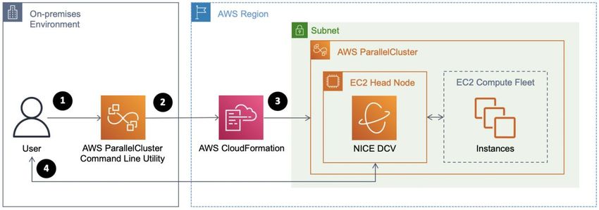
Amazon Web Services Computational Fluid Dynamics on AWS

Conversely, cases that are easily automated often prefer a cloud native setup, which
enables you to easily submit large numbers of cases simultaneously or automate your
run for a complete end-to-end solution. Cloud native is useful when cases require
special pre- or post-processing steps which benefit from automation. Whether choosing
traditional or cloud native architectures, the cloud offers the advantage of elastic
scalability — enabling you to only consume and pay for resources when you need them.

Traditional cluster environments
In the cloud, a traditional cluster is also referred to as a persistent cluster due to the
persistence of minimal AWS infrastructure required for preserving the cluster
environment. Examples of persistent infrastructure include a node running a scheduler
and hosting data even after a completed run campaign. The persistent cluster mimics a
traditional on-premises cluster or supercomputer experience. Clusters include a login
instance with a scheduler that allows multiple users to submit jobs. The compute node
fleet can be a fixed size or a dynamic group to increase and decrease the number of
compute instances depending on the jobs submitted.

AWS ParallelCluster is an example of a persistent cluster that simplifies the deployment
and management of HPC clusters in the AWS Cloud. It enables you to quickly launch
and terminate an HPC compute environment in AWS as needed. AWS ParallelCluster
orchestrates the creation of the required resources (for example, compute nodes and
shared filesystems) and provides an automatic scaling mechanism to adjust the size of
the cluster to match the submitted workload. You can use AWS ParallelCluster with a
variety of batch schedulers, including Slurm and AWS Batch.

 Figure 3: Example AWS ParallelCluster architecture

An AWS ParallelCluster architecture enables the following workflow:

 7

Amazon Web Services Computational Fluid Dynamics on AWS

 • Creating a desired configuration through a text file

 • Launching a cluster through the AWS ParallelCluster Command Line Utility (CLI)

 • Orchestrating AWS services automatically through AWS CloudFormation

 • Accessing the cluster through the command line with Secure Shell Protocol
 (SSH) or graphically with NICE DCV

Cloud native environments
A cloud native cluster is also called an ephemeral cluster due to its relatively short
lifetime. A cloud native approach to tightly coupled HPC ties each run, or sweep of runs,
to its own cluster. For each case, resources are provisioned and launched, data is
placed on the instances, jobs run across multiple instances, and case output is retrieved
automatically or sent to Amazon S3. Upon job completion, the infrastructure is ended.
Clusters designed this way are ephemeral, treat infrastructure as code, and allow for
complete version control of infrastructure changes. Login nodes and job schedulers are
less critical and often not used at all with an ephemeral cluster. The following are a few
frequently used methods to implement such a design:

 • Scripted approach — A common quick-start approach for CFD users getting
 started with AWS is to combine a custom Amazon Machine Image (AMI) with the
 AWS CLI and a bash script. After launching an Amazon EC2 instance, software
 can be added to the instance and an AMI is created to be used as the starting
 point for all compute nodes. It is typical to set up the SSH files and the .bashrc
 file before creating the custom AMI or “golden image.” Although many CFD
 solvers do not require a shared file location, one can easily be created with an
 exported network file system (NFS) volume, or with Amazon FSx for Lustre, an
 AWS managed Lustre file system.
 • API based — If preferred, an automated deployment can be developed with one
 of the Software Development Kits (SDK), such as Python, available for
 programming an end-to-end solution.

 • CloudFormation templates — AWS CloudFormation is an AWS Cloud native
 approach to provisioning AWS resources based on a JSON or YAML template.
 AWS CloudFormation offers an easily version-controlled cluster provisioning
 capability.

 8

Amazon Web Services Computational Fluid Dynamics on AWS

 • AWS Batch — AWS Batch is a cloud-native, container-based approach that
 enables CFD users to efficiently run hundreds of thousands of batch computing
 jobs in containers on AWS. AWS Batch dynamically provisions the optimal
 quantity and type of compute resources (for example, compute or memory-
 optimized instances) based on the volume and specific resource requirements of
 the batch jobs submitted.

 With AWS Batch, there is no need to install and manage batch computing
 software or server infrastructure that you use to run your jobs — enabling you to
 focus on analyzing results and solving problems. AWS Batch plans, schedules,
 and runs your batch computing workloads across the full range of AWS compute
 services and features, such as Amazon EC2 and Spot Instances. AWS Batch
 can also be used as a job scheduler with AWS ParallelCluster.

Software
Installation
CFD software can either be installed into a base AMI, or it can be used from prebuilt
AMIs from the AWS Marketplace. If installing into a base AMI, a custom AMI can be
created to launch new instances with the software already installed. The AWS
Marketplace offers a listing of software from individual software vendors, which offer
software included with AWS services. Finally, you can also add the installation to the
cluster deployment scripts and run them at cluster creation.

Licensing
Many commercial CFD solvers are licensed and may require access to a license server,
such as FlexNet Publisher. Licensing software in the cloud is much like licensing with
any other cluster. If a license server is necessary, you can configure your networking to
use an existing on-premises server, or you can host the license server on the cloud.

If hosting the license server on AWS, burstable general-purpose T instances in small
sizes, such as micro, can be used for cost-effective hosting. A Reserved Instance
purchase for the license server provides further cost savings.

The FlexNet Publisher license relies on the network interface’s MAC address. The
easiest way to retrieve the new MAC address for your license is to launch the instance
and retrieve the MAC address before the license is issued. You can preserve the MAC
address by changing the ending behavior to prevent deletion of the network interface if
the instance is ever terminated. When hosting your own license server, confirm that the

 9

Amazon Web Services Computational Fluid Dynamics on AWS

security group for the license-server instance allows connectivity on the appropriate
ports required by the software package.

If accessing an on-premises license server, create an AWS Site-to-Site VPN for your
Virtual Private Cloud (VPC), or alternatively, if on-premises firewalls allow, you may be
able to access the on-premises license server through SSH tunneling.

Cloud-friendly licensing through power-on-demand licensing keys is also growing in
popularity and relies on submitting a job with a key provided by the software provider.

Setup
There are multiple strategies for setting up software in clusters. The most widely used
examples are below:

Create a custom AMI
This method features the shortest application startup time and avoids potential
bottlenecks when accessing a single shared resource. This is the preferred means of
distribution for large-scale runs (10s of thousands of MPI ranks) or applications that
must load a large number of shared libraries. A drawback is the larger AMI size, which
incurs more cost for Amazon Elastic Block Store (Amazon EBS).

Share an Amazon EBS volume via NFS
This method installs the necessary software into a single Amazon EBS volume, creates
an NFS export on a single instance, and mounts the NFS share on all of the compute
instances. This approach reduces the Amazon EBS footprint because only one Amazon
EBS volume must be created for the software. This method is useful for large software
packages and moderate scale runs (up to thousands of MPI ranks).

To optimize input/output (I/O) performance, different EBS volume types are available
offering different performance characteristics. A tradeoff with this method is a small
amount of added network traffic and a potential bottleneck with a single instance hosting
the NFS share. Ensuring a larger NFS host instance with additional network capabilities
mitigates these concerns.

To make this approach repeatable, the exported NFS directory can be decoupled from
the root volume, stored on a separate Amazon EBS volume, and created from an
Amazon EBS snapshot. This approach is similar to the custom AMI method, but instead
it isolates software from the root volume. An additional Amazon EBS volume is created
from an Amazon EBS snapshot at instance launch and is mounted as an additional disk

 10

Amazon Web Services Computational Fluid Dynamics on AWS

to the compute instance. The snapshot used to create the volume contains the software
installation. Decoupling the user software from operating system updates that are
necessary on the root volume reduces the complexity of maintenance. Furthermore, the
user can rely on the latest AMI releases for the compute instances, which provide an
up-to-date system without maintaining a custom AMI.

Use a managed shared file system
This approach installs the CFD software into an AWS managed file system service,
such as Amazon FSx for Lustre or Amazon Elastic File System (Amazon EFS), and
mounts the shared file system on all of the compute instances. Amazon FSx for Lustre
provides a high-performance, parallel file system optimized for HPC workloads. Lustre
is optimized for simultaneous access, and its performance can be scaled independently
from any single instance size.

FSx for Lustre works natively with Amazon S3 and can be automatically populated with
data residing in S3, which enables users to have a Lustre file system running only while
compute jobs are active and easily discard it afterwards.

EFS provides a simple, scalable, fully managed elastic NFS file system that can be
used as a location for home directories. However, EFS is not recommended for other
aspects of a CFD cluster, such as hosting simulation data or compiling a solver, due to
performance considerations.

Maintenance
New feature releases and patches to existing software are a frequent need in the CFD
application workflow. All distribution strategies can be fully automated. When using the
AMI or Amazon EBS snapshot strategy, the software update cycle can be isolated from
the application runs. Once a new AMI or snapshot has been created and tested, the
cluster is reconfigured to pick up the latest version. Software updates cycles in the
strategies using file sharing via NFS or FSx for Lustre must be coordinated with
application runs because a live system is being altered.

In general, automating CFD application installation with scripting tools is recommended
and is usually referred to as a Continuous Integration/Continuous Deployment (CI/CD)
pipeline on AWS. The automation process eliminates the manual processes required to
build and deploy new software and security patches to HPC systems. This is useful if
you want to use the latest features in software packages with fast update cycles. You
can read more about CI/CD pipelines in the AWS Continuous Delivery documentation.

 11

Amazon Web Services Computational Fluid Dynamics on AWS

Cluster lifecycle
AWS offers a variety of unique ways to design architectures that deploy HPC
workloads. Your choice of deployment method for a particular workload depends on a
number of factors, including your desired user experience, degree of automation,
experience with AWS, preferred scripting languages, size and number of cases, and the
lifecycle of your data. The High Performance Computing Lens whitepaper covers
additional best practices for architectures beyond what is discussed in this paper.

While the architecture for a cluster is typically unique and tailored for the workload, all
HPC clusters benefit from lifecycle planning and management of the cluster and the
data produced — allowing for optimized performance, reliability, and cost.

It is not unusual for an on-premises cluster to run for many years, perhaps without
significant operating system (OS) update or modification, until the hardware is obsolete
thus rendering it useless. In contrast, AWS regularly releases new services and updates
to improve performance and lower costs. The easiest way to take advantage of new
AWS capabilities, such as new instances, is by maintaining the cluster as a script or
template. AWS refers to this as “Infrastructure as Code” because it allows for the
creation of clusters quickly, provides repeatable automation, and maintains reliable
version control.

Examples of “cluster as code” are the AWS ParallelCluster configuration file,
deployment scripts, or CloudFormation templates. These text-based configurations are
easy to modify for a new capability or workload.

A view of the cluster lifecycle includes infrastructure as code that starts before the
cluster is deployed with the maintenance of the deployment scripts. Elements of a
cluster maintained as code include:

 • Base AMI to build your cluster
 • Automated software installation scripts

 • Configuration files, such as scheduler configs, MPI configurations, and .bashrc

 • Text description of the infrastructure, such as a CloudFormation template, or an
 AWS ParallelCluster configuration file

 • Script to initiate cluster deployment and subsequent software installation

While the nature of a cluster changes depending on the type of workload, the most cost-
effective clusters are those that are deployed only when they are actively being used.

 12

Amazon Web Services Computational Fluid Dynamics on AWS

The cluster lifecycle can have a significant impact on costs. For example, it is common
with many traditional on-premises clusters to maintain a large storage volume. This is
not necessary in the cloud because data can be easily moved to S3 where it is reliably
and cheaply stored. Maintaining a cluster as code allows you to place a cluster under
version control and repeatedly deploy replicas if needed.

Each cluster maintained as code can be instantiated multiple times if multiple clusters
are required for testing, onboarding new users, or running a large number of cases in
parallel. If set up correctly, you avoid idle infrastructure when jobs are not running.

CFD case scalability
CFD cases that cross multiple nodes raise the question, “How will my application scale
on AWS?” CFD solvers depend heavily on the solver algorithm’s ability to scale
compute tasks efficiently in parallel across multiple compute resources. Parallel
performance is often evaluated by determining an application’s scale-up. Scale-up is a
function of the number of processors used and is defined as the time it takes to
complete a run on one processor, divided by the time it takes to complete the same run
on the number of processors used for the parallel run.

 1 
 ( ) =
 
Scaling is considered to be excellent when the scale-up is close to or equal to the
number of processors on which the application is run. An example of scale up as a
function of core count is shown in Figure 4.

 13

Amazon Web Services Computational Fluid Dynamics on AWS

 1000

 900

 800

 700

 600
 Scale-Up

 500

 400

 300 Ideal
 c5n
 200

 100

 0
 0 200 400 600 800 1000
 Cores

 Figure 4: Strong scaling demonstrated for a 14M cell external aerodynamics use case

The example case in Figure 4 is a 14 million cell external aerodynamics calculation
using a cell-centered unstructured solver. The mesh is composed largely of hexahedra.
The black line shows the ideal or perfect scalability. The blue diamond-based curve
shows the actual scale-up for this case as a function of increasing processor count.
Excellent scaling is seen to almost 1000 cores for this small sized case. This example
was run on Amazon EC2 c5n.18xlarge instances, with Elastic Fabric Adapter (EFA),
and using a fully loaded compute node.

For this calculation, all cores are fully utilized, meaning that no core was left idle during
the calculation. Most customers like to use the entire instance when running a
calculation. Faster turn-around times can be achieved by reducing the number of
processes on each instance.

Fourteen million cells is a relatively small CFD case by today’s standards. A small case
was purposely chosen for the discussion on scalability because small cases are more
difficult to scale. The idea that small cases are harder than large cases to scale may

 14

Amazon Web Services Computational Fluid Dynamics on AWS

seem counter intuitive, but smaller cases have less total compute to spread over a large
number of cores. An understanding of strong scaling vs. weak scaling offers more
insight.

Strong scaling vs. weak scaling
Case scalability can be characterized two ways: strong scaling or weak scaling. Weak
does not mean inadequate — it is a technical term facilitating the description of the type
of scaling.

Strong scaling, as demonstrated in Figure 4, is a traditional view of scaling, where a
problem size is fixed and spread over an increasing number of processors. As more
processors are added to the calculation, good strong scaling means that the time to
complete the calculation decreases proportionally with increasing processor count.

In comparison, weak scaling does not fix the problem size used in the evaluation, but
purposely increases the problem size as the number of processors also increases. The
ratio of the problem size to the number of processors on which the case is run is
constant. For a CFD calculation, problem size most often refers to the number of cells
or nodes in the mesh for a similar configuration.

An application demonstrates good weak scaling when the time to complete the
calculation remains constant as the ratio of compute effort to the number of processors
is held constant. Weak scaling offers insight into how an application behaves with
varying case size. Well-written CFD solvers offer excellent weak scaling capability
allowing for more cores to be used when running bigger applications. The scalability of
CFD cases can then be determined by looking at a normalized plot of scale-up based
on the number of mesh cells per core (cells/core). An example plot is shown in Figure 5.

 15

Amazon Web Services Computational Fluid Dynamics on AWS

 1000

 900 100%

 800
 90%
 700

 600

 Efficiency
 80%
 Scale-up

 500

 400
 70%
 300

 200 60%
 Scale-Up
 100
 Efficiency
 0 50%
 200,000 150,000 100,000 50,000 0
 Cells/Core

 Figure 5: Scale-up and efficiency as a function of cells per processor

Running efficiency
Efficiency is defined as the scale-up divided by the number of processors used in the
calculation. Scale-up and efficiency as a function of cells/core is shown in Figure 5. In
Figure 5, the cells per core are on the horizontal axis. The blue line in Figure 5 shows
scale-up as a function of mesh cells per processor. The vertical axis for scale-up is on
the left-hand side of the graph as indicated by the blue arrow. The orange line in Figure
5 shows efficiency as a function of mesh cells per core. The vertical axis for efficiency is
shown on the right side of the graph and is indicated by an orange arrow.

 ( ) = ∗ 100
 
For similar case types, running with similar solver settings, a plot like the one in Figure 5
can help you choose the desired efficiency and number of cores running for a given
case.

 16

Amazon Web Services Computational Fluid Dynamics on AWS

Efficiency remains at about 100% between approximately 200,000 mesh cells per core
and 100,000 mesh cells per core. Efficiency starts to fall off at about 50,000 mesh cells
per core. An efficiency of at least 80% is maintained until 20,000 mesh cells per core,
for this case. Decreasing mesh cells per core leads to decreased efficiency because the
total computational effort per core is reduced. The inefficiencies that show up at higher
core counts come from a variety of sources and are caused by “serial” work. Serial work
is the work that cannot be effectively parallelized. Serial work comes from solver
inefficiencies, I/O inefficiencies, unequal domain decomposition, additional physical
modeling such as radiative effects, and eventually, from the network as core count
continues to increase.

Turn-around time and cost
Plots of scale-up and efficiency offer an understanding about how a case or application
scales. However, what matters most HPC users is case turn-around time and cost. A
plot of turn-around time versus CPU cost for this case is shown in Figure 6. As the
number of cores increases, the inefficiency also increases, which leads to increased
costs.

 17

Amazon Web Services Computational Fluid Dynamics on AWS

 $8.00

 20,000 Cells/Core
 $7.00
 Cost for 1000 Iterations

 $6.00

 50,000 Cells/Core
 200,000 Cells/Core
 $5.00

 $4.00
 0 10 20 30 40 50
 Turn-Around Time (Minutes)

 Figure 6: Cost for per run based on on-demand pricing for the c5n.18xlarge instance as a
 function of turn-around time

In Figure 6, the turn-around time is shown on the horizontal axis. The cost is shown on
the vertical axis. The price is based on the “on-demand” price of a c5n.18xlarge for
1000 iterations, and only includes the computational costs. Small costs are also
incurred for data storage. Minimum cost was obtained at approximately 50,000 cells per
core or more. As the efficiency is 100% over a range of core counts, the price is the
same regardless of the number of cores. Many users choose a cell count per core to
achieve the lowest possible cost.

As core count goes up, inefficiencies start to show up, but turn-around time continues to
drop. When a fast turn-around is needed, users may choose a large number of cores to
accelerate the time to solution. For this case, a turn-around time of about five minutes
can be obtained by running on about 20,000 cells per core. When considering total cost,
the inclusion of license costs may make the fastest run the cheapest run.

 18

Amazon Web Services Computational Fluid Dynamics on AWS

Optimizing HPC components
The AWS Cloud provides a broad range of scalable, flexible infrastructure services that
you select to match your workloads and tasks. This gives you the ability to choose the
most appropriate mix of resources for your specific applications. Cloud computing
makes it easy to experiment with infrastructure components and architecture design.
The HPC solution components listed below are a great starting point to set up and
manage your HPC cluster. Always test various solution configurations to find the best
performance at the lowest cost.

Compute
The optimal compute solution for a particular HPC architecture depends on the
workload deployment method, degree of automation, usage patterns, and configuration.
Different compute solutions may be chosen for each step of a process. Selecting the
appropriate compute solution for an architecture can lead to higher performance
efficiency and lower cost.

There are multiple compute options available on AWS, and at a high level, they are
separated into three categories: instances, containers, and functions. Amazon EC2
instances, or servers, are resizable compute capacity in the cloud. Containers provide
operating system virtualization for applications that share an underlying operating
system installed on a server. Functions are a serverless computing model that allows
you to run code without thinking about provisioning and managing the underlying
servers. For CFD workloads, EC2 instances are the primary compute choice.

Amazon EC2 lets you choose from a variety of compute instance types that can be
configured to suit your needs. Instances come in different families and sizes to offer a
wide variety of capabilities. Some instance families target specific workloads, for
example, compute-, memory-, or GPU-intensive workloads, while others are general
purpose. Both the targeted-workload and general-purpose instance families are useful
for CFD applications based on the step in the CFD process.

When considering CFD steps, different instance types can be targeted for pre-
processing, solving, and post-processing. In pre-processing, the geometry step can
benefit from an instance with a GPU, while the mesh generation stage may require a
higher memory-to-core ratio, such as general-purpose or memory-optimized instances.
When solving CFD cases, evaluate your case size and cluster size.

 19

Amazon Web Services Computational Fluid Dynamics on AWS

If the case is spread across multiple instances, the memory requirements are low per
core, and compute-optimized instances are recommended as the most cost-effective
and performant choice. If a single-instance calculation is desired, it may require more
memory per core and benefit from a general-purpose, or memory-optimized instance.

Optimal performance is typically obtained with compute-optimized instances (Intel,
AMD, or Graviton), and when using multiple instances with cells per core below
100,000, instances with higher network throughput and packet rate performance are
preferred. Refer to the Instance Type Matrix for instance details.

AWS enables simultaneous multithreading (SMT), or hyper-threading technology for
Intel processors, commonly referred to as “hyperthreading” by default for supported
processors. Hyperthreading improves performance for some systems by allowing
multiple threads to be run simultaneously on a single core. Most CFD applications do
not benefit from hyperthreading, and therefore, disabling it tends to be the preferred
environment. Hyperthreading is easily disabled in Amazon EC2. Unless an application
has been tested with hyperthreading enabled, it is recommended that hyperthreading be
disabled and that processes are launched and pinned to individual cores.

There are many compute options available to optimize your compute environment.
Cloud deployment allows for experimentation on every level from operating system to
instance type to bare-metal deployments. Time spent experimenting with cloud-based
clusters is vital to achieving the desired performance.

Network
Most CFD workloads exceed the capacity of a single compute node and require a
cluster-based solution. A crucial factor in achieving application performance with a
multi-node cluster is optimizing the performance of the network connecting the compute
nodes.

Launching instances within a cluster placement group provides consistent, low latency
within a cluster. Instances launched within a cluster placement group are also launched
to the same Availability Zone.

To further improve the network performance between EC2 instances, you can use an
Elastic Fabric Adapter (EFA) on select instance types. EFA is designed for tightly
coupled HPC workloads by providing an OS-bypass capability and hardware-designed
reliability to take advantage of the EC2 network. It works well with CFD solvers. OS-
bypass is an access model that allows an application to bypass the operating system’s
TCP/IP stack and communicate directly with the network device. This provides lower

 20

Amazon Web Services Computational Fluid Dynamics on AWS

and more consistent latency and higher throughput than the TCP transport traditionally
used. When using EFA, your normal IP traffic remains routable and can communicate
with other network resources.

CFD applications use EFA through an MPI implementation using the Libfabric API. To
confirm that EFA is available, query the list of available fabric providers with the
following command:

 $ fi_info -p efa
 provider: efa
 fabric: EFA-fe80::94:3dff:fe89:1b70
 domain: efa_0-rdm
 version: 2.0
 type: FI_EP_RDM
 protocol: FI_PROTO_EFA
 provider: efa
 fabric: EFA-fe80::94:3dff:fe89:1b70
 domain: efa_0-dgrm
 version: 2.0
 type: FI_EP_DGRAM
 protocol: FI_PROTO_EFA
 provider: efa;ofi_rxd
 fabric: EFA-fe80::94:3dff:fe89:1b70
 domain: efa_0-dgrm
 version: 1.0
 type: FI_EP_RDM
 protocol: FI_PROTO_RXD

The command will return information about available EFA interfaces through Libfabric. If
EFA is available, its usage can be confirmed with the MPI runtime debugging output.
Each MPI implementation has environment variables or command line flags for verbose
debugging output or explicitly setting the fabric provider. These options vary by MPI
implementation, and access to these options vary by CFD application. See Getting
Started with EFA and MPI documentation for additional details.

Storage
AWS provides many storage options for CFD, including object storage with Amazon S3,
block storage with Amazon EBS, temporary block-level storage with Amazon EC2
instance store, and file storage with Amazon FSx for Lustre. You can utilize all these
storage types for certain aspects of your CFD workload.

 21

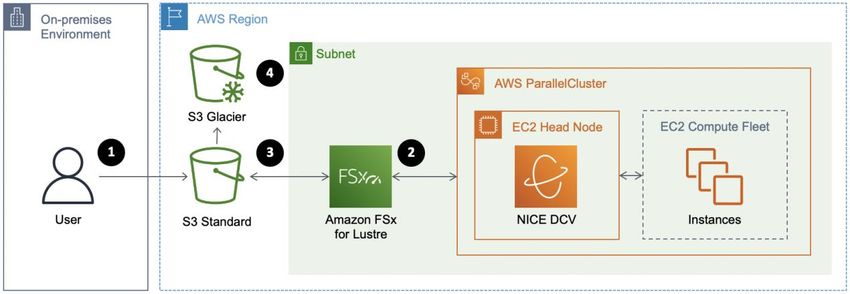
Amazon Web Services Computational Fluid Dynamics on AWS

A vital part of working with CFD solvers on AWS is the management of case data, which
includes files such as CAD, meshes, input files, and output figures. In general, all CFD
users want to maintain availability of the data when it is in use and to archive a subset
of the data if it’s needed at some point in the future.

An efficient data lifecycle uses a combination of storage types and tiers to minimize
costs. Data is described as hot, warm, and cold, depending on the immediate need of
the data.

 • Hot data is data that you need immediately, such as a case or sweep of cases
 about to be deployed.
 • Warm data is your data, which is not needed at the moment, but it may be used
 sometime in the near future; perhaps within the next six months.

 • Cold data is data that may not ever be used again, but it is stored for archival
 purposes.

Your data lifecycle can occur only within AWS, or it can be combined with an on-
premises workflow. For example, you may move case data, such as a case file, from
your local computing facilities, to Amazon S3, and then to an EC2 cluster. Completed
runs can traverse the same path in reverse back to your on-premises environment or to
Amazon S3 where they can remain in the S3 Standard or S3 Infrequent Access storage
class, or transitioned to Amazon S3 Glacier through a lifecycle rule for archiving.
Amazon S3 Glacier and S3 Glacier Deep Archive are S3 storage tiers that offer deep
discounts on storage for archival data. Figure 7 is an example data lifecycle for CFD.

 Figure 7: Data lifecycle

 1. Transferring input data to AWS
 2. Running your simulation with input (hot) data

 22

Amazon Web Services Computational Fluid Dynamics on AWS

 3. Storing your output (warm) data
 4. Archiving inactive (cold) data

Transferring input data
Input data, such as a CAD file, may start on-premises and be transferred to AWS. Input
data is often transferred to Amazon S3 and stored until you are ready to run your
simulation. S3 offers highly scalable, reliable, durable, and secure storage. An S3
workflow decouples storage from your compute cluster and provides a cost-effective
approach. Alternatively, you can transfer your input data to an existing file system at
runtime. This approach is generally slower and less cost effective when compared to S3
because it requires more expensive resources, such as compute instances or managed
file systems, to be running for the duration of the transfer.

For the data transfer, you can choose a manual, scripted, or managed approach.
Manual and scripted approaches can use the AWS CLI for transferring data to S3,
which helps optimize the data transfer to S3 by running parallel uploads. A managed
approach can use a service, such as AWS DataSync, to move input data to AWS. AWS
DataSync makes it simple and fast to move large amounts of data online between on-
premises storage and Amazon S3.

Running your CFD simulation
Input data for your CFD simulation is considered “hot” data when you are ready to run
your simulation. This data is often accessed in a shared file system or placed on the
head node if the CFD application does not require a shared drive.

If your CFD workload requires a high-performance file system, Amazon FSx for Lustre
is highly recommended. FSx for Lustre works natively with Amazon S3, making it easy
for you to access the input data that is already stored in S3. When linked to an S3
bucket, an FSx for Lustre file system transparently presents S3 objects as files and
allows you to write results back to S3.

During the simulation, you can periodically checkpoint and write intermediate results to
your S3 data repository. FSx for Lustre automatically transfers Portable Operating
System Interface (POSIX) metadata for files, directories, and symbolic links (symlinks)
when importing and exporting data to and from the linked data repository on S3. This
allows you to maintain access controls and restart your workload at any time using the
latest data stored in S3.

 23

Amazon Web Services Computational Fluid Dynamics on AWS

When your workload is done, you can write final results from your file system to your S3
data repository and delete your file system.

Storing output data
Output data from your simulation is considered “warm” data after the simulation finishes.
For a cost-effective workflow, transfer the output data off of your cluster and terminate
the more expensive compute and storage resources. If you stored your data in an
Amazon EBS volume, transfer your output data to S3 with the AWS CLI. If you used
FSx for Lustre, create a data repository task to manage the transfer of output data and
metadata to S3 or export your files with HSM commands. You can also periodically
push the output data to S3 with a data repository task.

Archiving inactive data
After your output data is stored in S3 and is considered cold or inactive, transition it to a
more cost-effective storage class, such as Amazon S3 Glacier and S3 Glacier Deep
Archive. These storage classes allow you to archive older data more affordably than
with the S3 Standard storage class. Objects in S3 Glacier and S3 Glacier Deep Archive
are not available for real-time access and must be restored if needed. Restoring objects
incurs a cost, and to keep costs low yet suitable for varying needs, S3 Glacier and S3
Glacier Deep Archive provide multiple retrieval options.

Storage summary
Use the following table to select the best storage solution for your workload:

 Table 1 — Storage services and their uses

 Service Description Use

 Amazon EBS Block storage Block storage or export as a Network File System (NFS)
 share

 Amazon FSx Managed Fast parallel high-performance file system optimized for
 for Lustre Lustre HPC workloads

 Amazon S3 Object storage Store case files, input, and output data

 Amazon S3 Archival Long-term storage of archival data
 Glacier storage

 24

Amazon Web Services Computational Fluid Dynamics on AWS

 Amazon EFS Managed NFS Network File System (NFS) to share files across multiple
 instances. Occasionally used for home directories. Not
 generally recommended for CFD cases.

Visualization
A graphical interface is useful throughout the CFD solution process, from building
meshes, debugging flow-solution errors, and visualizing the flow field. Many CFD
solvers include visualization packages as part of their installation. As an example,
ParaView is packaged with OpenFOAM. In addition to visualization tools within the CFD
suites, there are third-party visualization tools, which can be more powerful, adaptable,
and general.

Visualization is often performed remotely with either an application that supports client-
server mode or with remote visualization of the server desktop. Client-server mode
works well on AWS and can be implemented in the same way as other remote desktop
set-ups. When using client-server mode for an application, it is important to connect to
the server using the public IP address and not the private IP address, unless you have
private network connectivity configured, such as a Site-to-Site VPN.

AWS offers NICE DCV for local display of remote desktops. NICE DCV is easy to
implement and is free to use with EC2. There are a variety of ways to add NICE DCV to
your HPC cluster. The simplest approach is to launch AWS ParallelCluster. If you are
using AWS ParallelCluster, you can enable NICE DCV on the head node when
launching the cluster with a short addition in the configuration file. A graphics-intensive
instance can be easily launched running a Linux or Windows NICE DCV AMI to have
NICE DCV pre-installed. Refer to Getting Started with NICE DCV on Amazon EC2 for
more information.

AWS also offers managed desktop and application streaming services, such as Amazon
WorkSpaces or Amazon AppStream 2.0. Amazon WorkSpaces is a Desktop-as-a-
Service solution providing Linux or Windows desktops while Amazon AppStream 2.0 is
a non-persistent application and desktop streaming service for Windows environments.

In general, visualizing CFD results on AWS reduces the need to download large data
back to on-premises storage, and it helps reduce cost and increase productivity.

 25

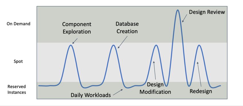
Amazon Web Services Computational Fluid Dynamics on AWS

Costs
AWS offers a pay-as-you-go approach for pricing for cloud services. You pay only for
the individual services you need, for as long as you use them, without long-term
contracts or complex licensing. Some services and tools come free of charge, such as
AWS ParallelCluster, AWS Batch, and AWS CloudFormation; however, the underlying
AWS components used to run cases incur charges.

AWS charges arise primarily from the compute resources required for the CFD solution.
Storage and data transfer also incur charges. Depending on your implementation, you
may use additional services in your architecture, such as AWS Lambda, Amazon
Simple Notification Service (Amazon SNS), or Amazon CloudWatch, but cost
accumulated by usage of these services is rarely significant when compared to the
compute costs for CFD.

It is common to stand up a cluster for only the time period in which it is needed. In a
simple scenario, costs are associated with EC2 instances and Amazon EBS volumes.
Costs incurred after shut down of the cluster include any snapshots taken of Amazon
EBS volumes and any data stored on Amazon S3.

While data transfer into Amazon EC2 from the internet is free, data transfer out of AWS
can incur modest charges. Many users choose to leave their data in S3 and only move
the smaller post-processed data out of AWS. Data can also be transitioned to Amazon
S3 Glacier for archival storage to reduce long-term storage costs.

When AWS ParallelCluster is maintained for an extended period of time, the login node
and Amazon EBS volumes continue to incur costs. The compute nodes scale up and
down as needed, which minimizes costs to only reflect the times when the cluster is
being used.

When developing an architecture, you must monitor your workload (automatically
through monitoring solutions or manually through the console) and ensure that your
resources scale up and down as expected. Occasionally, hung jobs or other factors can
prevent your resources from scaling properly. Logging on to the compute node and
checking processes with a tool, such as top or htop, can help debug issues.

AWS provides four different ways to pay for EC2 instances:

 • On-Demand Instances

 • Reserved Instances

 26

Amazon Web Services Computational Fluid Dynamics on AWS

 • Savings Plans

 • Spot Instances

Amazon EC2 instance costs can be minimized by using Spot Instances, Savings Plans,
and Reserved Instances.

 • On-Demand Instances — With On-Demand Instances, you pay for compute
 capacity by the hour or the second, depending on which you run. No long-term
 commitments or upfront payments are needed. You can increase or decrease
 your compute capacity depending on the demands of your application and only
 pay the specified per-hour rates for the instance you use.

 On-Demand Instances are the highest cost model for computing and require no
 upfront commitment. Cost saving is gained because costs are only incurred while
 the instances are in a running state. For a dynamic workload, the savings can be
 large. Savings occur because you can select the newest processor types, which
 may speed up the computations significantly.

 • Reserved Instances — Reserved Instances (RIs) provide you with a significant
 discount (up to 75%) compared to On-Demand Instance pricing. For customers
 that have steady state or predictable usage and can commit to using EC2 over a
 1- or 3-year term, Reserved Instances provide significant savings compared to
 using On-Demand Instances.

 • Savings Plans — Savings Plans are a flexible pricing model that provides
 savings of up to 72% on your AWS compute usage. This pricing model offers
 lower prices on Amazon EC2 instances usage, regardless of instance family,
 size, OS, tenancy or AWS Region, and also applies to AWS Fargate usage.

 Savings Plans offer significant savings over On-Demand Instances, just like EC2
 Reserved Instances, in exchange for a commitment to use a specific amount of
 compute power (measured in $/hour) for a one- or three-year period. You can
 sign up for Savings Plans for a one- or three-year term and easily manage your
 plans by taking advantage of recommendations, performance reporting, and
 budget alerts in the AWS Cost Explorer.

 27