Extreme-Scale UQ for Bayesian Inverse Problems Governed by PDEs
←
→
Page content transcription
If your browser does not render page correctly, please read the page content below
Extreme-Scale UQ
  for Bayesian Inverse Problems Governed by PDEs
                                    Tan Bui-Thanh∗ , Carsten Burstedde∗† , Omar Ghattas∗‡ ,
                                      James Martin∗ , Georg Stadler∗ , Lucas C. Wilcox∗§
         ∗ Institute
                  for Computational Engineering and Sciences (ICES), The University of Texas at Austin, Austin, TX
        † Now at Institute for Numerical Simulation, Rheinische Friedrich-Wilhelms-Universität Bonn, Bonn, Germany
‡ Jackson School of Geosciences, and Department of Mechanical Engineering, The University of Texas at Austin, Austin, TX
                  § Now at Department of Applied Mathematics, Naval Postgraduate School, Monterey, CA

   Abstract—Quantifying uncertainties in large-scale simulations     erate), conventional uncertainty quantification methods fail
has emerged as the central challenge facing CS&E. When the           dramatically. Here we address uncertainty quantification (UQ)
simulations require supercomputers, and uncertain parameter          in large-scale inverse problems governed by PDEs. This is
dimensions are large, conventional UQ methods fail. Here we
address uncertainty quantification for large-scale inverse prob-     the crucial step in UQ: before we can propagate parameter
lems in a Bayesian inference framework: given data and model         uncertainties forward through a model, we must first infer
uncertainties, find the pdf describing parameter uncertainties. To   them from observational data and from the (PDE) model
overcome the curse of dimensionality of conventional methods,        that maps parameters to observables; i.e., we must solve the
we exploit the fact that the data are typically informative about    inverse problem. We adopt the Bayesian inference framework
low-dimensional manifolds of parameter space to construct low
rank approximations of the covariance matrix of the posterior        [2], [3]: given observational data and their uncertainty, the
pdf via a matrix-free randomized method. We obtain a method          governing forward PDEs and their uncertainty, and a prior
that scales independently of the forward problem dimension,          probability distribution describing prior uncertainty in the
the uncertain parameter dimension, the data dimension, and the       parameters, find the posterior probability distribution over
number of cores. We apply the method to the Bayesian solution        the parameters, which is seen as the solution of the inverse
of an inverse problem in 3D global seismic wave propagation with
over one million uncertain earth model parameters, 630 million       problem. The grand challenge in solving statistical inverse
wave propagation unknowns, on up to 262K cores, for which we         problems is in computing statistics of the posterior probability
obtain a factor of over 2000 reduction in problem dimension.         density function (pdf), which is a surface in high dimensions.
This makes UQ tractable for the inverse problem.                     This is notoriously challenging for statistical inverse problems
                                                                     governed by expensive forward models (as in our target case
                        I. I NTRODUCTION
                                                                     of global seismic wave propagation) and high-dimensional
   Perhaps the central challenge facing the field of computa-        parameter spaces (as in our case of inferring a heteroge-
tional science and engineering today is: how do we quantify          neous parameter field). The difficulty stems from the fact
uncertainties in the predictions of our large-scale simula-          that evaluation of the probability of each point in parameter
tions, given limitations in observational data, computational        space requires solution of the forward problem (which may
resources, and our understanding of physical processes [1].          tax contemporary supercomputers), and many such evaluations
For many societal grand challenges, the “single point” de-           (millions or more) are required to adequately sample the
terministic predictions delivered by most contemporary large-        posterior density in high dimensions by conventional Markov-
scale simulations of complex systems are just a first step: to       chain Monte Carlo (MCMC) methods. Thus, UQ for the large-
be of value for decision-making (design, control, allocation         scale inverse problems becomes intractable.
of resources, policy-making, etc.), they must be accompanied            The approach we take is based on a linearization of the
by the degree of confidence we have in the predictions.              parameter-to-observable map, which yields a local Gaussian
Examples of problems for which large-scale simulations are           approximation of the posterior. The mean and covariance of
playing an increasingly important role for decision-making           this Gaussian can be found from an appropriately weighted
include: mitigation of global climate change, natural hazard         regularized nonlinear least squares optimization problem,
forecasts; siting of nuclear waste repositories, monitoring          which is known as the maximum a posteriori (MAP) point.
of subsurface contaminants, control of carbon sequestration          The solution of this optimization problem provides the mean,
processes, management of the nuclear fuel cycle, design of           and the inverse of the Hessian matrix of the least squares
new nano-structured materials and energy storage systems, and        function (evaluated at the MAP point) gives the covariance
patient-specific planning of surgical procedures, to name a few.     matrix. Unfortunately, the most efficient algorithms available
   Unfortunately, when the simulations (here assumed without         for direct computation of the (nominally dense) Hessian are
loss of generality to comprise PDEs) are expensive, and the          prohibitive, requiring as many forward PDE-like solves as
uncertain parameter dimension is large (or even just mod-            there are uncertain parameters, which can number in the

SC12, November 10-16, 2012, Salt Lake City, Utah, USA
978-1-4673-0806-9/12/$31.00 c 2012 IEEE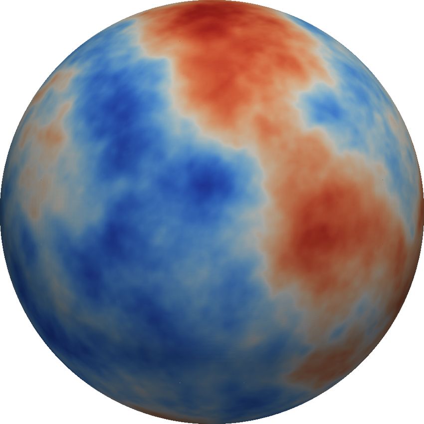
millions or more when the parameter represents a field (e.g,         II. BAYESIAN F ORMULATION OF I NVERSE P ROBLEMS
initial condition, heterogeneous material coefficient, source         In the Bayesian approach, we state the inverse problem as
term).                                                             a problem of statistical inference over the space of uncertain
   The key insight to overcoming this barrier is that the data     parameters, which are to be inferred from the data and a PDE
are typically informative about a low dimensional manifold of      model. The resulting solution to the statistical inverse problem
the parameter space [4]—that is, the Hessian of the data-misfit    is a posterior distribution that assigns to any candidate set of
term in the least squares function is sparse with respect to       parameter fields our belief (expressed as a probability) that a
some basis. We exploit this fact to construct a low rank approx-   member of this candidate set is the “true” parameter field that
imation of the data-misfit Hessian and the resulting posterior     gave rise to the observed data. When discretized, this problem
covariance matrix using a parallel, matrix-free randomized         of infinite dimensional inference gives rise naturally to a large
algorithm, which requires a dimension-independent number of        scale problem of inference over the discrete parameter space
forward PDE solves and associated adjoint PDE solves (the          x ∈ Rn , corresponding to degrees of freedom in the parameter
latter resemble the forward PDEs in reverse time). UQ thus         field mesh. While the presentation in this paper is limited to the
reduces to solving a fixed (and often small, relative to the       finite dimensional approximation to the infinite dimensional
parameter dimension) number of PDEs. When scalable solvers         measure, the discretization process is performed rigorously
are available for the forward PDEs, the entire process of          following [6], [7], and the numerical evidence indicates that
quantifying uncertainties in the solution of the inverse problem   we converge to the correct infinite dimensional distribution.
is scalable with respect to PDE state variable dimension,             The posterior probability distribution combines the prior
uncertain parameter dimension, observational data dimension,       pdf πprior (x) over the parameter space, which encodes any
and number of processor cores. We apply this method to             knowledge or assumptions about the parameter space that we
the Bayesian solution of an inverse problem in 3D global           may wish to impose before the data are considered, with a
seismic wave propagation with 1.067 million parameters and         likelihood pdf πlike (y obs |x), which explicitly represents the
630 million wave propagation spatial unknowns over 2400            probability that a given set of parameters x might give rise to
time steps, on up to 262,144 Jaguar cores. The example             the observed data y obs ∈ Rm . Bayes’ Theorem then explicitly
demonstrates independence of parameter dimension and a             computes the posterior pdf as
factor of over 2000 reduction in problem dimension. This UQ
computation is orders of magnitude larger than any attempted                    πpost (x|y obs ) ∝ πprior (x)πlike (y obs |x).
before on a large-scale forward problem.                              We choose the prior distribution to be Gaussian, with a
   We recently presented a finite-dimensional version of our       covariance operator defined by the square of the inverse of
method (in which Lanczos iterations are used to build the          an elliptic PDE operator. This choice yields several benefits.
low rank approximation of the Hessian) and applied it to a         First, it enables implicit representation of the prior covariance
1D inverse problem in moderate dimensions [5]. We have             operator as (the inverse of) a sparse operator, as opposed
also recently described the extension to infinite-dimensional      to traditional approaches that either store a dense covariance
inverse problems (so-called because the inversion parameters       matrix or its approximation by principle vectors. Second, since
represent a field) in the framework of [6], in which we discuss    the covariance operator is never needed explicitly—only its
mathematically subtle yet critical issues related to the proper    action on a vector is required— we are able to capitalize
choice of prior and to discretizations that assure convergence     on fast O(n) parallel elliptic solvers (in this paper, algebraic
to the correct infinite-dimensional quantities [7]. In this, our   multigrid) to form this action via two elliptic solves. Third,
Bell Prize submission in the Scalable Algorithms category, we      the action of the symmetric square root factorization of the
extend the method to extreme-scale Bayesian inverse prob-          prior covariance is available explicitly (via one elliptic solve
lems, employing a randomized parallel matrix-free low rank         instead of two). Finally, this choice of covariance is useful for
approximation method, instead of Lanczos. The randomized           technical reasons, as it guarantees that samples from the prior
method yields a low rank approximation with controllably           distribution will be continuous.
high probability, and is asynchronous, more robust, more              The difference between the observables predicted by the
fault tolerant, and provides better cache performance. In the      model and the actual observations y obs is due to both mea-
following sections, we provide an overview of the Bayesian         surement and model errors, and is represented by the i.i.d.
formulation of inverse problems (§II), describe how the mean       Gaussian random variable “noise” vector e,
and covariance of the posterior pdf can be approximated
                                                                                            e = y obs − f (x),
from the solution of a regularized weighted nonlinear least-
squares problem (§III and §IV), present our algorithm for          where f (x) ∈ Rm is the (generally nonlinear) operator
parallel low rank-based covariance approximation (§V), assert      mapping model parameters to output observables. Then the
the scalability of the overall UQ method (§VI), apply our          pdf’s for the prior and noise can be written in the form
method to the Bayesian solution of a very large scale inverse
problem in 3D global seismic wave propagation (§VII), and                                  1            T −1
                                                                       πprior (x) ∝ exp − (x − x̄prior ) Γprior (x − x̄prior ) ,
draw conclusions (§VIII).                                                                  2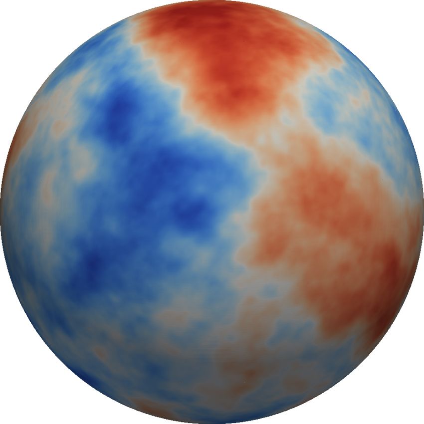
and                                                                  i.e., the MAP point,

                          1        T −1                                            x̄post ≈ xMAP := arg max πpost (x).
        πnoise (e) ∝ exp − (e − ē) Γnoise (e − ē) ,                                                       x
                          2
                                                                     This approximation is exact when the map from parameters
respectively, where x̄prior is the mean of the prior distribution,
                                                                     to observables, f (x), is linear. Finding the MAP point is
ē is the mean of the Gaussian noise, Γprior ∈ Rn×n is the
                                                                     equivalent to minimizing the negative log of the posterior pdf,
covariance matrix for the prior, and Γnoise ∈ Rm×m is the
                                                                     i.e.,
covariance matrix for the noise. Restating Bayes’ theorem with
these Gaussian pdf’s, we find that the statistical solution of the                       x̄post ≈ arg min V (x),                   (2)
                                                                                                        x
inverse problem, πpost (x), is given by
                         1                                          where
        πpost (x) ∝ exp − kx − x̄prior k2Γ−1                                     1                         1
                              2              prior                     V (x) =     ky − f (x) − ēk2Γ−1+ kx − x̄prior k2Γ−1 .      (3)
                              1                                                 2 obs               noise 2             prior
                           − ky obs − f (x) − ēk2Γ−1 ,        (1)
                              2                      noise           Approximating the mean of the posterior distribution by find-
Note that the seemingly simple expression f (x) belies the           ing the MAP point is thus equivalent to solving a regularized
complexity of the underlying computations, which involve:            deterministic inverse problem, where Γ−1   prior plays the role of
                                                                                                          −1
(1) construction of the PDE model for given parameters x;            the regularization operator, and Γnoise is a weighting for the
(2) solution of the governing PDE model to yield the output          data misfit term.
state variables; and (3) extraction of the observables from             Here, we solve the nonlinear least squares optimization
the states at the observation locations in space and time. In        problem (2) with a parallel inexact Newton–conjugate gradient
§VII, we provide expressions for the underlying mathematical         method. The method requires the computation of gradients
operators for our target inverse seismic wave propagation            and Hessian-vector products of V (x) (for which expressions
problem, in which the parameters are wave speeds in the earth,       are provided in §VII in the context of the seismic inverse
the governing PDEs describe acoustic wave propagation, and           problem we target). Rather than provide a detailed description
the observations are of velocity waveforms at seismometer            of the method here, we refer to our earlier work presented
locations on earth’s surface. In general, f (x) is nonlinear, even   at SC2002 [8] and SC2003 [9] on parallel scalability of the
when the forward PDEs are linear in the state variables (as is       method, as well as the recent work [10] that includes additional
the case for the seismic inverse problem), since the model           refinements. The main ingredients of the method are:
parameters couple with the states nonlinearly in the forward            • inexact Hessian matrix-free Gauss-Newton-conjugate
PDEs.                                                                     gradient (CG) minimization;
                                                                                                  −1
   As is clear from the expression (1), despite the choice              • preconditioning by Γprior , carried out by multigrid V-
of Gaussian prior and noise probability distributions, the                cycles on the underlying elliptic operators;
posterior probability distribution need not be Gaussian, due            • Armijo-type backtracking line search globalization;
to the nonlinearity of f (x). The non-Gaussianity of the                • computation of gradients of V (x) and products of Hes-
posterior poses challenges for computing statistics of interest           sians of V (x) with vectors at each CG iteration expressed
for typical large-scale inverse problems, since as mentioned              as solutions of forward and (backward-in-time) adjoint
in §I, πpost is often a surface in high dimensions (millions,             PDEs and their linearizations, all of which inherit the
in our target problem in §VII), and evaluating each point                 parallel scalability properties of the forward PDE solver;
on this surface requires the solution of the forward PDEs               • algorithmic checkpointing to implement the composition
(wave propagation equations with O(109 ) unknowns, in the                 of forward-in-time forward PDE solutions and backward-
target problem). Numerical quadrature to compute the mean                 in-time adjoint PDE solutions to form gradients without
and covariance matrix, for example, is completely out of                  having to store the entire state variable time history; and
the question. The method of choice for computing statistics             • parallel implementation of all components of the method,
is Markov chain Monte Carlo (MCMC), which judiciously                     which are dominated by solution of forward and adjoint-
samples the posterior distribution, so that sample statistics can         PDEs and evaluation of inner product-like quantities to
be computed. But the use of MCMC for large-scale inverse                  compose gradient and Hessian-vector quantities.
problems is still prohibitive for expensive forward problems         What can be said about parallel and algorithmic scalability
and high dimensional parameter spaces, since even for modest         of this method? Because the dominant components of the
numbers of parameters, the number of samples required can be         method can be expressed as solutions or evaluations of PDE-
in the millions. An alternative approach based on linearizing        like systems, parallel scalability—that is, maintaining high
the parameter-to-observable map is discussed next.                   parallel efficiency as the number of cores increases—is assured
                                                                     whenever a scalable solver for the underlying PDEs is avail-
          III. P OSTERIOR MEAN APPROXIMATION                         able (which is the case for our target seismic wave propagation
  The mean of the posterior distribution x̄post can be approx-       problem [11]). The remaining ingredient to obtain overall
imated by finding the point that maximizes the posterior pdf,        scalability is that the method exhibit algorithmic scalability,
that is with increasing problem size. This is indeed the case:               IV. P OSTERIOR COVARIANCE APPROXIMATION
for a wide class of nonlinear inverse problems, the outer
Newton iterations and the inner CG iterations are independent          For many ill-posed inverse problems, the Hessian matrix of
of the mesh size (as is the case for our target inverse wave         the data misfit term in (3), defined as
propagation problem, [10]). This is a consequence of the use                                         def
of a Newton solver, of the compactness of the Hessian of the                                H misfit = AT Γ−1
                                                                                                           noise A,                   (5)
data misfit term (i.e., the first term on the right hand side
of (3), as proven for the inverse wave propagation setting           is a discretization of a compact operator, i.e., its eigenvalues
in [4]), and the choice of prior preconditioning so that the         collapse to zero. This can be understood intuitively, since only
resulting preconditioned Hessian is a compact perturbation of        the modes of the parameter field that strongly influence the
the identity, for which CG exhibits mesh-independent itera-          observations (through the linearized parameter-to-observable
tions. Thus, solving the least squares optimization problem          map A) will be present in the dominant spectrum of (5).
(2) to approximate the mean of the posterior distribution            In many ill-posed inverse problems, observations are sparse
by the method outlined above exhibits both parallel and              compared to the parameter dimensions, and numerous modes
algorithmic—and thus overall—scalability.                            of the parameter field (for example, highly oscillatory ones)
                                                                     will have negligible effect on the observables. The range space
   As stated above, the focus of this paper is not on the com-
                                                                     thus is effectively finite-dimensional even before discretization
putation of the posterior mean x̄post , but on the significantly
                                                                     (and therefore independent of any mesh), and the eigenvalues
more challenging task of characterizing the uncertainty in
                                                                     decay, often rapidly, to zero. In this section, we exploit
the mean via computation of the posterior covariance matrix,
                                                                     this low-rank structure to construct scalable algorithms to
Γpost ∈ Rn×n . Linearizing the parameter-to-observable map at
                                                                     approximate the posterior covariance operator.
the MAP point gives
                                                                        Rearranging the expression for Γpost in (4) to factor out
                                                                       1/2
                                                                     Γprior gives
              f (x) ≈ A(x − xMAP ) + f (xMAP ),
                                                                                                                    −1
                                                                                  1/2    1/2               1/2            1/2
                                                                         Γpost = Γprior Γprior AT Γ−1
                                                                                                   noise AΓprior + I     Γprior .     (6)
where A ∈ Rm×n is the Jacobian matrix of f (x) evaluated
at xMAP . Manipulation of (1) shows that Γpost is given by the       This factorization exposes the prior-preconditioned Hessian of
inverse of the Hessian matrix of the function V (x) in (3), i.e.,    the data misfit,
                                                                                              def    1/2               1/2
                                          −1                                        H̃ misfit = Γprior AT Γ−1
                                                                                                             noise AΓprior .          (7)
              Γpost = AT Γ−1
                          noise A + Γ−1
                                     prior     .              (4)
                                                                     In the next section we present a randomized algorithm to
In summary, under the assumptions of this section (additive          construct a low rank approximation of this matrix at a cost (in
Gaussian noise, Gaussian prior, and linearized parameter-to-         PDE solves) that is independent of the parameter dimension
observable map), solution of the Bayesian inverse problem            (compared to n PDE solves to construct the full matrix). In this
is reduced to the characterization of the (Gaussian) posterior       section, we assume only that such a low rank construction is
distribution N (x̄MAP , Γpost ), where Γpost is the inverse of the   possible. Let λi and v i be the eigenvalues and eigenvectors of
Hessian of V (x) at xMAP .                                           H̃ misfit . Let Λ = diag(λi ) ∈ Rn×n be the diagonal matrix
                                                                     of its eigenvalues, and define as V ∈ Rn×n the matrix
   The primary difficulty here is that the large parameter
                                                                     whose columns are the eigenvectors v i of H̃ misfit . Then replace
dimension n prevents any representation of the posterior
                                                                     H̃ misfit by its spectral decomposition:
covariance Γpost as a dense operator. In particular, the Jacobian
of the parameter-to-observable map, A, is formally a dense
                                                                             1/2               1/2
                                                                                                           −1
matrix, and requires n forward PDE solves to construct. This                Γprior AT Γ−1
                                                                                       noise AΓprior + I         = (V ΛV T + I)−1 .   (8)
is intractable when n is large and the PDEs are expensive,
as in our case. However, a key feature of the operator A is          When the eigenvalues of H̃ misfit decay rapidly, we can extract
that its action on a (parameter field-like) vector can be formed     a low-rank approximation of H̃ misfit by retaining only the r
by solving a (linearized) forward PDE problem; similarly, the        largest eigenvalues and corresponding eigenvectors,
action of its transpose AT on a (observation-like) vector can
                                                                                      1/2                  1/2
be formed by solving a (linearized) adjoint PDE. Explicit                           Γprior AT Γ−1                       T
                                                                                               noise AΓprior ≈ V r Λr V r .
expressions for these operations will be given for our specific
target inverse problem in §VII. In the next two sections, we         Here V r ∈ Rn×r contains only the r eigenvectors of H̃ misfit
present algorithms that exploit this property, as well as the        that correspond to the r largest eigenvalues, which are as-
spectral decay of the data misfit Hessian, to approximate the        sembled in the diagonal matrix Λr = diag(λi ) ∈ Rr×r .
posterior covariance matrix with controlled accuracy at a cost       To obtain the posterior covariance matrix, we employ the
that is independent of the parameter dimension.                      Sherman-Morrison-Woodbury formula to perform the inverse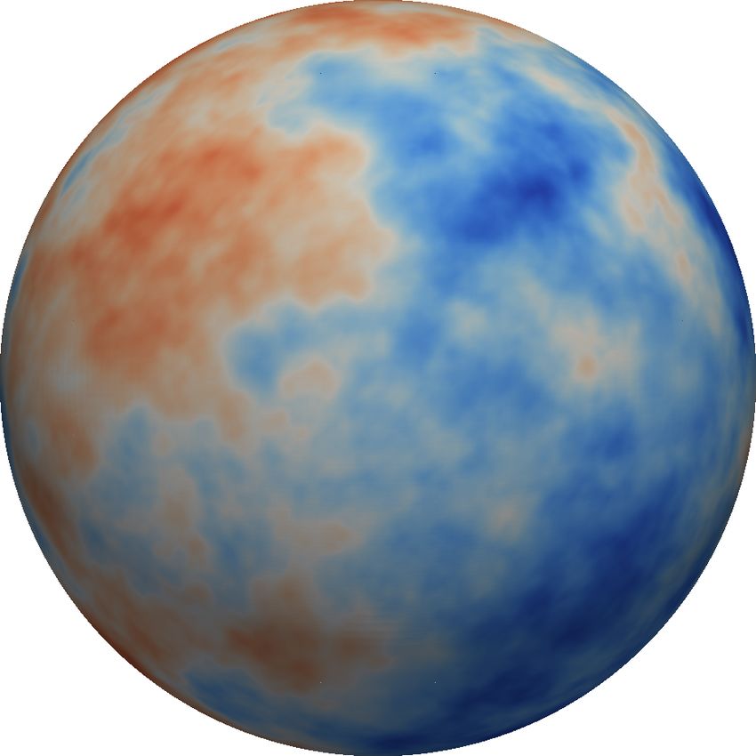
7
                                                                                                 10
in (6),                                                                                                                                           40,842 parameters
                                                                                                                                                  67,770 parameters
                                                                                                  6                                               431,749 parameters
                                   −1                                                          10
        1/2               1/2
       Γprior AT Γ−1
                  noise AΓprior + I     =                                                         5
                                                                                                 10
                                                n
                                                            !
                                                X     λi
                    I − V r D r V Tr + O                        ,                                 4
                                                                                                 10
                                                    λ  +1

                                                                                    eigenvalue
                                               i=r+1 i                                            3
                                                                                                 10

            def
where D r = diag(λi /(λi + 1)) ∈ Rr×r . The last term in                                          2
                                                                                                 10

the expression above shows the error due to truncation in
                                                                                                  1
                                                                                                 10
terms of the discarded eigenvalues; this provides a criterion
for truncating the spectrum, namely r is chosen such that λr is                                   0
                                                                                                 10

small relative to 1. With this low-rank approximation, the final
                                                                                                  −1

expression for the approximate posterior covariance follows                                      10
                                                                                                       0       100   200    300    400      500        600         700
                                                                                                                              number
from (6),
                                 1/2                1/2                   Fig. 1.    Log-linear plot of the spectrum of prior-preconditioned
            Γpost ≈ Γprior − Γprior V r D r V Tr Γprior .           (9)   data misfit Hessian (H̃ misfit ) for three successively finer parameter
                                                                          meshes of an inverse wave propagation problem [7]. The spectra lie
Note that (9) expresses the posterior uncertainty (in the form            on top of each other, indicating mesh independence (and therefore
of a covariance matrix) as the prior uncertainty, less any                parameter-dimension independence) of the low rank approximation.
information gained from the data, filtered through the prior.             The eigenvalues are truncated when they are small relative to 1, which
                                                                          in this case results in retaining between 0.2 and 2% of the spectrum.
V. A RANDOMIZED ALGORITHM FOR LOW- RANK H ESSIAN
                        APPROXIMATION
                                                                          the former, in the typical case when the PDE model governing
   We now address the construction of the low rank approx-
                                                                          the inverse problem is large scale.
imation of H̃ misfit that was invoked in the previous section.
                                                                             Let Q be an orthonormal basis for Y , which approximates
As argued above, the data inform only a limited number
                                                                          the range space of H̃ misfit . Following the “single-pass” ap-
of modes of the parameter field, resulting in a data misfit
                                                                          proach of [13], we compute the approximation to H̃ misfit in
Hessian matrix that admits a low rank representation. This
                                                                          the basis Q:
is observed numerically (see Figure 1) and has recently been
proven theoretically in several settings [4], [12]. Moreover,                                                def
                                                                                                           B = (QT Y )(QT R)−1 ≈ QT H̃ misfit Q.                         (10)
preconditioning with the prior operator as in (7) further filters
out modes of the parameter space that are already well-                   Here B, QT Y , and (QT R)−1 are all matrices of dimension
determined from prior knowledge (i.e., a smoothing prior such             r, which is much smaller than n, and thus we are able
as the one we employ here assigns low probability to highly               to decompose the symmetric matrix B as ZΛZ T using
oscillatory modes.)                                                       dense linear algebra. The dominant vectors of H̃ misfit are then
   We exploit this structure to construct a low rank approxima-           returned as V = QZ, with eigenvalues on the diagonal of Λ.
tion of H̃ misfit using randomized algorithms for approximate             Thus, we find the desired decomposition
matrix decomposition [13], [14]. Their performance is compa-
rable to Krylov methods (such as Lanczos) we employed pre-                                                           H̃ misfit ≈ V ΛV T .                                (11)
viously [5], [15]. However, they have a significant edge over
                                                                          Finally, randomized methods also provide an estimate of the
these deterministic methods for large-scale problems, since
                                                                          spectral norm of I −QQT H̃ misfit , which bounds the error that
the required Hessian matrix-vector products are independent
                                                                          we make in our low rank approximation. To be precise, the
of each other, providing asynchronousity and fault tolerance.
                                                                          bound derived in [13] is
Before discussing these advantages, let us summarize the
algorithm.
                                                                                                      r
                                                                                                          2
   To approximate the spectral decomposition of H̃ misfit ∈                 (I − QQT )H̃ misfit ≤ α          max (I − QQT )Aω (i) ,
                                                                                                          π i=1,...,r
Rn×n , we generate a random matrix R ∈ Rn×r (r is                                                                                    (12)
of the order of the numerical rank of H̃ misfit , so in our               attained with probability of at least 1 − α−r , where ω (i) are
case r  n) with i.i.d. Gaussian entries, and compute the                 vectors with i.i.d. standard normal entries.
product Y = H̃ misfit R. Since each column vector in R is an                 To summarize, the construction of a low-rank approximation
independent random vector, the computation of Y decouples                 of H̃ misfit is dominated by its application to random vectors,
into r separate matrix-vector product with H̃ misfit . As can be          which entails a pair of forward/adjoint PDE solves. The inde-
seen from (7), each matrix-vector product requires a pair of              pendence of these matrix-vector products from each other is
forward/adjoint PDE solves (to form actions of A and AT on                of particular importance for problems in which the parameter-
vectors), as well as a pair of elliptic operator solves (to form          to-observable map f (x) has to be computed on large parallel
             1/2
actions of Γprior on vectors). The latter are much cheaper than           supercomputers for the following reasons: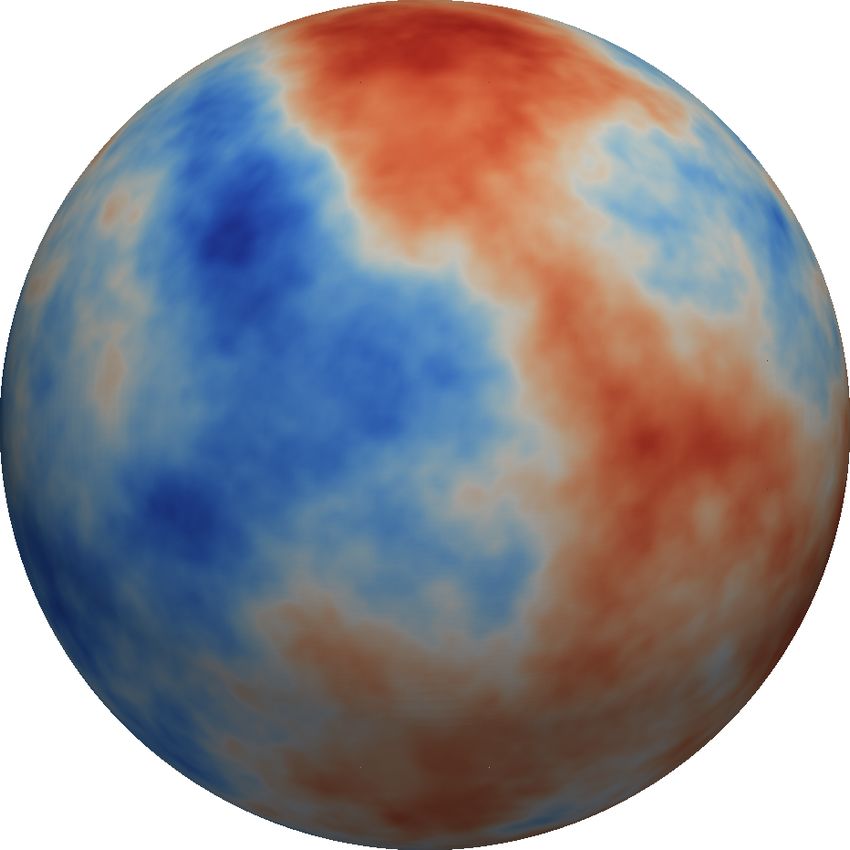
•   Cache and memory efficiency: For parameter-to-                  rate can be shown to be exponential. That is, the data misfit
      observable maps that involve the solution of a PDE, the         Hessian can be approximated well with a handful of its
      application of the Hessian to multiple vectors requires         dominant eigenvectors and eigenvalues. In conclusion, a low-
      the solution of (linearized) forward/adjoint PDEs for           rank approximation of H̃ misfit can be made that does not
      multiple right-hand sides. Amortizing data movement             depend on the parameter dimension, and depends only on the
      over the multiple right-hand sides results in significantly     information content of the data, filtered through the prior.
      greater memory and cache efficiency than can be obtained           Once the r eigenpairs defining the low rank approximation
      with sequential right-hand sides, as required by classical      have been computed, estimates of uncertainty can be computed
      Krylov methods.                                                 by interrogating Γpost in (9) at a cost of just r inner products
  •   Fault-tolerance: the construction of the low-rank matrix        (which are negligible) plus elliptic solves representing the
                                                                                                                 1/2
      approximation is done as a post-processing step when a          action of the square root of the prior Γprior on a vector (here
      sufficient number of matrix-vector products is available.       carried out with algebraic multigrid and therefore scalable).
      The asynchronous nature of the matrix-vector products           For example, samples can be drawn from the Gaussian de-
      provides greater fault tolerance (for example, the low rank     fined with a covariance Γpost , a row/column of Γpost can be
      approximation in §VII was computed using 10 different           computed, and the action of Γpost in a given direction can be
      jobs with different run times and core counts ranging           formed, all at cost that is O(rn) for the inner products in
      from 32K to 108K.                                               addition to the O(n) cost of the multigrid solve. Moreover,
                                                                      the posterior variance field, i.e., the diagonal of Γpost , can be
           VI. S CALABILITY OF THE UQ METHOD                          found with O(rn) linear algebra plus O(r) multigrid solves.
   We now discuss the overall scalability of our UQ method               In summary, we have a method for estimating the posterior
to high-dimensional parameter spaces. First, we summarize             covariance—and thus the uncertainty in the solution of the
the scalability of the construction of the low-rank-based             linearized inverse problem—that requires a constant number
approximate posterior covariance matrix in (9). As stated             of PDE solves, dependent only on the information content of
before, the linearized parameter-to-observable map A cannot           the data filtered through the prior (i.e., r), but independent
be constructed explicitly, since it requires n linearized forward     of the number of parameters (n), the number of observations
PDE solves. However, its action on a vector can be computed           (m), and the number of state variables. Moreover, since the
by solving a single linearized forward PDE, regardless of the         dominant cost of the posterior covariance construction is that
number of parameters n and observations m. Similarly, the             of solving forward and adjoint-like PDEs, parallel scalability
action of AT on a vector can be computed by solving a                 of the overall uncertainty quantification method follows when
linearized adjoint PDE. Moreover, the prior is usually much           the forward PDE solver is scalable (this will be demonstrated
cheaper to apply than the forward or adjoint PDE solution (in         for the case of our seismic wave propagation solver in the next
our context, it is a single elliptic solve). Therefore, the cost of   section).
applying H̃ misfit to a vector—and thus the per iteration cost of
the randomized algorithm of §V—is dominated by the solution               VII. A PPLICATION TO GLOBAL SEISMIC INVERSION
of a pair of linearized forward and adjoint PDEs (explicit               In recent years, the methodology for scalable parallel so-
expressions for this matrix-vector product will be given for          lution of forward seismic wave propagation problems on
the target problem of inverse wave propagation in §VII).              supercomputers by spectral element [17], [18], finite differ-
   The remaining component to establish scalability of the low-       ence [19], finite element [9], and discontinuous Galerkin [20]
rank approximation of H̃ misfit is independence of the rank           methods has matured. This motivates our present interest in the
r—and therefore the number of matrix-vector products, and             seismic inverse problem of determining an earth model from
hence PDE solves—from the parameter dimension n. This                 surface observations of seismic waveforms; indeed, we are
is the case when H misfit in (5) is a (discretization of a)           interested not just in the solution of this inverse problem, but
compact operator, and when preconditioning by Γprior does             in quantifying the uncertainties in its solution using the method
not destroy the spectral decay. This situation is typical for         proposed in this paper. In previous sections, our method and
many ill-posed inverse problems, in which the prior is either         underlying algorithms were presented for generic prior and
neutral or of smoothing type (here, we employ a prior that is         likelihood functions. §VII-A provides explicit expressions for
the inverse of an elliptic operator). Compactness of the data         these functions (in infinite dimensions) for the specific seismic
misfit Hessian H misfit for inverse wave propagation problems         inverse problem we address, along with explicit expressions
has long been observed (e.g., [16]). Recently, we have proven         for gradient and Hessian-vector products, which are needed
compactness for the inverse wave propagation problem for              for computing the mean and covariance estimates. The latter
both continuous and pointwise observation operators for both          expressions involve solutions of forward and adjoint wave
shape and medium scattering [4], [12]. Specifically, we have          propagation PDEs and their linearizations. §VII-B gives an
shown that the data misfit Hessian is a compact operator. We          overview of the forward wave equation solver and provides
also quantify the decay of data misfit Hessian eigenvalues in         near-full system strong scalability results on the Jaguar super-
terms of the smoothness of the medium, i.e., the smoother             computer at ORNL. §VII-C describes the setup of the seismic
it is, the faster the decay rate. Under some conditions, the          inverse problem: the configuration of sources and receivers, the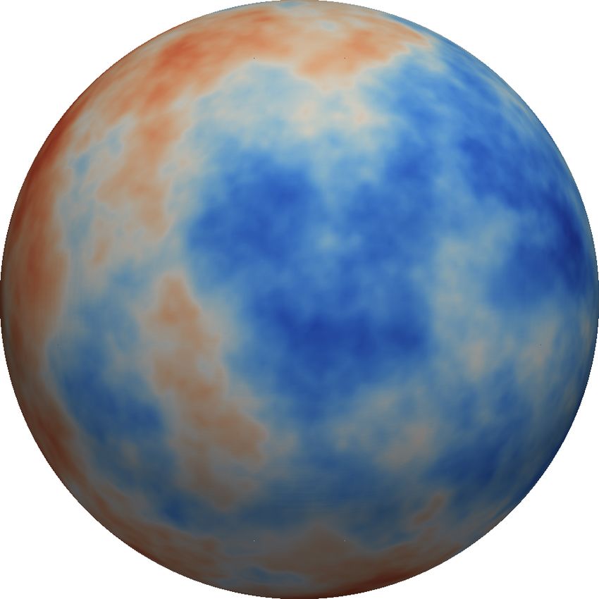
generation of synthetic seismogram observations, the choice                Similarly, the action of the Hessian operator in the direction
of prior and noise covariances, the parametrization of wave             c̃ at a point c is given by
speed, and the mesh generation. §VII-C presents results on                            Z T
quantifying uncertainties in the solution of a linearized global        H(c)c̃ := 2ρ ce(∇ · w̃)+cẽ(∇ · w)+c̃e(∇ · w) dt + Γ−1      prior c̃,
seismic inverse problem characterized by one million uncertain                           0

parameters. This is the largest—in fact the first—solution of           where ṽ and ẽ satisfy the incremental forward wave propaga-
which we are aware of a statistical inverse problem whose               tion equations
forward solver has required a supercomputer, made possible
                                                                                  ρv t − ∇(ρc2 ẽ) = ∇(2ρcc̃e) in Ω × (0, T ),
because of the parameter-dimension-independent scaling of
our method.                                                                             et − ∇ · ṽ = 0                in Ω × (0, T ),
                                                                                         ρṽ = 0, ẽ = 0               in Ω × {t = 0} ,
A. Posterior and its derivatives                                                                    ẽ = 0             on Γ × (0, T ).
   In this section we give explicit expressions for V (x), the
                                                                        On the other hand, w̃ and d˜ satisfy the incremental adjoint
negative log of the posterior pdf for the seismic inverse
                                                                        wave propagation equations
problem we target, along with expressions for its gradient and
Hessian-vector product. The expressions are written in strong,                       ˜ = −∇(2c̃cρd) − B ∗ Γ−1 Bṽ in Ω × (0, T ),
                                                                        −ρwt + ∇(c2 ρd)                    noise
infinite-dimensional form, for clarity. The inversion parameter               −dt + ∇ · w̃ = 0                                        in Ω × (0, T ),
is taken as c = c(x), the local acoustic wave speed of the
medium. We can write the negative log posterior as                             ρw̃ = 0, d˜ = 0                                        in Ω × {t = T } ,
                                                                                             d˜ = 0                                   on Γ × (0, T ).
               1                   2            1         2
     V(c) :=     Bv(c) − v obs     Γ−1
                                            +     kc − c̄kΓ−1 ,
               2                    noise       2           prior       The incremental forward and incremental adjoint wave equa-
where the data misfit (the first term) is a finite dimensional          tions are seen to be linearized versions of their forward and
norm due to the pointwise observations in time and space,               adjoint counterparts, and thus differ only in the source terms.1
and the prior term (the second term) is an infinite dimensional            Thus, we see that computation of gradients (as needed in the
norm, with the elliptic prior operator Γ−1                              posterior mean approximation) and Hessian actions on vectors
                                             prior taken as an
anisotropic biharmonic. The wave propagation variables—the              (as needed in the posterior covariance approximation) amount
velocity vector v and the trace of the strain tensor e (i.e., the       to solution of a pair of forward/adjoint wave equations each.
dilation) depend on c through the solution of the forward wave          B. Wave propagation solver and its strong scalability
propagation equations (written in first-order form):
                                                                           The forward wave equation, and its three variants (adjoint,
            ρv t − ∇(ρc2 e) = g in Ω × (0, T ),                         incremental forward, incremental adjoint) described in the
                                                                        previous section, are solved using a high-order discontinuous
                 et − ∇ · v = 0 in Ω × (0, T ),
                                                                        Galerkin (dG) method. Details on the forward solver are
                  ρv = 0, e = 0 in Ω × {t = 0},                         provided in [11]; here we summarize the salient features:
                           e = 0 on ∂Ω × (0, T ).                          • discretization that supports h-nonconforming hexahedral
                                                                             elements on a 2:1 balanced forest-of-octrees mesh;
Here, ρ and g are known density and seismic source, v obs are              • an element basis that is a tensor product of Lagrange
observations at receivers, B is an observation operator, and                 polynomials of arbitrarily high degree based on the
Γprior and Γnoise are the prior and noise covariance operators.              Legendre-Gauss-Lobatto (LGL) nodes;
   The adjoint approach allows us to write the gradient at a               • LGL numerical quadrature, which produces a diagonal
given point c in parameter space as                                          mass matrix;
                      Z T                                                  • solution of the Riemann problem at material interfaces
         G(c) := 2ρc      e(∇ · w) dt + Γ−1prior (c − c̄),                   (elastic-elastic, elastic-acoustic, acoustic-acoustic);
                       0
                                                                           • mortar-based implementation of flux on 2:1 nonconform-
where the adjoint velocity w and adjoint strain dilation d                   ing faces;
satisfy the adjoint wave propagation equations                             • time integration by classical four-stage fourth-order
                                                                             Runge Kutta;
−ρwt + ∇(c2 ρd) = −B ∗ Γ−1
                        noise (Bv − v
                                      obs
                                          ) in Ω × (0, T ),                • guaranteed consistency, semi-discrete stability, and opti-
     −dt + ∇ · w = 0                                in Ω × (0, T ),          mal order convergence for non-conforming meshes [21].
       ρw = 0, d = 0                                in Ω × {t = T } ,      1 The infinite dimensional expressions for the gradient and Hessian action
                 d=0                                on Γ × (0, T ).     given above are actually not consistent with the discrete gradient and Hessian-
                                                                        vector product obtained by first discretizing the negative log posterior and
The adjoint wave equations are reversed in time and have the            wave equation and then differentiating with respect to parameters. Additional
                                                                        jump terms at element interfaces due to the dG discretization appear; in our
data misfit as source term, but otherwise resemble the forward          implementation, we include these terms to insure consistency with discrete
wave equations.                                                         counterparts.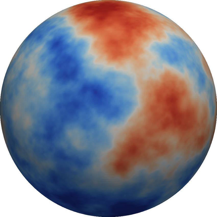
TABLE I
   To model global seismic wave propagation, we model the                          S TRONG SCALING OF THE FORWARD SOLVER
earth as a sphere with a radius of 6,371 km, where the speed                   #cores     time [ms]      elem/core      efficiency [%]
of acoustic (pressure) waves varies throughout the domain.                       256       1630.80          4712             100.0
To generate the finite element mesh, we decompose the earth                      512        832.46          2356              98.0
into 13 warped cubes. The inner core comprises one central                      1024        411.54          1178              99.1
cube, surrounded by two layers of six additional cubes. Each                    8192        61.69           148               82.6
                                                                               65536        11.79            19               54.0
cube is the root of an adaptive octree, which can be arbitrarily              131072         7.09            10               44.9
refined, thus creating a mesh of curved hexahedral elements.                  262144         4.07             5               39.2
The mesh is aligned to the interface between the outer core and                 1024       5423.86         15817             100.0
the mantle, and several weaker discontinuities between layers,                  4096       1407.81          3955              96.3
and refined locally to resolve varying seismic wavelengths up                   8192        712.91          1978              95.1
to a target frequency. The wave speed c(x) is approximated                     16384        350.43           989              96.7
                                                                               32768        211.86           495              80.0
with piecewise trilinear finite elements, and the wave equation                65536        115.37           248              73.5
variables (velocity and strain) are discretized using high-order              131072        57.27           124               74.0
(spectral) discontinuous Galerkin finite elements on the same                 262144        29.69            62               71.4
hexahedral mesh. For the distributed storage and adaptation of      Strong scaling results on ORNL’s Jaguar XK6 system for global seismic wave
both the parameter and wave propagation meshes, we use our          propagation solutions for two problem sizes. We report the time per time step
p4est library of fast forest-of-octree algorithms for scalable      in milliseconds on meshes with 1,206,050 (upper table) and 16,195,864 (lower
                                                                    table) 3rd order discontinuous Galerkin finite elements, corresponding to 694
adaptive mesh refinement, which have been shown to scale to         million and 9.3 billion spatial degrees of freedom, respectively. The elem/core
over 220,000 CPU cores and impose minimal computational             column reports the maximum number of elements owned by any core. For
overhead [20], [22]. The time spent in meshing is insignificant     strong scaling from 256 to 262,144 cores, the parallel efficiency is still as
                                                                    high as 39% for the small problem. For the larger problem and a 256-fold
relative to that of numerical solution of the wave equation.        increase in problem size, we find a parallel efficiency of 71%. At 262,144
                                                                    cores, each core owns just 4 or 5 elements for the small problem, and 61 or
   The central difficulty of UQ is its need for repeated solution   62 elements for the larger problem. The larger run sustains a double precision
                                                                    floating point rate of 111 teraflops per second (based on performance counters
of the governing PDE model, in our case the wave propagation        from the PAPI library [23].
equations. Conventional sampling methods will take millions
of wave propagation solutions (realistically, much more) to
explore the posterior distribution for the million-parameter
problem we solve in this section. For the frequencies we
target, a single wave propagation solve takes a minute on
64K Jaguar cores; conventional sampling methods are thus
out of the question. The low-rank Hessian-based method we
have presented here, which captures and exploits the local
structure of the posterior in the directions informed by the
data by computing curvature information based on additional
wave equations (adjoint and incremental forward and adjoint),
reduces the number of wave propagation solutions by orders          Fig. 2. (Coarser version of) mesh used for the wave propagation simulation
of magnitude. Still, thousands of wave equation solves are          and “true” pressure wave speed c in km/s. Left: section through earth model.
needed, and we must use all available computing resources. As       Right: surface at depth of 222 km showing lateral variations of up to 7%.
                                                                    Wave propagation mesh is tailored to the local seismic wave lengths.
a result, we insist on excellent strong scalability of our wave
equation solver to achieve acceptable time-to-solution. Taken
together, the high-order discretization, discontinuous elements,
explicit RK scheme, and space filling curve partitioning un-        C. Inverse problem solution and its uncertainty
derlying our forest-of-octree mesh data structure should yield         This section presents solution of the statistical inverse
excellent scalability; indeed, we have shown near ideal parallel    problem. First we define the inverse problem setup. Both
efficiency in weak scaling on up to 220,000 cores of the Jaguar     the prior mean and the initial guess for the iterative so-
system at ORNL [11]. Here, we investigate the extreme limits        lution of the nonlinear least squares optimization problem
of strong scaling to determine how fine a granularity one can       (2) (to find the MAP point) are derived from the radially
employ in the repeated wave solutions. Table I shows that our       symmetric preliminary reference earth model (PREM) [24],
wave equation solver exhibits excellent strong scaling over         which dates to 1981. We take the “true” earth to be given
a wide range of core counts. These results are significant,         by the more recent S20RTS velocity model (converted from
since we are using just third-order elements (higher order          shear to acoustic wave speed anomaly) [25], which superposes
creates more work per element, relative to data movement).          lateral wave speed variations on PREM, as seen in Figure 2.
For the large problem, for example we maintain 71% parallel         Synthetic observations are generated from solution of the wave
efficiency in strong scaling from 1024 to 262,144 cores. The        equation for an S20RTS earth model, with seismic sources
largest core count problem has just 62 elements per core.           at the North pole and at 90◦ intervals along the equator,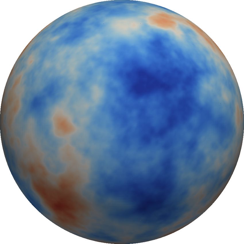
Fig. 4. Comparison of MAP of posterior pdf (left) with the “true” earth
                                                                            model (right) at a depth of 67 km. Source locations are indicated with black
Fig. 3. Location of five simultaneous seismic sources (black spheres; two   spheres and seismic receiver stations are indicated by white spheres.
in back not visible) and 100 receivers (white spheres).

                                                                                                       6
                                                                                                      10

all of them at a depth of 10 km. All five point sources are                                            5
                                                                                                      10
taken to occur simultaneously. A total of 100 receivers in the
Northern and Eastern hemispheres are distributed along zonal                                           4
                                                                                                      10

lines at 10◦ spacing. The source and receiver configuration                                            3
                                                                                                      10

                                                                                         eigenvalue
is illustrated in Figure 3. The observations consist of the first
                                                                                                       2

61 Fourier coefficients of the Fourier-transformed seismogram                                         10

(time history of ground motion) at each receiver location. The                                         1
                                                                                                      10

noise distribution for these data is taken as i.i.d. Gaussian with                                     0
                                                                                                      10

mean zero and a standard deviation of 9.34 × 10⁻³ .
                                                                                                       −1

   We use a 3rd-order discontinuous finite elements mesh to                                           10
                                                                                                            0   50   100   150   200     250
                                                                                                                                       number
                                                                                                                                                300   350   400   450   500

resolve seismic wavelengths corresponding to a source with
maximum frequency of 0.07 Hz. This requires a mesh with                     Fig. 5. Logarithmic plot of the spectrum of prior-preconditioned data misfit
                                                                            Hessian.
1,093,784 elements, which leads to 630 million wave propa-
gation spatial unknowns (velocity and strain) for the forward
problem, and 1,067,050 unknown wave speed parameters for
the statistical inverse problem. The observation time window
for the inverse problem is 1,000 seconds, which leads to 2400                  We approximate the covariance matrix at the MAP point
discrete time steps. This simulation time is sufficient for the             via a low-rank representation employing 488 products of the
waves to travel about two-thirds of the earth’s diameter. A                 Hessian matrix with random vectors. The effective problem
single wave solve takes about one minute on 64K Jaguar                      dimension is thus reduced from 1.07 million to 488, a factor of
cores. As discussed in §VII-A, two wave solves are needed                   over 2000 reduction. Figure 5 depicts the first 488 eigenvalues
in each gradient or Hessian-vector computation. However,                    of the million-dimensional parameter field, indicating the rapid
since these expressions combine wave equation solutions in                  decay in information content of the data, a fact that we exploit
opposite time direction, the work-optimal choice of solving                 to make the UQ problem tractable.
two wave equations requires storage of the entire time history,                The reduction in the variance between prior and posterior
which is prohibitive. Instead, we use algorithmic checkpoint-               due to the information (about the earth model) content of
ing methods, which cut the necessary storage but increases                  the data—i.e., the diagonal of the second term in (9), the
the number of wave propagation solutions to five per Hessian-               expression for the posterior covariance—is shown in Figure
vector product (two forward, two incremental forward, and                   7. We observe that in the region where sensors are placed (the
one adjoint solve) [10]. Thus, a single Hessian-vector product              visible portion of the Northern hemisphere), we get a large
takes about 5 minutes on 65K Jaguar cores.                                  reduction in variance due to the data. In regions where there
   The posterior mean is approximated by solving the nonlin-                are no sensors, the reduction in variance is substantially less.
ear least squares optimization problem (2) to find the MAP                  Additionally, Figure 8 displays the variance reduction on a
point, using the inexact Gauss Newton-CG method described                   slice through the equator of the earth, and we again see that
in §II, initialized with the prior mean (the PREM model),                   the largest variance reduction (depicted in red) is achieved
and terminated after 3 orders of magnitude reduction in the                 near the surface where the sensors are located, although some
gradient, which was achieved after a total of 320 CG iterations             reduction is also achieved well into the earth’s mantle. Finally,
(summed across Newton iterations). A comparison of the                      Figure 6 shows samples from the prior and the posterior
approximate mean with the “true” earth model (S20RTS) is                    pdf; the difference between the two sets of samples reflects
displayed in Figure 4. The MAP solution is seen to resemble                 the information gained from the data in solving the inverse
the “true” parameter field well in the Northern hemisphere,                 problem. Note the regions of large variability in the posterior
which has good receiver coverage.                                           samples, which reflect the absence of receivers.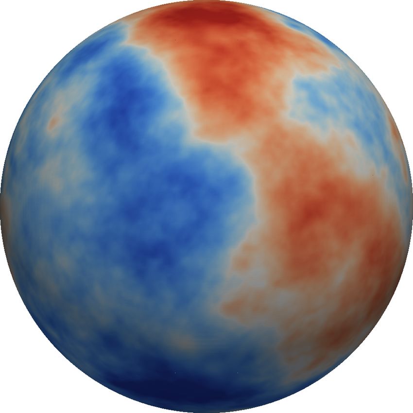
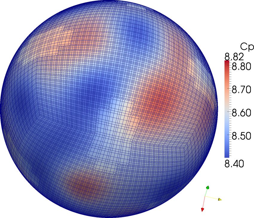
Fig. 6. Samples from the prior (top row) and posterior (bottom row) distributions. The difference between the prior and posterior samples reflects the
information (about the earth model) learned from the data. The large scale features of the posterior samples consistently resemble the posterior mean (right).
The fine scale features however are not expected to be influenced by the data, and qualitatively resemble the fine scale features of the prior samples. Note the
small variability across samples in the Northern hemisphere—reflecting the receiver coverage there—while the Southern hemisphere exhibits large variability
in the inferred model, reflecting that uncertainty due to the lack of receivers.

                                                                                     PDEs, as in our target problem of global seismic inversion.
                                                                                        We have introduced a method that exploits the local struc-
                                                                                     ture of the posterior pdf—namely the Hessian matrix of the
                                                                                     negative log posterior, which represents the local covariance—
                                                                                     to overcome the curse of dimensionality associated with sam-
            Γpost        ≈         Γprior   −   Γ
                                                 1/2       T 1/2
                                                      V D V Γ
                                                                                     pling high-dimensional distributions. Unfortunately, straight-
                                                 prior r r r prior
                                                                                     forward computation of the dense Hessian is prohibitive,
Fig. 7. The left image depicts the pointwise posterior variance field, which is      requiring as many forward-like solves as there are uncertain
represented as the difference between the original prior variance field (middle),
and the reduction in variance due to data (right; see also Figure 8). All variance   parameters. However, the data are typically informative about
fields are displayed at a depth of 67km.                                             a low dimensional subspace of the parameter space—that is,
                                                                                     the Hessian is sparse with respect to some basis. We have
                                                                                     exploited this fact to construct a low rank approximation of the
                                                                                     Hessian and its inverse using a matrix-free parallel randomized
                                                                                     subspace-detecting algorithm. Overall, our method requires
                                                                                     a dimension-independent number of forward PDE solves to
                                                                                     approximate the local covariance. Uncertainty quantification
                                                                                     for the inverse problem thus reduces to solving a fixed number
                                                                                     of forward and adjoint PDEs (which resemble the original
                                                                                     forward problem), independent of the problem dimension. The
                                                                                     entire process is thus scalable with respect to the forward
                                                                                     problem dimension, uncertain parameter dimension, observa-
Fig. 8. Data-induced reduction in variance inside the earth. The reduction
is shown on a slice through the equator, as well as on isosurfaces in the            tional data dimension, and number of processor cores. We
left hemisphere (compare with Figure 7, which shows reduction on earth’s             applied this method to the Bayesian solution of an inverse
surface). As can be seen, the reduction in variance is greatest on the surface.      problem in 3D global seismic wave propagation with one
                                                                                     million inversion parameters, for which we observe 3 orders
                                                                                     of magnitude dimension reduction, which makes UQ tractable.
                          VIII. C ONCLUSIONS                                         This is by far the largest UQ problem that has been solved with
                                                                                     such a complex governing PDE model.
   We have addressed UQ for large-scale inverse problems. We
adopt the Bayesian inference framework: given observational
                                                                                                       IX. ACKNOWLEDGMENTS
data and their uncertainty, the governing forward problem and
its uncertainty, and a prior probability distribution describing                       Support for this work was provided by: the U.S. Air Force
uncertainty in the parameters, find the posterior probability                        Office of Scientific Research (AFOSR) Computational Math-
distribution over the parameters. The posterior pdf is a surface                     ematics program under award number FA9550-09-1-0608; the
in high dimensions, and the standard approach is to sample                           U.S. Department of Energy Office of Science (DOE-SC),
it via a Markov-chain Monte Carlo (MCMC) method and                                  Advanced Scientific Computing Research (ASCR), Scientific
then compute statistics of the samples. However, the use of                          Discovery through Advanced Computing (SciDAC) program,
conventional MCMC methods becomes intractable for high                               under award numbers DE-FC02-11ER26052 and DE-FG02-
dimensional parameter spaces and expensive-to-solve forward                          09ER25914, and the Multiscale Mathematics and Optimization
for Complex Systems program under award number DE-FG02- [16] D. Colton and R. Kress, Inverse Acoustic and Electromagnetic Scat-
08ER25860; the U.S. DOE National Nuclear Security Admin- tering, 2nd ed., ser. Applied Mathematical Sciences, Vol. 93. Berlin,
Heidelberg, New-York, Tokyo: Springer-Verlag, 1998.
istration, Predictive Simulation Academic Alliance Program [17] D. Komatitsch, S. Tsuboi, C. Ji, and J. Tromp, “A 14.6 billion degrees
(PSAAP), under award number DE-FC52-08NA28615; and of freedom, 5 teraflops, 2.5 terabyte earthquake simulation on the
the U.S. National Science Foundation (NSF) Cyber-enabled Earth Simulator,” in SC03: Proceedings of the International Conference
for High Performance Computing, Networking, Storage, and Analysis.
Discovery and Innovation (CDI) program under awards CMS- ACM/IEEE, 2003.
1028889 and OPP-0941678, and the Collaborations in Math- [18] L. Carrington, D. Komatitsch, M. Laurenzano, M. M. Tikir, D. Michéa,
ematical Geosciences (CMG) program under award DMS- N. L. Goff, A. Snavely, and J. Tromp, “High-frequency simulations
of global seismic wave propagation using SPECFEM3D GLOBE on
0724746. Computing time on the Cray XK6 supercomputer 62K processors,” in SC08: Proceedings of the International Conference
(Jaguar) was provided by the Oak Ridge Leadership Com- for High Performance Computing, Networking, Storage, and Analysis.
puting Facility at Oak Ridge National Laboratory, which ACM/IEEE, 2008.
[19] Y. Cui, K. B. Olsen, T. H. Jordan, K. Lee, J. Zhou, P. Small,
is supported by the Office of Science of the Department D. Roten, G. Ely, D. K. Panda, A. Chourasia, J. Levesque, S. M.
of Energy under Contract DE-AC05-00OR22725. Computing Day, and P. Maechling, “Scalable earthquake simulation on petascale
time on the Texas Advanced Computing Center’s Lonestar 4 supercomputers,” in SC10: Proceedings of the International Conference
for High Performance Computing, Networking, Storage, and Analysis.
supercomputer was provided by an allocation from TACC. ACM/IEEE, 2010.
[20] C. Burstedde, O. Ghattas, M. Gurnis, T. Isaac, G. Stadler, T. Warburton,
R EFERENCES and L. C. Wilcox, “Extreme-scale AMR,” in SC10: Proceedings of the
[1] J. T. Oden, R. M. Moser, and O. Ghattas, “Computer predictions with International Conference for High Performance Computing, Networking,
quantified uncertainty, Parts I & II,” SIAM News, vol. 43, no. 9&10, Storage and Analysis. ACM/IEEE, 2010, Gordon Bell Prize finalist.
2010. [21] T. Bui-Thanh and O. Ghattas, “Analysis of an hp-non-conforming
[2] J. Kaipio and E. Somersalo, Statistical and Computational Inverse discontinuous Galerkin spectral element method for wave propagation,”
Problems, ser. Applied Mathematical Sciences. New York: Springer- SIAM Journal on Numerical Analysis, vol. 50, no. 3, pp. 1801–1826,
Verlag, 2005, vol. 160. 2012.
[3] A. Tarantola, Inverse Problem Theory and Methods for Model Parameter [22] C. Burstedde, L. C. Wilcox, and O. Ghattas, “p4est: Scalable algo-
Estimation. Philadelphia, PA: SIAM, 2005. rithms for parallel adaptive mesh refinement on forests of octrees,” SIAM
[4] T. Bui-Thanh and O. Ghattas, “Analysis of the Hessian for inverse Journal on Scientific Computing, vol. 33, no. 3, pp. 1103–1133, 2011.
scattering problems. Part II: Inverse medium scattering of acoustic [23] Performance applications programming interface (PAPI). [Online].
waves,” Inverse Problems, vol. 28, no. 5, p. 055002, 2012. Available: http://icl.cs.utk.edu/papi/
[5] J. Martin, L. C. Wilcox, C. Burstedde, and O. Ghattas, “A stochastic [24] A. M. Dziewonski and D. L. Anderson, “Preliminary reference earth
Newton MCMC method for large-scale statistical inverse problems with model,” Physics of the Earth and Planetary Interiors, vol. 25, no. 4, pp.
application to seismic inversion,” SIAM Journal on Scientific Computing, 297–356, 1981.
vol. 34, no. 3, pp. A1460–A1487, 2012. [25] H. J. van Heijst, J. Ritsema, and J. H. Woodhouse, “Global P and S
[6] A. M. Stuart, “Inverse problems: A Bayesian perspective,” Acta Numer- velocity structure derived from normal mode splitting, surface wave
ica, vol. 19, pp. 451–559, 2010. dispersion and body wave travel time data,” in Eos Trans. AGU, 1999,
[7] T. Bui-Thanh, O. Ghattas, J. Martin, and G. Stadler, “A computational p. S221.
framework for infinite-dimensional Bayesian inverse problems. Part I:
The linearized case,” 2012, submitted.
[8] V. Akçelik, G. Biros, and O. Ghattas, “Parallel multiscale Gauss-
Newton-Krylov methods for inverse wave propagation,” in Proceedings
of IEEE/ACM SC2002 Conference, Baltimore, MD, Nov. 2002, SC2002
Best Technical Paper Award.
[9] V. Akçelik, J. Bielak, G. Biros, I. Epanomeritakis, A. Fernandez,
O. Ghattas, E. J. Kim, J. Lopez, D. R. O’Hallaron, T. Tu, and J. Urbanic,
“High resolution forward and inverse earthquake modeling on terascale
computers,” in SC03: Proceedings of the International Conference
for High Performance Computing, Networking, Storage, and Analysis.
ACM/IEEE, 2003, Gordon Bell Prize for Special Achievement.
[10] I. Epanomeritakis, V. Akçelik, O. Ghattas, and J. Bielak, “A Newton-CG
method for large-scale three-dimensional elastic full-waveform seismic
inversion,” Inverse Problems, vol. 24, no. 3, p. 034015 (26pp), 2008.
[11] L. C. Wilcox, G. Stadler, C. Burstedde, and O. Ghattas, “A high-order
discontinuous Galerkin method for wave propagation through coupled
elastic-acoustic media,” Journal of Computational Physics, vol. 229,
no. 24, pp. 9373–9396, 2010.
[12] T. Bui-Thanh and O. Ghattas, “Analysis of the Hessian for inverse
scattering problems. Part I: Inverse shape scattering of acoustic waves,”
Inverse Problems, vol. 28, no. 5, p. 055001, 2012.
[13] N. Halko, P. Martinsson, and J. Tropp, “Finding structure with ran-
domness: Probabilistic algorithms for constructing approximate matrix
decompositions,” SIAM review, vol. 53, no. 2, pp. 217–288, 2011.
[14] E. Liberty, F. Woolfe, P. Martinsson, V. Rokhlin, and M. Tygert,
“Randomized algorithms for the low-rank approximation of matrices,”
Proceedings of the National Academy of Sciences, vol. 104, no. 51, p.
20167, 2007.
[15] H. P. Flath, L. C. Wilcox, V. Akçelik, J. Hill, B. van Bloemen Waanders,
and O. Ghattas, “Fast algorithms for Bayesian uncertainty quantification
in large-scale linear inverse problems based on low-rank partial Hessian
approximations,” SIAM Journal on Scientific Computing, vol. 33, no. 1,
pp. 407–432, 2011.You can also read