SHAPE DEFENSE - OpenReview
←
→
Page content transcription
If your browser does not render page correctly, please read the page content below
Under review as a conference paper at ICLR 2021

S HAPE DEFENSE
 Anonymous authors
 Paper under double-blind review

                                             A BSTRACT
         Humans rely heavily on shape information to recognize objects. Conversely, con-
         volutional neural networks (CNNs) are biased more towards texture. This fact
         is perhaps the main reason why CNNs are susceptible to adversarial examples.
         Here, we explore how shape bias can be incorporated into CNNs to improve their
         robustness. Two algorithms are proposed, based on the observation that edges are
         invariant to moderate imperceptible perturbations. In the first one, a classifier is
         adversarially trained on images with the edge map as an additional channel. At
         inference time, the edge map is recomputed and concatenated to the image. In the
         second algorithm, a conditional GAN is trained to translate the edge maps, from
         clean and/or perturbed images, into clean images. The inference is done over the
         generated image corresponding to the input’s edge map. A large number of exper-
         iments with more than 10 data sets demonstrate the effectiveness of the proposed
         algorithms against FGSM, `∞ PGD-40, Carlini-Wagner, Boundary, and adaptive
         attacks. Further, we show that edge information can a) benefit other adversarial
         training methods, b) be even more effective in conjunction with background sub-
         traction, c) be used to defend against poisoning attacks, and d) make CNNs more
         robust against natural image corruptions such as motion blur, impulse noise, and
         JPEG compression, than CNNs trained solely on RGB images. From a broader
         perspective, our study suggests that CNNs do not adequately account for image
         structures and operations that are crucial for robustness. The code is available
         at: https://github.com/[masked].

1   I NTRODUCTION
Deep neural networks (LeCun et al., 2015) remain the state of the art across many areas and are
employed in a wide range of applications. They also provide the leading model of biological neural
networks, especially in visual processing (Kriegeskorte, 2015). Despite the unprecedented success,
however, they can be easily fooled by adding carefully-crafted imperceptible noise to normal in-
puts (Szegedy et al., 2014; Goodfellow et al., 2015). This poses serious threats in using them in
safety- and security-critical domains. Intensive efforts are ongoing to remedy this problem.
Our primary goal here is to learn robust models for visual recognition inspired by two observa-
tions. First, object shape remains largely invariant to imperceptible adversarial perturbations (Fig. 1).
Shape is a sign of an object and plays a vital role in recognition (Biederman, 1987). We rely heavily
on edges and object boundaries, whereas CNNs emphasize more on texture (Geirhos et al., 2018).
Second, unlike CNNs, we recognize objects one at a time through attention and background sub-
traction (e.g., Itti & Koch (2001)). These may explain why adversarial examples are perplexing.
The convolution operation in CNNs is biased towards capturing texture since the number of pixels
constituting texture far exceeds the number of pixels that fall on the object boundary. This in turn
provides a big opportunity for adversarial image manipulation. Some attempts have been made to
emphasize more on edges, for example by utilizing normalization layers (e.g., contrast and divisive
normalization (Krizhevsky et al., 2012)). Such attempts, however, have not been fully investigated
for adversarial defense. Overall, how shape and texture should be reconciled in CNNs continues to
be an open question. Here we propose two solutions that can be easily implemented and integrated in
existing defenses. We also investigate possible adaptive attacks against them. Extensive experiments
across ten datasets, over which shape and texture have different relative importance, demonstrate
the effectiveness of our solutions against strong attacks. Our first method performs adversarial
training on edge-augmented inputs. The second method uses a conditional GAN (Isola et al., 2017)
to translate edge maps to clean images, essentially finding a perturbation-invariant transformation.

                                                   1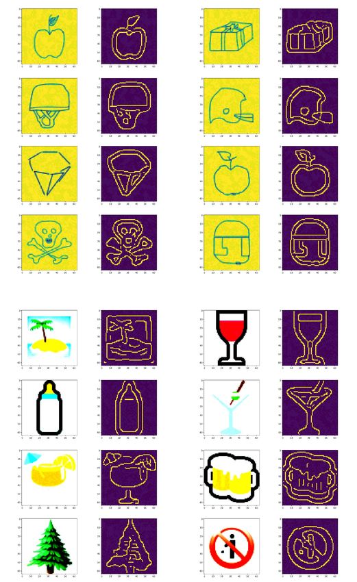
Under review as a conference paper at ICLR 2021

                                            FGSM                                                                     PGD-40
               adv. img - img    edge map      edge map adv.   diff. edge map                adv. img - img    edge map    edge map adv.   diff. edge map

e = 16

                                                                                e = 32
                           x20         DeepFool                                                          x20              CW

                                                                                steps=1000
steps=10

 Figure 1: Adversarial attacks against ResNet152 over the giant panda image using FGSM (Goodfellow
 et al., 2015), PGD-40 (Madry et al., 2017) (α=8/255), DeepFool (Moosavi-Dezfooli et al., 2016) and Carlini-
 Wagner (Carlini & Wagner, 2017) attacks. The second columns in panels show the difference (L2 ) between the
 original image (not shown) and the adversarial one (values shifted by 128 and clamped). The edge map (using
 Canny edge detector) remains almost intact at small perturbations. Notice that edges are better preserved for
 the PGD-40. See Appx. A for a more detailed version of this figure, and also the same using the Sobel method.
 There is no need for adversarial training (and hence less computation) in this method. Further, and
 perhaps less surprising, we find that incorporating edges also makes CNNs more robust to natural
 images corruptions and backdoor attacks. The versatility and effectiveness of these approaches,
 without significant parameter tuning, is very promising. Ultimately, our study shows that shape is the
 key to build robust models and opens a new direction for future research in adversarial robustness.

 2         R ELATED WORK
 Here, we provide a brief overview of the closely related research with an emphasis on adversarial
 defenses. For detailed comments on this topic, please refer to Akhtar & Mian (2018).
 Adversarial attacks. The goal of the adversary is to craft an adversarial input x̃ ∈ Rd by adding
 an imperceptible perturbation  to the (legitimate) input x ∈ Rd (here in the range [0,1]), i.e., x̃ =
 x + . Here, we consider two attacks based on the `∞ -norm of , the Fast Gradient Sign Method
 (FGSM) (Goodfellow et al., 2015), as well as the Projected Gradient Descent (PGD) method (Madry
 et al., 2017). Both white-box and black-box attacks in the untargeted condition are considered. Deep
 models are also susceptible to image transformations other than adversarial attacks (e.g., noise, blur),
 as is shown in Hendrycks & Dietterich (2019) and Azulay & Weiss (2018).
 Adversarial defenses. Recently, there has been a surge of methods to mitigate the threat from adver-
 sarial attacks either by making models robust to perturbations or by detecting and rejecting malicious
 inputs. A popular defense is adversarial training in which a network is trained on adversarial ex-
 amples (Szegedy et al., 2014; Goodfellow et al., 2015). In particular, adversarial training with a PGD
 adversary remains empirically robust to this day (Athalye et al., 2018). Drawbacks of adversarial
 training include impacting clean performance, being computationally expensive, and overfitting to
 the attacks it is trained on. Some defenses, such as Feature Squeezing (Xu et al., 2017), Feature
 Denoising (Xie et al., 2019), PixelDefend (Song et al., 2017), JPEG Compression (Dziugaite et al.,
 2016) and Input Transformation (Guo et al., 2017), attempt to purify the maliciously perturbed
 images by transforming them back towards the distribution seen during training. MagNet (Meng &
 Chen, 2017) trains a reformer network (one or multiple auto-encoders) to move the adversarial im-
 age closer to the manifold of legitimate images. Likewise, Defense-GAN (Samangouei et al., 2018)
 uses GANs (Goodfellow et al., 2014) to project samples onto the manifold of the generator before
 classifying them. A similar approach based on Variational AutoEncoders (VAE) is proposed in Li
 & Ji (2019). Unlike these works which are based on texture (and hence are fragile (Athalye et al.,
 2018)), our GAN-based defense is built upon edge maps. Some defenses are inspired by biology
 (e.g., Dapello et al. (2020), Li et al. (2019), Strisciuglio et al. (2020), Reddy et al. (2020)).
 Shape vs. texture. Geirhos et al. (2018) discovered that CNNs routinely latch on to the object
 texture, whereas humans pay more attention to shape. When presented with stimuli with conflicting
 cues (e.g., a cat shape with elephant skin texture; Appx. A), human subjects correctly labeled
 them based on their shape. In sharp contrast, predictions made by CNNs were mostly based on the
 texture (See also Hermann & Kornblith (2019)). Similar results are also reported by Baker et al.
 (2018). Hermann et al. (2020) studied the factors that produce texture bias in CNNs and learned
 that data augmentation plays a significant role to mitigate texture bias. Xiao et al. (2019), in parallel
 to our work, have also proposed methods to utilize shape for adversarial defense. They perform
 classification on the edge map rather than the image itself. This is a baseline method against which
 we compare our algorithms. Similar to us, they also use GANs to purify the input image.

                                                                            2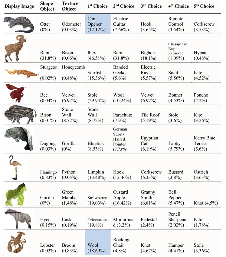
Under review as a conference paper at ICLR 2021

Algorithm 1 Edge-guided adversarial training (EAT) for T epochs, perturbation budget , and loss bal-
ance ratio α, over a dataset of size M for a network fθ (performed in minibatches in practice). β ∈
{edge, img, imgedge} indicates network type and redetect train means edge redetection during training.
    for t = 1 . . . T do
      for i = 1 . . . M do
         // launch adversarial attack (here FGSM and PGD attacks)
         x̃i = clip(xi +  sign(∇x `(fθ (xi ), yi )))
         if β == imgedge & redetect train then
             x̃i = detect edge(x̃i ) // recompute and replace the edge map
         end if
         ` = α `(fθ (xi ), yi ) + (1 − α) `(fθ (x̃i ), yi ) // here α = 0.5
         θ = θ − ∇θ ` // update model weights with some optimizer, e.g., Adam
      end for
    end for

Algorithm 2 GAN-based shape defense (GSD)
    // Training
        1. Create a dataset of images X = {xi , yi }i=1···N including clean and/or perturbed images
        2. Extract edge maps (ei ) for all images in the dataset
        3. Train a conditional GAN pg (x|e) to map edge image e to clean image x // here pix2pix
        4. Train a classifier pc (y|x) to map generated image x to class label y
    // Inference
        1. For input image x, clean or perturbed, first compute the edge image e
        2. Then, compute pc (y|x0 ) where x0 is the generated image corresponding to e

3       P ROPOSED METHODS
Edge-guided Adversarial Training (EAT). The intuition here is that the edge map retains the
structure in the image and helps disambiguate the classification (See Fig. 1). In its simplest form
(Fig. 7(A) in Appx. A; Alg. 1), adversarial training is performed over the 2D (Gray+Edge) or 4D
(RGB+Edge) input (i.e., number of channels; denoted as Img+Edge). In a slightly more complicated
form (Fig. 7(B)), first, for each input (clean or adversarial), the old edge map is replaced with the
newly extracted one. The edge map can be computed from the average of only image channels or all
available channels (i.e., image plus edge). The latter can sometimes improve the results, since the old
edge map (although perturbed; Fig. 10 and Appx. B) still contains unaltered shape structures. Then,
adversarial training is performed over the new input. The reason behind adversarial training with
redetected edges is to expose the network to possible image structure damage. The loss for training
is a weighted combination of loss over clean images and loss over adversarial images. At inference
time, first, the edge map is computed and then classification is done over the edge-augmented input.
As a baseline model, we also consider first detecting the input’s edge map and then feeding it to the
model trained on the edges for classification. We refer to this model as Img2Edge.
GAN-based Shape Defense (GSD). Here, first, a conditional GAN is trained to map the edge
image, from clean or adversarial images, to its corresponding clean image (Alg. 2). Any image
translation method (here pix2pix by Isola et al. (2017) using this code1 ) can be employed for this
purpose. Next, a CNN is trained over the generated images. At inference time, first, the edge map is
computed and then classification is done over the generated image for this edge image. The intuition
is that the edge map remains nearly the same over small perturbation budgets (See Appx. A). Notice
that conditional GAN can also be trained on perturbed images (similar to Samangouei et al. (2018)
and Li & Ji (2019) or edge-augmented perturbed images (similar to above).

4       E XPERIMENTS AND RESULTS
4.1       DATASETS AND M ODELS
Experiments are spread across 10 datasets covering a variety of stimulus types. Sample images from
datasets are given in Fig. 2. Models are trained with cross-entropy loss and Adam optimizer (Kingma
    1
        https://github.com/mrzhu-cool/pix2pix-pytorch

                                                        3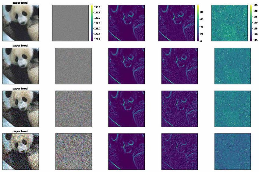
Under review as a conference paper at ICLR 2021

& Ba, 2014) with a batch size of 100, for 20 epochs over MNIST and FashionMNIST, 30 over
DogVsCat, and 10 over the remaining. Canny method (Canny, 1986) is used for edge detection over
all datasets, except DogBreeds for which Sobel is used. Edge detection parameters are separately
adjusted for each dataset. We did not carry out an exhaustive hyperparameter search, since we are
interested in additional benefits edges may bring rather than training the best possible models.
The first two datasets include MNIST (LeCun et al., 1998) and FashionMNIST (Xiao et al., 2017).
A CNN with 2 convolution, 2 pooling, and 2 fc layers is trained. Each of these datasets contains
60K training images (resolution 28×28) and 6K test images over 10 classes. The third dataset,
DogVsCat2 contains 18,085 training and 8,204 test images. Images in this dataset are of varying
dimensions. They are resized here to 150×150 pixels to save computation. A CNN with 4 convolu-
tion, 4 pooling, and 2 fc layers is trained from scratch.
                                    (10)   Fashion        (10)       Dog (16)     (2)       (43)    (50)      (250)    (10)    Tiny (200)
Over      the     remaining        MNIST   MNIST (10)   CIFAR10      Breeds     DogVsCat   GTSRB   Icons50   Sketch Imagenette ImageNet
datasets, we finetune a
pre-trained ResNet18 (He
et al., 2016), trained over
ImageNet (Deng et al.,
2009), and normalize im-
ages using ImageNet mean
and standard deviation.
The fourth dataset, CIFAR- Figure 2: Sample images from the datasets. Numbers in parentheses
10 (Krizhevsky, 2009), con- denote the number of classes.
tains 50K training and 10K test images with a resolution of 32×32 which are resized here to 64×64
for better edge detection. The fifth dataset is DogBreeds (see footnote). It contains 1,421 training
and 356 test images at resolution 224×224 over 16 classes. The sixth dataset is GTSRB (Stallkamp
et al., 2012) and includes 39,209 and 1,2631 training and test images, respectively, over 43 classes
(resolution 64×64 pixels). The seventh dataset, Icons-50, includes 6,975 training and 3,025 test
images over 50 classes (Hendrycks & Dietterich, 2019). The original image size is 120×120 which
is resized to 64×64. The eighth dataset, Sketch, contains 14K training and 6K test images over 250
classes. Images have size 1111×1111 and are resized to 64×64 in experiments (Eitz et al., 2012).
The ninth and tenth datasets are derived from ImageNet3 . The Imagenette2-160 dataset has 3,925
training and 9,469 test images (resolution 160×160) over 10 classes (tench, English springer, cas-
sette player, chain saw, church, French horn, garbage truck, gas pump, golf ball, and parachute).
The Tiny Imagenet dataset has 100K training images (resolution 64 × 64) and 10K validation images
(used here as the test set) over 200 classes.
For attacks, we use https://github.com/Harry24k/adversarial-attacks-pytorch, ex-
cept Boundary attack for which we use https://github.com/bethgelab/foolbox.

4.2      R ESULTS
4.2.1 E DGE - GUIDED A DVERSARIAL T RAINING
Results over MNIST and CIFAR-10 are shown in Tables 1 and 2, respectively. In these experi-
ments, edge maps are computed only from the gray-level image (in turn computed from the image
channels). Please refer to Appx. B for results over the remaining datasets.
Over MNIST and FashionMNIST, robust models trained using edges outperform models trained on
gray-level images (the last column). The naturally trained models, however, perform better using
gray-level images than edge maps (Orig. model column). Adversarial training with augmented
inputs improves the robustness significantly over both datasets, except the FGSM attack on Fashion-
MNIST. Over CIFAR-10, incorporating the edges improves the robustness by a large margin against
the PGD-40 attack. At  = 32/255, the performance of the robust model over clean and perturbed
images is raised from (0.316, 0.056) to (0.776, 0.392). On average, the robust model shows 64%
improvement over the RGB model (last column in Table 2). Results when using the Sobel edge
detector instead of the Canny does not show a significant difference (Table 7 in Appx. B). Over the
TinyImageNet dataset, as in CIFAR-10, classification using edge maps is poor perhaps due to the
background clutter. Nevertheless, incorporating edges improves the results. We expect even better
   2
       www.kaggle.com/c/dogs-vs-cats-redux-kernels-edition & www.kaggle.com/c/dog-breed-identification
   3
       https://github.com/fastai/imagenette & https://tiny-imagenet.herokuapp.com

                                                                 4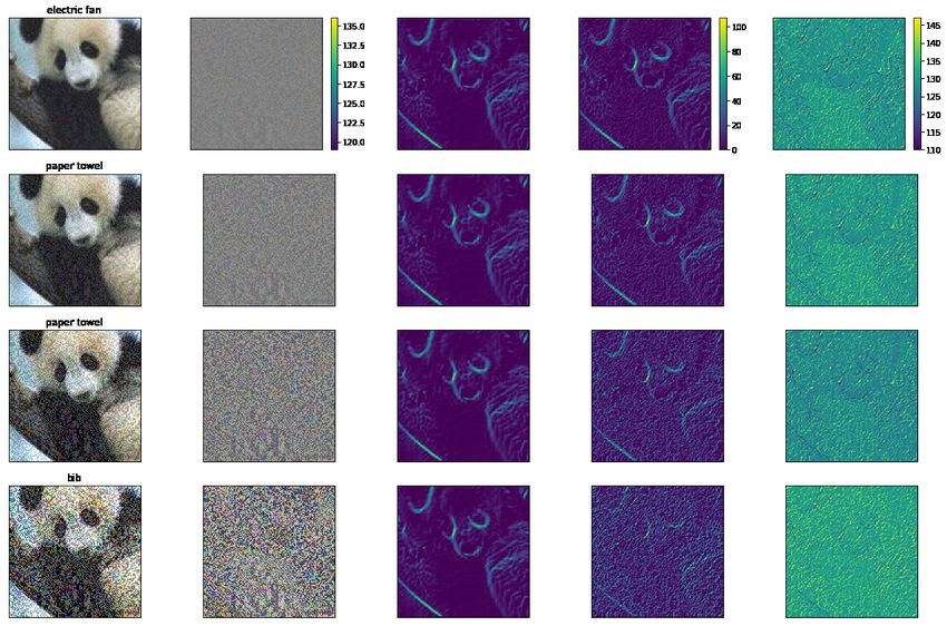
Under review as a conference paper at ICLR 2021

Table 1: Results (Top-1 acc) over MNIST. The best accuracy in each column is highlighted in bold. In italics
are the results of the substitute attack. Epsilon values are over 255. We used the `∞ variants of FGSM and
PGD. Img2Edge means applying the Edge model (first row) to the edge map of the image.
                                   Orig. model               Rob. model (8)          Rob. model (32)         Rob. model (64)       Average
                        0/clean     8     32      64     0/clean 8               0/clean 32              0/clean 64              Rob. models
          Edge         0.964 0.925 0.586          0.059   0.973   0.954           0.970   0.892           0.964   0.776                0.921
          Img2Edge       ,,   0.960 0.951         0.918   ,,      0.971           ,,      0.957           ,,      0.910                0.957
 FGSM

          Img          0.973 0.947 0.717          0.162   0.976   0.955           0.977   0.892           0.970   0.745                0.919
          Img+Edge 0.972 0.941 0.664              0.089   0.976   0.958           0.977   0.902           0.972   0.782                0.928
          Redetect       ”    0.950 0.803         0.356   ”       0.962 (0.968)   ”       0.919 (0.947)   ”       0.843 (0.881)        0.941
                   Img + Redetected Edge                  0.974   0.950           0.970   0.771           0.968   0.228                0.810
                          Redetect                        ”       0.958 (0.966)   ”       0.929 (0.947)   ”       0.922 (0.925)        0.953
          Edge         0.964 0.923 0.345          0.000   0.971   0.949           0.973   0.887           0.955   0.739                0.912
          Img2Edge       ,,   0.961 0.955         0.934   ,,      0.970           ,,      0.958           ,,      0.927                0.960
 PGD-40

          Img          0.973 0.944 0.537          0.008   0.977   0.957           0.978   0.873           0.963   0.658                0.901
          Img+Edge 0.972 0.938 0.446              0.001   0.978   0.953           0.975   0.879           0.965   0.743                0.915
          Redetect       ”    0.950 0.741         0.116   ”       0.960 (0.967)   ”       0.913 (0.948)   ”       0.804 (0.908)        0.932
                   Img + Redetected Edge                  0.975   0.949           0.973   0.649           0.968   0.000                0.752
                          Redetect                        ”       0.958 (0.967)   ”       0.945 (0.958)   ”       0.939 (0.942)        0.960

                                                 Table 2: Results over the CIFAR-10 dataset.
                                           Orig. model                  Rob. model (8)             Rob. model (32)         Average
                                    0/clean     8     32          0/clean 8                   0/clean 32                 Rob. models
                     Edge           0.490    0.060        0.015    0.535       0.323           0.382      0.199                0.360
                     Img2Edge         ,,     0.258        0.258    ,,          0.270           ,,         0.217                0.351
            FGSM

                     Img            0.887    0.359        0.246    0.869       0.668           0.855      0.553                0.736
                     Img + Edge     0.860    0.366        0.169    0.846       0.611           0.815      0.442                0.679
                     Redetect         ,,     0.399        0.281    ,,          0.569 (0.631)   ,,         0.417 (0.546)        0.662
                             Img + Redetected Edge                 0.846       0.530           0.832      0.337                0.636
                                    Redetect                       ,,          0.702 (0.753)   ,,         0.569 (0.678)        0.737
                     Edge           0.490    0.071        0.000    0.537       0.315           0.142      0.119                0.278
                     Img2Edge         ,,     0.259        0.253    ,,          0.274           ,,         0.253                0.301
            PGD-40

                     Img            0.887    0.018        0.000    0.807       0.450           0.316      0.056                0.407
                     Img + Edge     0.860    0.019        0.000    0.788       0.429           0.176      0.119                0.378
                     Redetect         ,,     0.306        0.093    ,,          0.504 (0.646)   ,,         0.150 (0.170)        0.404
                             Img + Redetected Edge                 0.834       0.155           0.776      0.006                0.443
                                    Redetect                       ,,          0.661 (0.767)   ,,         0.392 (0.700)        0.666

results with more accurate edge detection algorithms (e.g., supervised deep edge detectors). Over
these 4 datasets, the final model (i.e., adversarial training using image + redetected edge, and edge
redetection at inference time) leads to the best accuracy. The improvement over the image is more
pronounced at larger perturbations, in particular against the PGD-40 attack (as expected; Fig. 1).
Over the DogVsCat dataset, as in FashionMNIST, the model trained on the edge map is much more
robust than the image-only model (Table 8 in Appx. B). Over the DogBreeds dataset, utilizing edges
does not improve the results significantly (compared to the image model). The reason could be
that texture is more important than shape in this fine-grained recognition task (Table 9 Appx. B).
Over GTSRB, Icons-50, and Sketch datasets, image+edge model results in higher robustness than
the image-only model, but leads to relatively less improvement compared to the edge-only model.
Please see Tables 11, 13, and 15. Over the Imagenette2-160 dataset (Table 17), classification using
images does better than edges since the texture is very important on this dataset.
Average results over 10 datasets is presented in Fig. 3 (left panel). Combining shape and texture
(full model) leads to a substantial improvement in robustness over the texture alone (5.24% imp.
against FGSM and 28.76% imp. against PGD-40). Also, image+edge model is slightly more robust
than the image-only model. Computing the edge map from all image channels improves the results
on some datasets (e.g., GTSRB and Sketch) but hurts on some others (e.g., CIFAR-10) as shown
in Appx. B. The right two panels in Fig. 3 show a comparison of natural (Orig. model column in
tables; solid lines) vs. adversarial training. Natural training with image+edge and redetection at
inference time leads to enhanced robustness with little to no harm to standard accuracy. Despite the
Edge model only being trained on edges from clean images, the Img2Edge model does better than
other naturally-trained models against attacks. The best performance, however, belongs to models
trained adversarially. Notice that our results set a new record on adversarial robustness on some of
these datasets even without exhaustive parameter search4 .
Robustness against Carlini-Wagner (CW) and Boundary attacks. Performance of our method
against l2 CW attack on MNIST dataset is shown in Appx. J. To make experiments tractable, we
set the number of attack iterations to 10. With even 10 iterations, the original Edge and Img mod-

      4
          cf. Zhang et al. (2019); the best robust accuracy on CIFAR-10 against PGD attacks is under 60%.

                                                                           5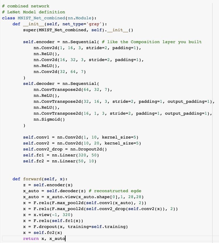
Under review as a conference paper at ICLR 2021

                                                                   FGSM                              PGD-40

Figure 3: Left) Average results of the EAT defense on all datasets (last cols. in tables). Middle and Right)
Comparison of natural (Orig. model column; solid lines) vs. adversarial training averaged over all datasets.
els are severely degraded. Img2Edge and Img+(Edge Redetect) models, however, remain robust.
Adversarial training with CW attack results in robust models in all cases.
Results against the decision-based Boundary attack (Brendel et al., 2017) are shown in Appx. K over
MNIST and Fashion MNIST datasets. Edge, Img, and Img+Edge models perform close to zero over
adversarial images. Img+(Edge Redetect) model remains robust since the Canny edge map does not
change much after the attack, as is illustrated in Fig. 29.
Robustness against substitute model attacks. Following Papernot et al. (2016), we trained substi-
tute models to mimic the robust models (with the same architecture but with RGB channels) using
the cross-entropy loss over the logits of the two networks, for 5 epochs. The adversarial examples
crafted for the substitute networks were then fed to the robust networks. Results are shown in italics
in Tables 1, 2, 4 and 5 (performed only against the edge-redetect models). We find that this attack is
not able to knock off the robust models. Surprisingly, it even improves the accuracy in some cases.
Please refer to Appx. E for more details.
Robustness against adaptive attacks. So far we have been using the Canny edge detector which
is non-differentiable. What if the adversary builds a differentiable edge detector to approximate the
Canny edge detector and then utilizes it to craft adversarial examples? To study this, we run two
experiments. In the first one, we build the following pipeline using the HED deep edge detector (Xie
& Tu, 2015): Img −→ HED −→ ClassifierHED . A CNN classifier (as above) is trained over the
HED edges on the Imagenette2-160 dataset (See Appx. L). Attacking this classifier with FGSM and
PGD-5 ( = 8/255) completely fools the network. The original classifier (Img2Edge here) trained
on Canny edges, however, is still largely robust to the attacks (i.e., Imgadv−HED −→ Canny −→
ClassifierCanny ) as shown in Table 29. Notice that the HED edge maps are continuous in the range
[0,1], whereas Canny edge maps are binary, which may explain why it is easy to fool the HED
classifier (See Fig. 30).
Above, we used an off the shelf deep edge detector trained on natural scenes. As can be seen in
Appx. L, its generated edge maps differ significantly from Canny edges. What if the adversary
trains a model with the (input, output) pair as (input image, Canny edge map) to better approximate
the Canny edge detector? In experiment two, we investigate this possibility. We build a pipeline con-
sisting of a convolutional autoencoder followed by a CNN on MNIST. Details regarding architecture
and training procedure are given in Appx. M. As results in Fig. 33 reveal, FGSM and PGD-40 at-
tacks against the pipeline are very effective. Passing the adversarial images through Canny and then
a trained (naturally or adversarially) classifier on Canny edges (i.e., Img2Edge), still leads to high
accuracy, which means that transfer was not successful. We attribute this feat to the binary output of
Canny. Two important point deserve attention. First, here we used the Img2Edge model, which as
shown above, is less robust compared to the full model (i.e., img+edge and redetection). Thus, adap-
tive attacks may be even less effective against the full model. Second, proposed methods perform
better when edge map is less disturbed. For example, as shown in Fig. 33 (bottom), the adaptive
attack is less effective against the PGD attack since edges are preserved better.
Analysis of parameter α. By setting α = 0, the network will be exposed only to adversarial
examples (Alg. 1), which is computationally more efficient. However, it results in lower accuracy
and robustness compared to when α = 0.5, which means exposing the network to both clean and
adversarial images is important (See Table 19; Appx. D). Nevertheless, here again incorporating
edges improves the robustness significantly compared to the image-only case.
Why is this method working? The main reason is that the edge map acts as a checksum, and
the network learns (through adversarial training) to rely more on the redetected edges when other

                                                       6
Under review as a conference paper at ICLR 2021

channels are misleading (See Table 23). This aligns with prior observations such as shortcut learning
in CNNs (Geirhos et al., 2020). Also, our approach resembles adversarial patch or backdoor/trojan
attacks where the goal is to fool a classifier by forcing it to rely on irrelevant cues. Conversely, here
we use this trick to make a model more robust. Also, the Img2Edge model can purify the input
before classifying it. Any adaptive attack against the EAT defense has to alter the edges which most
likely will result in perceptible structural damages. See also Figs. 10 & 14 in Appx. A.
4.2.2   GAN- BASED S HAPE DEFENSE
We trained the pix2pix model for 10 epochs over MNIST and FashionMNIST, and for 100 epochs
over CIFAR-10 and Icons-50 datasets. Sample generated images are shown in Fig. 18 (Appx. F).
A CNN (same architecture as before) was trained for 10 epochs to classify the generated images.
Results are shown in Fig. 4. The model trained over the images generated by pix2pix (solid lines
in the figure) is compared to the model trained over the original clean training set (denoted by the
dashed lines). Both models are tested over the clean and perturbed versions of the original test sets of
the four datasets. Over MNIST and FashionMNIST datasets, GSD performs on par with the original
model on clean test images. It is, however, much more robust than the original model against the
attacks. When we trained the pix2pix over the edge maps from the perturbed images, the new CNN
models became even more robust (stars in Fig. 4; top panels). We expect even better results with
training over edge maps from both intact and perturbed images5 .
Over CIFAR-10 and Icons-50 datasets, generated im-
ages are poor. Consequently, GSD underperforms the
original model over the original clean images. Over
the adversarial inputs, however, GSD wins, especially
at high perturbation budgets and against the PGD-40 at-
tack. With better edge detection and image generation
methods (e.g., using perceptual loss), even better results
are expected.
Why is this method working? The main reason is that
cGAN learns a function f that is invariant to adversar-
ial perturbations. Since the edge map is not completely
invariant to (especially large) perturbations, one has to
train the cGAN on the augmented dataset composed of
clean and perturbed images. One advantage of this ap-
proach is it computational efficiency since there is no
need for adversarial training. Any adaptive attack against
this defense has to fool the cGAN which is perhaps not
feasible since it will be noticed from the generated im-
ages (i.e., cGAN will fail to generate decent images).             Figure 4: Results of GSD method.
Compared to other adversarial defenses that utilize GANs (e.g., Samangouei et al. (2018); Li &
Ji (2019)), our approach relies less on texture. It can be integrated with these defenses.

5 FAST & FREE ADVERSARIAL TRAINING WITH SHAPE DEFENSE
Here, we examine whether incorporating shape bias can empower other defenses, in particular,
a) fast adversarial training by Wong et al. (2020), dubbed FastAT, and free adversarial training
by Shafahi et al. (2019), dubbed FreeAT. Wong et al. trained robust models using a much weaker
and cheaper adversary to lower the cost of adversarial training. They showed that adversarial training
with the FGSM adversary is as effective as PGD-based training. The key idea in Shafahi et al. ’s work
is to simultaneously update both the model parameters and image perturbations in one backward
pass, rather than using separate gradient computations at each update step. Please see also Appx. G.
The same CNN architectures as in Wong et al. are employed here. For FastAT, we trained three
models over MNIST (for 10 epochs), FashionMNIST (for 3 epochs), and CIFAR-10 (for 10 epochs
& early-stopping) datasets. For FreeAT, we trained models only over CIFAR-10 for 10 epochs.
Results are shown in Table 3. Using shape-based FastAT and over MNIST, robust accuracy against
PGD-50 grows from 95.5% (image-only model) to 98.4% (our full model) at  = 0.1 and from
    5
      Similarly, the edge map classifier used in the Img2Edge model in the previous section (EAT defense) can
be trained on edge maps from both clean and adversarial examples to improve performance.

                                                     7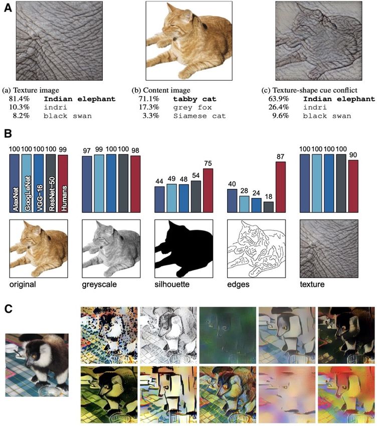
Under review as a conference paper at ICLR 2021
Table 3: Performance of edge-augmented FastAT and FreeAT adversarial defenses over clean and perturbed
images (See Appx. G for extended algorithms). FastAT is trained with the FGSM adversary ( = 0.1 or
= 0.3) over MNIST and FashionMNIST datasets, and = 8/255 over CIFAR-10). FreeAT is trained over
CIFAR-10 with = 8/255 and 8 minibatch replays. CIFAR-10 results are averaged over 3 runs (Appx. G).
PGD attacks use 10 random restarts. The remaining settings and parameters are as in Wong et al. (2020).
MNIST (FastAT) Fashion MNIST (FastAT) CIFAR-10 (FastAT) CIFAR-10 (FreeAT)
0.1 0.3 Avg. 0.1 0.3 Avg. 8/255 Avg. 8/255 Avg.
0 PGD-50 0 PGD-50 Acc. 0 PGD-50 0 PGD-50 Acc. 0 PGD-10 Acc. 0 PGD-10 Acc.
Edge 0.986 0.940 0.113 0.113 0.538 0.844 0.753 0.786 0.110 0.623 0.582 0.386 0.484 0.679 0.678 0.678
Img 0.991 0.955 0.985 0.877 0.952 0.835 0.696 0.641 0.000 0.543 0.767 0.381 0.574 0.774 0.449 0.612
Img + Edge 0.988 0.968 0.980 0.922 0.965 0.851 0.780 0.834 0.769 0.809 0.874 0.386 0.630 0.782 0.442 0.612
Redetect ,, 0.977 ,, 0.966 0.978 ,, 0.823 ,, 0.778 0.822 ,, 0.393 0.634 ,, 0.448 0.615
Img + Red. Edge 0.986 0.087 0.986 0.000 0.515 0.857 0.262 0.817 0.000 0.484 0.866 0.074 0.470 0.777 0.451 0.614
Redetect ,, 0.984 ,, 0.986 0.986 ,, 0.855 ,, 0.823 0.838 ,, 0.416 0.641 ,, 0.452 0.615
87.7% to 98.6% at = 0.3, which are even higher than what is reported by Wong et al. (97.5% at
= 0.1 and 88.8% at = 0.3). Over FashionMNIST, the improvement is even more pronounced
(from 69.6% to 85.5% at = 0.1 and from 0% to 82.3% at = 0.3 ). Over clean images, our full
model outperforms other models in most of the cases. Over the CIFAR-10 dataset, the shape-based
extension of the defenses results in high accuracy over both clean and perturbed images (using PGD-
10 attack), compared to the image-only model. We expect similar improvements with the classic
PGD adversarial training. Overall, our analyses in this section suggest that exploiting edges is not
specific to the particular way we perform adversarial training (Algorithms 1&2), and be extended to
other defense methods (e.g., TRADES algorithm by Zhang et al. (2019)).
6 BACKGROUND SUBTRACTION
Background subtraction (a.k.a foreground detection) is an important mechanism by which humans
process scenes and recognize objects. It interacts with other mechanisms such as edge and boundary
detection. How useful is it for adversarial robustness? In other words, how robust the model will
be assuming that the attacker has only access to the foreground object? To find out, we perform an
experiment over MNIST and FashionMNIST, for which it is easy to derive the foreground masks. We
compare the Img and Edge models (from Section 4.2.1) over the original and noisy (digits placed
on white noise background) data, with and without background subtraction and edge detection,
against the FGSM attack. Results are shown in Fig. 5(A). First, both models perform poorly over
noisy images with the Edge model doing better. Second, post background subtraction, models are
much more robust. Third, applying the Edge model to the foreground region leads to almost perfect
robustness over MNIST. Even without perfect edge detection, the Edge model does very well over
FashionMNIST. This analysis provides an upper bound on the potential benefit from background
subtraction on model robustness, assuming that foreground objects can be reliably detected.
7 H ARNESSING BACKDOOR ATTACKS
Proposed mechanisms can also withstand invisible and visible backdoor attacks (Brown et al., 2017;
Liu et al., 2017). Over MNIST, we planted an invisible C-like patch in half of the 8s and relabeled
them as 9. We then trained the Img model on this new dataset. The Img model on a test set where all
8s are contaminated (with the patch), classifies almost all of them as 9 (top-left panel in Fig. 5.B).
The Edge model, however, correctly classifies them as 8 since edge detection removes the pattern
(top-right panel). Thanks to the edge detection, it is also not possible to train the Edge model on the
poisoned dataset. A similar experiment on FashionMNIST, using a different patch, shows similar
results (bottom panels in Fig. 5.B). In presence of visible patches, the model would not be affected
if the correct region is identified (via background subtraction) during training or testing (Appx. I).
8 ROBUSTNESS AGAINST NATURAL IMAGE DISTORTIONS
Previous work has shown that ImageNet-trained CNNs generalize poorly over a wide range of image
distortions (e.g., Azulay & Weiss (2018); Dodge & Karam (2017)). Our objective in this section is to
study whether increasing shape bias improves robustness against common image distortions just as
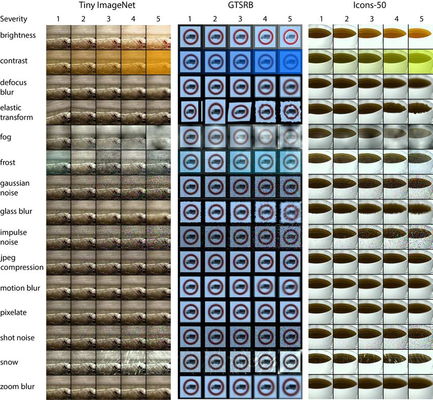
it did over adversarial examples. Following Hendrycks & Dietterich (2019), we systematically test
how model accuracies degrade if images are corrupted by 15 different types of distortions including
brightness, contrast, defocus blur, elastic transform, fog, frost, Gaussian noise, glass blur, impulse
noise, JPEG compression, motion blur, pixelatation, shot noise, snow, and zoom blur, at 5 levels of
severity. Fig. 19 (Appx. H) shows sample images along with their distortions.
We test the original models (trained naturally on clean training images) as well as the robust
models (trained adversarially using Algorithm 1) over the corrupted versions of test sets on three
8
Under review as a conference paper at ICLR 2021

A                                                                      e = 0.2
                                                                                   B      acc=90.33
                                                                                          (test - Img)
                                                                                                              acc=95.97
                                                                                                              (test- Edge)

                                                     image

                                                                                 8 -> 9
             RED = Img model

                                                                                  Pred
             BLUE = Edge model

                                                     + noise
                                                     + perturbed
                                                                                          acc=80.04           acc=74.08
                                                                                          (test - Img)        (test- Edge)

                                                  perturbed
                                                     (fg)

                                                                                 2 -> 5
                                                                                  Pred
                                                  (fg & edge)
                                                  perturbed
                                                                                                         gt                  gt
Figure 5: A) Background subtraction together with edge detection improves robustness (here against the
FGSM attack). Noisy data is created by overlaying a digit over white noise (noise×(1-mask)+digit). B) De-
fending backdoor attacks. An almost invisible pattern (with intensity 10/255 of the digit intensity) is added to
half of the samples from one class, which are then relabeled as another class. Notice that the Edge model is
not confused over the edge maps (right panels) since edge detection removes the pattern. In case of a visible
backdoor attack, background subtraction can help discard the irrelevant region. See Appx. I for more details.

datasets. Results are visualized in Fig. 6. See Appx. H for breakdown results on each dataset
and distortion. Two conclusions are drawn. First, incorporating edge information in origi-
nal models (and hence increasing shape bias) improves robustness against common image dis-
tortions (solid curves in Fig. 6; RGB+Egde > RGB or Edge). Improvement is more notice-
able at larger distortions and over datasets with less background clutter (e.g., Icons-50). This is
in alignment with Geirhos et al. (2018) where they showed ResNet-50 trained on the Stylized-
ImageNet dataset performs better than the vanilla ResNet-50 on both clean and distorted images.
Second, adversarially-trained mod-
els (in particular those trained on
Img + Edge) are more robust to im-
age distortions compared to orig-
inal models. In summary, incor-
porating edges and adversarial im-
ages leads to improved robustness
against natural image distortions,
despite models not being trained on
any of the distortions during train-
ing. This in turn suggests that the
proposed algorithms indeed rely
more on shape than texture.            Figure 6: Classification accuracy over naturally distorted images.

9    D ISCUSSION AND OUTLOOK
Two algorithms are proposed to use shape bias and background subtraction to strengthen CNNs and
defend against adversarial attacks and backdoor attacks. To fool these defenses one has to perturb the
image such that the new edge map is significantly different from the old one while preserving image
shape and geometry, which does not seem to be trivial at low perturbation budgets. Even though
we did not perform an exhaustive parameter search (model architecture, epochs, edge detection,
cGAN training, etc.), our results are better than or on par with the state of the art in some cases
(e.g., over MNIST and CIFAR datasets). The proposed mechanisms are computationally efficient
and excel with higher resolution images and low background clutter. They are also more effective
against stronger attacks than weaker ones since strong attacks perturb the image less while being
more destructive (e.g., PGD vs. FGSM; Fig. 1). Shape defense can also be combined with other
defenses to produce robust models without a significant slowdown.
Future work should assess shape defense against adversarial attacks such as e.g., gradient-free at-
tacks, decision-based attacks, sparse attacks (e.g., the one pixel attack (Su et al., 2019)), attacks
that perturb only the edge pixels, attacks that manipulate the image structure (Xiao et al., 2018),
ad-hoc adaptive attacks, , and backdoor (Chen et al., 2017)), as well as other `p norms, and datasets.
There might be also other ways to incorporate shape-bias in CNNs, such as 1) augmenting a dataset
with edge maps or negative images, 2) overlaying texture from some objects onto some others as
in Geirhos et al. (2018), and 3) designing normalization layers (Carandini & Heeger, 2012). Lastly,
the interpretation of the shape defense, as in Zhang & Zhu (2019), is another research direction.

                                                                   9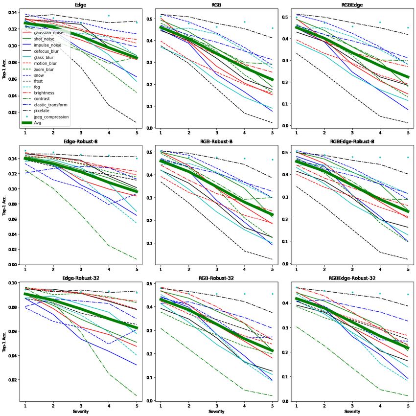
Under review as a conference paper at ICLR 2021

R EFERENCES
Naveed Akhtar and Ajmal Mian. Threat of adversarial attacks on deep learning in computer vision:
  A survey. IEEE Access, 6:14410–14430, 2018.
Anish Athalye, Nicholas Carlini, and David A. Wagner. Obfuscated gradients give a false sense of
  security: Circumventing defenses to adversarial examples. CoRR, abs/1802.00420, 2018.
Aharon Azulay and Yair Weiss. Why do deep convolutional networks generalize so poorly to small
  image transformations? arXiv preprint arXiv:1805.12177, 2018.
Nicholas Baker, Hongjing Lu, Gennady Erlikhman, and Philip J Kellman. Deep convolutional
  networks do not classify based on global object shape. PLoS computational biology, 14(12):
  e1006613, 2018.
Irving Biederman. Recognition-by-components: a theory of human image understanding. Psycho-
   logical review, 94(2):115, 1987.
Wieland Brendel, Jonas Rauber, and Matthias Bethge. Decision-based adversarial attacks: Reliable
 attacks against black-box machine learning models. arXiv preprint arXiv:1712.04248, 2017.
Tom B Brown, Dandelion Mané, Aurko Roy, Martı́n Abadi, and Justin Gilmer. Adversarial patch.
  arXiv preprint arXiv:1712.09665, 2017.
John Canny. A computational approach to edge detection. IEEE Transactions on pattern analysis
  and machine intelligence, (6):679–698, 1986.
Matteo Carandini and David J Heeger. Normalization as a canonical neural computation. Nature
 Reviews Neuroscience, 13(1):51–62, 2012.
Nicholas Carlini and David A. Wagner. Towards evaluating the robustness of neural networks. In
  IEEE Symposium on Security and Privacy, pp. 39–57, 2017.
Xinyun Chen, Chang Liu, Bo Li, Kimberly Lu, and Dawn Song. Targeted backdoor attacks on deep
  learning systems using data poisoning. arXiv preprint arXiv:1712.05526, 2017.
Joel Dapello, Tiago Marques, Martin Schrimpf, Franziska Geiger, David D Cox, and James J Di-
  Carlo. Simulating a primary visual cortex at the front of cnns improves robustness to image
  perturbations. BioRxiv, 2020.
Jia Deng, Wei Dong, Richard Socher, Li-Jia Li, Kai Li, and Li Fei-Fei. Imagenet: A large-scale hi-
   erarchical image database. In 2009 IEEE conference on computer vision and pattern recognition,
   pp. 248–255. Ieee, 2009.
Samuel Dodge and Lina Karam. A study and comparison of human and deep learning recogni-
  tion performance under visual distortions. In 2017 26th international conference on computer
  communication and networks (ICCCN), pp. 1–7. IEEE, 2017.
Gintare Karolina Dziugaite, Zoubin Ghahramani, and Daniel Roy. A study of the effect of JPG
  compression on adversarial images. CoRR, abs/1608.00853, 2016.
Mathias Eitz, James Hays, and Marc Alexa. How do humans sketch objects? ACM Trans. Graph.
 (Proc. SIGGRAPH), 31(4):44:1–44:10, 2012.
Robert Geirhos, Patricia Rubisch, Claudio Michaelis, Matthias Bethge, Felix A Wichmann, and
  Wieland Brendel. Imagenet-trained cnns are biased towards texture; increasing shape bias im-
  proves accuracy and robustness. arXiv preprint arXiv:1811.12231, 2018.
Robert Geirhos, Jörn-Henrik Jacobsen, Claudio Michaelis, Richard Zemel, Wieland Brendel,
  Matthias Bethge, and Felix A Wichmann. Shortcut learning in deep neural networks. arXiv
  preprint arXiv:2004.07780, 2020.
Ian Goodfellow, Jean Pouget-Abadie, Mehdi Mirza, Bing Xu, David Warde-Farley, Sherjil Ozair,
  Aaron Courville, and Yoshua Bengio. Generative adversarial nets. In Advances in neural infor-
  mation processing systems, pp. 2672–2680, 2014.

                                               10
Under review as a conference paper at ICLR 2021
Ian Goodfellow, Jonathon Shlens, and Christian Szegedy. Explaining and harnessing adversarial
examples. In Proc. ICLR, 2015.
Chuan Guo, Mayank Rana, Moustapha Cissé, and Laurens van der Maaten. Countering adversarial
images using input transformations. CoRR, abs/1711.00117, 2017.
Kaiming He, Xiangyu Zhang, Shaoqing Ren, and Jian Sun. Deep residual learning for image recog-
nition. In Proceedings of the IEEE conference on computer vision and pattern recognition, pp.
770–778, 2016.
Dan Hendrycks and Thomas Dietterich. Benchmarking neural network robustness to common cor-
ruptions and perturbations. arXiv preprint arXiv:1903.12261, 2019.
Katherine Hermann, Ting Chen, and Simon Kornblith. The origins and prevalence of texture bias in
convolutional neural networks. Advances in Neural Information Processing Systems, 33, 2020.
Katherine L Hermann and Simon Kornblith. Exploring the origins and prevalence of texture bias in
convolutional neural networks. arXiv preprint arXiv:1911.09071, 2019.
Phillip Isola, Jun-Yan Zhu, Tinghui Zhou, and Alexei A Efros. Image-to-image translation with
conditional adversarial networks. In Proceedings of the IEEE conference on computer vision and
pattern recognition, pp. 1125–1134, 2017.
Laurent Itti and Christof Koch. Computational modelling of visual attention. Nature reviews neuro-
science, 2(3):194–203, 2001.
Diederik Kingma and Jimmy Ba. Adam: A method for stochastic optimization. CoRR,
abs/1412.6980, 2014.
Nikolaus Kriegeskorte. Deep neural networks: a new framework for modeling biological vision and
brain information processing. Annual review of vision science, 1:417–446, 2015.
Alex Krizhevsky. Learning multiple layers of features from tiny images, 2009.
Alex Krizhevsky, Ilya Sutskever, and Geoffrey E Hinton. Imagenet classification with deep convo-
lutional neural networks. In Advances in neural information processing systems, pp. 1097–1105,
2012.
Yann LeCun, Léon Bottou, Yoshua Bengio, and Patrick Haffner. Gradient-based learning applied to
document recognition. Proc. IEEE, 1998.
Yann LeCun, Yoshua Bengio, and Geoffrey Hinton. Deep learning. Nature, 521(7553):436–444,
2015.
Xiang Li and Shihao Ji. Defense-vae: A fast and accurate defense against adversarial attacks. In
Joint European Conference on Machine Learning and Knowledge Discovery in Databases, pp.
191–207. Springer, 2019.
Zhe Li, Wieland Brendel, Edgar Walker, Erick Cobos, Taliah Muhammad, Jacob Reimer, Matthias
Bethge, Fabian Sinz, Zachary Pitkow, and Andreas Tolias. Learning from brains how to regularize
machines. In Advances in Neural Information Processing Systems, pp. 9529–9539, 2019.
Yingqi Liu, Shiqing Ma, Yousra Aafer, Wen-Chuan Lee, Juan Zhai, Weihang Wang, and Xiangyu
Zhang. Trojaning attack on neural networks. 2017.
Aleksander Madry, Aleksandar Makelov, Ludwig Schmidt, Dimitris Tsipras, and Adrian Vladu.
Towards deep learning models resistant to adversarial attacks. CoRR, abs/1706.06083, 2017.
Dongyu Meng and Hao Chen. Magnet: A two-pronged defense against adversarial examples. In
Proceedings of the 2017 ACM SIGSAC Conference on Computer and Communications Security,
CCS 2017, Dallas, TX, USA, October 30 - November 03, 2017, pp. 135–147, 2017. doi: 10.1145/
3133956.3134057.
Seyed-Mohsen Moosavi-Dezfooli, Alhussein Fawzi, and Pascal Frossard. Deepfool: A simple and
accurate method to fool deep neural networks. In Proc. CVPR, pp. 2574–2582, 2016.
11Under review as a conference paper at ICLR 2021
Nicolas Papernot, Patrick McDaniel, Ian Goodfellow, Somesh Jha, Z Berkay Celik, and Ananthram
Swami. Practical black-box attacks against deep learning systems using adversarial examples.
CoRR, abs/1602.02697, 2016.
Manish Vuyyuru Reddy, Andrzej Banburski, Nishka Pant, and Tomaso Poggio. Biologically inspired
mechanisms for adversarial robustness. Advances in Neural Information Processing Systems, 33,
2020.
Pouya Samangouei, Maya Kabkab, and Rama Chellappa. Defense-gan: Protecting classifiers against
adversarial attacks using generative models. arXiv preprint arXiv:1805.06605, 2018.
Ali Shafahi, Mahyar Najibi, Mohammad Amin Ghiasi, Zheng Xu, John Dickerson, Christoph
Studer, Larry S Davis, Gavin Taylor, and Tom Goldstein. Adversarial training for free! In
Advances in Neural Information Processing Systems, pp. 3358–3369, 2019.
Yang Song, Taesup Kim, Sebastian Nowozin, Stefano Ermon, and Nate Kushman. Pixeldefend:
Leveraging generative models to understand and defend against adversarial examples. arXiv
preprint arXiv:1710.10766, 2017.
Johannes Stallkamp, Marc Schlipsing, Jan Salmen, and Christian Igel. Man vs. computer: Bench-
marking machine learning algorithms for traffic sign recognition. Neural networks, 32:323–332,
2012.
Nicola Strisciuglio, Manuel Lopez-Antequera, and Nicolai Petkov. Enhanced robustness of con-
volutional networks with a push–pull inhibition layer. Neural Computing and Applications, pp.
1–15, 2020.
Jiawei Su, Danilo Vasconcellos Vargas, and Kouichi Sakurai. One pixel attack for fooling deep
neural networks. IEEE Transactions on Evolutionary Computation, 23(5):828–841, 2019.
Christian Szegedy, Wojciech Zaremba, Ilya Sutskever, Joan Bruna, Dumitru Erhan, Ian Goodfellow,
and Rob Fergus. Intriguing properties of neural networks. In In Proc. ICLR, 2014.
Eric Wong, Leslie Rice, and J Zico Kolter. Fast is better than free: Revisiting adversarial training.
arXiv preprint arXiv:2001.03994, 2020.
Chaowei Xiao, Jun-Yan Zhu, Bo Li, Warren He, Mingyan Liu, and Dawn Song. Spatially trans-
formed adversarial examples. arXiv preprint arXiv:1801.02612, 2018.
Chaowei Xiao, Mingjie Sun, Haonan Qiu, Han Liu, Mingyan Liu, and Bo Li. Shape features improve
general model robustness. 2019.
Han Xiao, Kashif Rasul, and Roland Vollgraf. Fashion-mnist: a novel image dataset for benchmark-
ing machine learning algorithms. arXiv preprint arXiv:1708.07747, 2017.
Cihang Xie, Yuxin Wu, Laurens van der Maaten, Alan L Yuille, and Kaiming He. Feature denoising
for improving adversarial robustness. In Proceedings of the IEEE Conference on Computer Vision
and Pattern Recognition, pp. 501–509, 2019.
Saining Xie and Zhuowen Tu. Holistically-nested edge detection. In IEEE International Conference
on Computer Vision, 2015.
Weilin Xu, David Evans, and Yanjun Qi. Feature squeezing: Detecting adversarial examples in deep
neural networks. CoRR, abs/1704.01155, 2017.
Hongyang Zhang, Yaodong Yu, Jiantao Jiao, Eric P Xing, Laurent El Ghaoui, and Michael I
Jordan. Theoretically principled trade-off between robustness and accuracy. arXiv preprint
arXiv:1901.08573, 2019.
Tianyuan Zhang and Zhanxing Zhu. Interpreting adversarially trained convolutional neural net-
works. arXiv preprint arXiv:1905.09797, 2019.
12Under review as a conference paper at ICLR 2021
A I LLUSTRATION OF SHAPE IMPORTANCE IN ADVERSARIAL ROBUSTNESS
Figure 7: Edge-guided adversarial training (EAT). In its simplest form, adversarial training is per-
formed over the 2D (Gray+Edge) or 4D (RGB+Edge) input (i.e., number of channels; denoted as
Img+Edge). In a slightly more complicated form (B), first for each input (clean or adversarial), the
old edge map is replaced with the newly extracted one. The edge map can be computed from the
average of only image channels or all available channels (i.e., image plus edge).
FGSM PGD-40
adv. img - img edge map edge map adv. diff. edge map adv. img - img edge map edge map adv. diff. edge map
e=8
e = 16
e = 32
e = 64
x20 DeepFool x20 CW
steps=1000
steps=10
Figure 8: Adversarial attacks against ResNet152 over the giant panda image using 4 prominent
attack types: FGSM (Goodfellow et al., 2015) and PGD-40 (Madry et al., 2017) (α=8/255) for
different perturbation budgets ∈ {8, 16, 32, 64}, as well as DeepFool (Moosavi-Dezfooli et al.,
2016) and Carlini-Wagner (Carlini & Wagner, 2017). The second column in each panel shows the
difference (L2 ) between the original image (not shown) and the adversarial one (values shifted by
128 and clamped). For DF and CW, values are magnified 20x and then shifted. The edge map (using
the Canny edge detector) remains almost intact at small perturbations. Notice that edges are better
preserved for the PGD-40 attack. See Appx. A for results using the Sobel method.
13Under review as a conference paper at ICLR 2021
FGSM
adv. img - img edge map edge map adv.
e =8
e =16
e =32
e =64
PGD-40
e =8
e =16
e =32
e =64
DeepFool
steps=10
CW
steps=1000
Figure 9: As is in Fig. 1 in the main text but using the Sobel edge detector. As it can be seen edge
maps are almost invariant to adversarial perturbation.
14Under review as a conference paper at ICLR 2021
MNIST
e=0 e=8 e = 32 e = 64
image
edge map
redetected
edge map
GTSRB
image
edge map
redetected
edge map
Figure 10: Illustration of adversarial perturbation over the image as well as its edge map. The first
row in each panel shows the clean or adversarial image (under the FGSM attack). The second row
shows the perturbed edge map (i.e., the edge channel of the the 2D or 4D adversarial input). The
third row shows the redetected edge map from the attacked gray or rgb image (i.e., calculated only
from the image channels and excluding the edge map itself).
15Under review as a conference paper at ICLR 2021
Figure 11: Samples images from Sketch and Icons-50 datasets, perturbed with FGSM = 8/255,
and their corresponding edge maps using Canny edge detection.
16Under review as a conference paper at ICLR 2021
Figure 12: Top) Adversarial example generated for the giant panda image using the FGSM at-
tack (Goodfellow et al., 2015). Bottom) Adversarial examples generated for AlexNet from Szegedy
et al. (2014). (Left) is a correctly predicted sample, (center) difference between correct image, and
image predicted incorrectly magnified by 10x (values shifted by 128 and clamped), (right) adversar-
ial example (i.e., left image + middle image). Even though the left and right images appear visually
the same to humans, the left images are correctly classified by a DNN classifier while the right im-
ages are misclassified as “ostrich, Struthio camelus”. Notice that in all of these images the overall
image structure and edges are preserved.
17Under review as a conference paper at ICLR 2021
Figure 13: A) Classification of a standard ResNet-50 of (a) a texture image (elephant skin: only
texture cues); (b) a normal image of a cat (with both shape and texture cues), and (c) an image with
a texture-shape cue conflict, generated by style transfer between the first two images, B) Accuracy
and example stimuli for five different experiments without cue conflict, and C) Sample images from
the Stylized-ImageNet (SIN) dataset created by applying AdaIN style transfer to an ImageNet image
(left). Figure compiled from Geirhos et al. (2018).
18Under review as a conference paper at ICLR 2021
Figure 14: An example visual illusion simultaneously depicting a portrait of a young lady or an
old lady. While fooling humans takes a lot of effort and special skills are needed, deep models are
much easier to be fooled. In this example, the artist has carefully added features to make the portrait
look like an old lady while the new additions will not negatively impact the look of the young
lady too much. For example, the right eyebrow of the old lady (marked in red below) does not
distort the ear of the young lady too much. See https://medium.com/@jonathan_hui/
adversarial-attacks-b58318bb497b for more details.
19Under review as a conference paper at ICLR 2021
Figure 15: Classification results based on shape vs. texture. The left-most column shows the image
presented to a model. The second column in each row names the object from which the shape
was sampled. The third column names the object from which the textured silhouette was obtained.
Probabilities assigned to the object name in columns 2 and 3 are shown as percents below the object
label. The remaining five columns show the probabilities (as percents) produced by the network for
its top five classifications, ordered left to right in terms of probability. Correct shape classifications
in the top five are shaded in blue and correct texture classifications are shaded in orange. Figure
from Baker et al. (2018).
20Under review as a conference paper at ICLR 2021
B A DDITIONAL RESULTS FOR THE E DGE - AUGMENTED DEFENSE
Results of the shape defense (Algorithm 1 in the main text) over eight datasets. Tables with (*) in
their caption have contributed to Fig 3 in the main text. In some tables, results are computed when
the edge map is computed from all image channels, i.e., a gray-level image is first computed by
averaging the 4 image channels (Img + Edge map) and then a new edge map is derived.
Table 4: Results over the Fashion MNIST dataset (*)
Orig. model Rob. model (8) Rob. model (32) Rob. model (64) Average
0/clean 8 32 64 0/clean 8 0/clean 32 0/clean 64 Rob. models
FGSM
Edge 0.775 0.714 0.497 0.089 0.776 0.740 0.766 0.664 0.748 0.750 0.741
Img2Edge ,, 0.755 0.679 0.452 ,, 0.762 ,, 0.664 ,, 0.420 0.690
Img 0.798 0.670 0.288 0.027 0.798 0.722 0.764 0.584 0.768 0.505 0.690
Img+Edge 0.809 0.662 0.229 0.010 0.794 0.732 0.769 0.623 0.750 0.537 0.701
Redetect ” 0.691 0.326 0.053 ” 0.739 (0.761) ” 0.616 (0.660) ,, 0.491 (0.496) 0.693
Img + Redetected Edge 0.789 0.719 0.775 0.539 0.762 0.045 0.605
Redetect ” 0.739 (0.753) ” 0.664 (0.678) ” 0.611 (0.532) 0.721
PGD-40
Edge 0.775 0.711 0.370 0.002 0.783 0.744 0.769 0.661 0.743 0.574 0.712
Img2Edge ,, 0.757 0.683 0.380 ,, 0.762 ,, 0.658 ,, 0.374 0.681
Img 0.798 0.659 0.133 0.000 0.792 0.713 0.760 0.515 0.734 0.324 0.640
Img+Edge 0.809 0.647 0.100 0.000 0.794 0.726 0.765 0.608 0.744 0.568 0.701
Redetect ” 0.682 0.235 0.014 ” 0.734 (0.760) ” 0.629 (0.666) - 0.607 (0.426) 0.712
Img + Redetected Edge 0.800 0.717 0.779 0.393 0.771 0.002 0.577
Redetect ” 0.743 (0.766) ” 0.694 (0.681) ” 0.690 (0.504) 0.746
Table 5: Results over the TinyImageNet dataset (*)
Orig. model Rob. model (8) Rob. model (32) Average
0/clean 8 32 0/clean 8 0/clean 32 Rob. models
FGSM
Edge 0.136 0.010 0.001 0.150 0.078 0.098 0.021 0.087
Img2Edge ,, 0.097 0.096 ,, 0.094 ,, 0.077 0.105
Img 0.531 0.166 0.074 0.512 0.297 0.488 0.168 0.366
Img + Edge 0.522 0.152 0.050 0.508 0.273 0.471 0.148 0.350
Redetect ,, 0.171 0.081 ,, 0.287 (0.356) ,, 0.162 (0.266) 0.357
Img + Redetected Edge 0.505 0.264 0.482 0.111 0.340
Redetect ” 0.305 (0.371) ,, 0.171 (0.296) 0.366
PGD-40
Edge 0.136 0.007 0.000 0.148 0.077 0.039 0.014 0.069
Img2Edge ,, 0.094 0.092 ,, 0.095 ,, 0.033 0.079
Img 0.531 0.019 0.000 0.392 0.150 0.191 0.019 0.188
Img + Edge 0.522 0.008 0.000 0.402 0.131 0.157 0.003 0.173
Redetect ,, 0.074 0.009 ,, 0.198 (0.353) ,, 0.019 (0.103) 0.194
Img + Redetected Edge 0.425 0.072 0.328 0.005 0.208
Redetect ” 0.206 (0.380) ,, 0.073 (0.279) 0.258
21You can also read