Algorithmic insights on continual learning from fruit flies
←
→
Page content transcription
If your browser does not render page correctly, please read the page content below
Algorithmic insights on continual learning from fruit flies
                                                              Yang Shen1 , Sanjoy Dasgupta2 , and Saket Navlakha1
                                         1
                                           Cold Spring Harbor Laboratory, Simons Center for Quantitative Biology, Cold Spring
                                                                             Harbor, NY
                                         2
                                           Computer Science and Engineering Department, University of California San Diego, La
                                                                              Jolla, CA
arXiv:2107.07617v1 [cs.LG] 15 Jul 2021

                                                                                         Abstract
                                             Continual learning in computational systems is challenging due to catastrophic forgetting. We
                                             discovered a two-layer neural circuit in the fruit fly olfactory system that addresses this chal-
                                             lenge by uniquely combining sparse coding and associative learning. In the first layer, odors are
                                             encoded using sparse, high-dimensional representations, which reduces memory interference by
                                             activating non-overlapping populations of neurons for different odors. In the second layer, only
                                             the synapses between odor-activated neurons and the odor’s associated output neuron are modi-
                                             fied during learning; the rest of the weights are frozen to prevent unrelated memories from being
                                             overwritten. We show empirically and analytically that this simple and light-weight algorithm
                                             significantly boosts continual learning performance. The fly’s associative learning algorithm is
                                             strikingly similar to the classic perceptron learning algorithm, albeit two modifications, which
                                             we show are critical for reducing catastrophic forgetting. Overall, fruit flies evolved an efficient
                                             life-long learning algorithm, and circuit mechanisms from neuroscience can be translated to
                                             improve machine computation.

                                                                                              1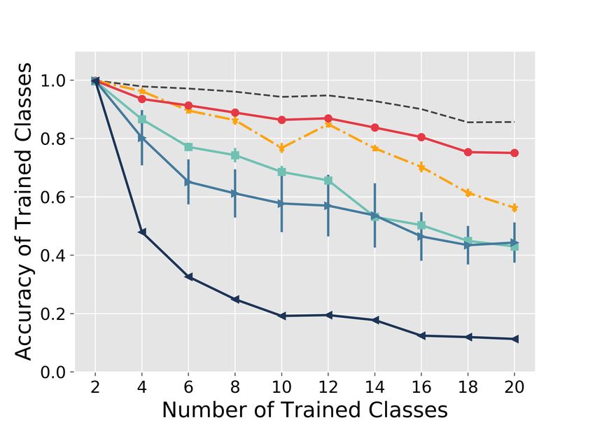
Introduction
Catastrophic forgetting — i.e., when neural networks inadvertently overwrite old memories with
new memories — remains a long-standing problem in machine learning [1]. Here, we studied how
fruit flies learn continuously to associate odors with behaviors and discovered a circuit motif capable
of alleviating catastrophic forgetting.
     While much attention has been paid towards learning good representations for inputs, an equally
challenging problem in continual learning is finding good ways to preserve associations between these
representations and output classes. Indeed, modern deep networks excel at learning complex and
discriminating representations for many data types, which in some cases have resulted in super-
human classification performance [2]. However, these same networks are considerably degraded
when classes are learned sequentially (one at a time), as opposed to being randomly interleaved in
the training data [3–5]. The effect of this simple change is profound and has warranted the search
for new mechanisms that can preserve input-output associations over long periods of time.
     Since learning in the natural world often occurs sequentially, the past few years have wit-
nessed an explosion of brain-inspired continual learning models. These models can be divided into
three categories: 1) regularization models, where important weights (synaptic strengths) are iden-
tified and protected [6–10]; 2) experience replay models, which use external memory to store and
re-activate old data [11], or which use a generative model to generate new data from prior experi-
ence [12–14]; and 3) complementary learning systems [4, 15], which partition memory storage into
multiple sub-networks, each subject to different learning rules and rates. Importantly, these models
often take inspiration from mammalian memory systems, such as the hippocampus [16, 17] or the
neocortex [18, 19], where detailed circuit anatomy and physiology are still lacking. Fortunately,
continual learning is also faced by simpler organisms, such as insects, where supporting circuit
mechanisms are understood at synaptic resolution [20–22].
     Here, we developed an algorithm to reduce catastrophic forgetting by taking inspiration from the
fruit fly olfactory system. This algorithm stitches together three well-known computational ideas
— sparse coding [23–28], synaptic freezing [6–10], and perceptron-style learning [29] — in a unique
and effective way, which we show boosts continual learning performance compared to alternative
algorithms. Importantly, the FlyModel uses neurally-consistent associative learning and does not
require backpropagation. Finally, we show that the fruit fly circuit performs better than alternative
circuits in design space (e.g., replacing sparse coding with dense coding, associative learning with
supervised learning, freezing synapses with not freezing synapses), which provides biological insight
into the function of these evolved circuit motifs and how they operate together in the brain to sustain
memories.

Results
Circuit mechanisms for continual learning in fruit flies
How do fruit flies associate odors (inputs) with behaviors (classes) such that behaviors for odors
learned long ago are not erased by newly learned odors? We first review the basic anatomy and
physiology of two layers of the olfactory system that are relevant to the exposition here. For a more
complete description of this circuit, see Modi et al. [30].
    The two-layer neural circuit we study takes as input an odor after a series of pre-processing
steps have been applied. These steps begin at the sensory layer and include gain control [31, 32],

                                                  2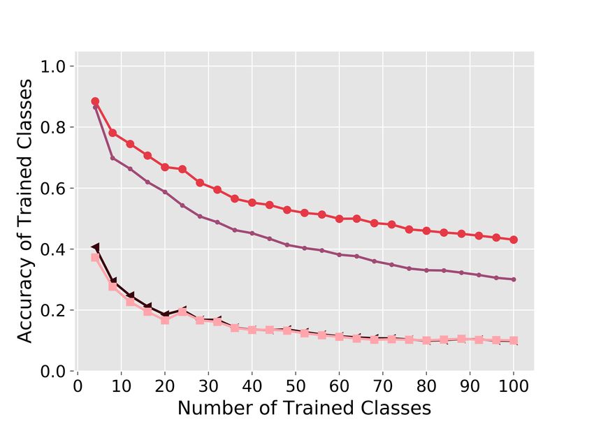
noise reduction [33], and normalization [34, 35]. After these steps, odors are represented by the
firing rates of d = 50 types of projection neurons (PNs), which constitute the input to the two-layer
network motif described next.

Sparse coding. The goal of the first layer is to convert the dense input representation of the PNs
into a sparse, high-dimensional representation [36] (Figure 1A). This is accomplished by a set of
about 2000 Kenyon cells (KCs), which receive input from the PNs. The matrix connecting PNs to
KCs is sparse and approximately random [37]; i.e., each KC randomly samples from about 6 of the 50
projection neurons and sums up their firing rates. Next, each KC provides feed-forward excitation
to a single inhibitory neuron, called APL. In return, APL sends feed-back inhibition to each KC.
The result of this loop is that approximately 95% of the lowest-firing KCs are shut off, and the top
5% remain firing, in what is often referred to as a winner-take-all (WTA) computation [35, 38, 39].
Thus, an odor initially represented as a point in R50+ is transformed, via a 40-fold dimensionality
expansion followed by WTA thresholding, to a point in R2000
                                                          + , where only approximately 100 of the
2000 KCs are active (i.e., non-zero) for any given odor.
    This transformation was previously studied in the context of similarity search [40–43], com-
pressed sensing [35, 44], and pattern separation for subsequent learning [45–47].

Associative learning. The goal of the second layer is to associate odors (sparse points in high-
dimensional space) with behaviors. In the fly, this is accomplished by a set of 34 mushroom body
output neurons (MBONs [48]), which receive input from the 2000 KCs, and then ultimately connect
downstream onto motor neurons that drive behavior. Our focus will be on a subset of MBONs
that encode the learned valence (class) of an odor. For example, there is an “approach” MBON
that strongly responds if the odor was previously associated with a reward, and there is an “avoid”
MBON that responds if the odor was associated with punishment [49]. Thus, the sparse, high-
dimensional odor representation of the KCs is read-out by a smaller set of MBONs that encode
behaviorally-relevant odor information important for decision-making.
    The main locus of associative learning lies at the synapses between KCs and MBONs (Figure 1).
During training, say the fly is presented with a naive odor (odor A) that is paired with a punishment
(e.g., an electric shock). How does the fly learn to avoid odor A in the future? Initially, the synapses
from KCs activated by odor A to both the “approach” MBON and the “avoid” MBON have equal
weights. When odor A is paired with punishment, the KCs representing odor A are activated
around the same time that a punishment-signaling dopamine neuron fires in response to the shock.
The released dopamine causes the synaptic strength between odor A KCs and the approach MBON
to decrease, resulting in a net increase in the avoidance MBON response1 . Eventually, the synaptic
weights between odor A KCs and the approach MBON are sufficiently reduced to reliably learn the
avoidance association [50].
    Importantly, the only synapses that are modified in each associative learning trial are those
from odor A KCs to the approach MBON. All synapses from odor A KCs to the avoid MBON
are frozen (i.e., left unchanged), as are all weights from silent KCs to both MBONs. Thus, the
vast majority of synapses are frozen during any single odor-association trial. How is this imple-
mented biologically? MBONs lie in physically separated “compartments” [48]. Each compartment
has its own dopamine neurons, which only modulate KC→MBON synapses that lie in the same
  1
   Curiously, approach behaviors are learned by decreasing the avoid MBON response, as opposed to increasing the
approach MBON response, as may be more intuitive.

                                                       3
compartment. In the example above, a punishment-signaling dopamine neuron lies in the same
compartment as the approach MBON and only modifies synapses between active KCs and the
approach MBON. Similarly, a reward-signaling dopamine neuron lies in the same compartment
as the avoid MBON [50]. Dopamine released in one compartment does not “spillover” to affect
KC→MBON synapses in neighboring compartments, allowing for compartment-specific learning
rules [51].
To summarize, associative learning in the fly is driven by dopamine signals that only affect the
synapses of sparse odor-activated KCs and a target MBON that drives behavior.
The FlyModel
We now introduce a continual learning algorithm based on the two-layer olfactory circuit described
above.
As input, we are given a d-dimensional vector, x = (x1 , x2 , . . . , xd ) ∈ Rd (analogous to the
projection neuron firing rates for an odor). As in the fly circuit, we assume that x is pre-processed
to remove noise and encode discriminative features. For example, when inputs are images, we could
first pass each image through a deep network and use the representation in the penultimate layer
of the network as input to our two-layer circuit. Pre-processing is essential when the original data
are noisy and not well-separated but could be omitted in simpler datasets with more prominent
separation among classes. To emphasize, our goal here is not to study the complexities of learning
good representations, but rather to develop robust ways to associate inputs with outputs.
The first layer computes a sparse, high-dimensional representation of x. This layer consists of
m units (analogous to Kenyon cells), where m ≈ 40d (analogous to the expansion from 50 PNs to
2000 KCs). The input layer and the first layer are connected by a sparse, binary random matrix,
Θ, of size m × d. Each column of Θ contains about 0.1d ones in random positions (analogous to
each KC sampling from 6 of the 50 PNs), and the rest of the positions in the column are set to
zero. The initial KC representation ψ(x) = (ψ1 , ψ2 , . . . , ψm ) ∈ Rm is computed as:
ψ(x) = Θx. (1)
After this dimensionality expansion, a winner-take-all process is applied, so that only the top l
most active KCs remain on, and the rest of the KCs are set to 0 (in the fly, l = 100, since only 5%
of the 2000 KCs are left active after APL inhibition). This produces a sparse KC representation
φ(x) = (φ1 , φ2 , . . . , φm ) ∈ Rm , where:
(
ψi if ψi is one of the l largest positive entries of ψ(x)
φi = (2)
0 otherwise.
For computational convenience, a min-max normalization is applied to φ(x) so that each KC has a
value between 0 and 1. The matrix Θ is fixed and not modified during learning; i.e., there are no
trainable parameters in the first layer.
The second layer is an associative learning layer, which contains k output class units, y =
{y1 , y2 , . . . , yk } (analogous to MBONs). The m KCs and the k MBONs are connected with all-
to-all synapses. Say an input x is to be associated with target MBON j. When x arrives, a
hypothetical dopamine neuron signaling class j is activated at the same time, so that the only
synapses that are modified are those between the KCs active in φ(x) and the j th MBON. No other
4synapses — including those from the active KCs in φ(x) to the other k − 1 MBONs — are modified.
We refer to this as “partial freezing” of synaptic weights during learning.
Formally, let wij ∈ [0, 1] be the synaptic weight from KC i to MBON j. Then, for all i ∈
[1 . . . m], j ∈ [1 . . . k], the weight update rule after each input x is:
(
(1 − α)wij + βφi if j = target
wij = (3)
(1 − α)wij otherwise.
Here, β is the learning rate, and α is a very small forgetting term that mimics slow, background
memory decay. In our experiments, we set α = 0 to minimize forgetting and to simplify the model.
The problem of weight saturation arises when α = 0, since weights can only increase, and never
decrease. However, despite tens of thousands of training steps, the vast majority of weights did
not saturate since most KCs are inactive for most classes (sparse coding) and only a small fraction
of the active KC synapses are modified during learning (partial freezing). Nonetheless, in practice,
some small, non-zero α may be desired to avoid every synapse from eventually saturating.
Finally, biological synaptic weights have physical bounds on their strength, and here we mimic
these bounds by capping weights to [0, 1].
Similarities and differences to the fruit fly olfactory circuit. The FlyModel is based on two
core features of the fruit fly olfactory circuit: sparse coding and partial freezing of synaptic weights
during learning. There are, however, additional complexities of this “two-layer” olfactory circuit
that we do not consider here. First, there are additional recurrent connections in the circuit,
including KC↔KC connections [52] and dopamine↔MBON connections [20, 53]; further, there
is an extensive, four-layer network of interactions amongst MBONs [48], the function of which
still remains largely unknown. Second, we assume KCs and MBONs make all-to-all connections,
whereas in reality, each MBON is typically connected to less than half of the KCs. KCs are
divided into distinct lobes that innervate different compartments [48]. Lobes and compartments
allow for an odor’s KC representation to be “split” into a parallel memory architecture, where
each compartment has a different memory storage capacity, update flexibility, and retention and
decay rates [51]. Third, we assumed that co-activation of dopamine neurons and KCs increases
the synaptic weights between KCs and the target MBON, whereas in reality, when learning to
avoid an odor, the strength of response to the opposite behavior (approach MBON) is decreased.
Conceptually, the net effect is equivalent for binary classification, but the latter leads to additional
weight interference when there are > 2 classes because it requires decreasing weights to all non-
target MBONs.
We excluded these additional features to reduce the number of model parameters and to sharpen
our focus on the two core features mentioned above. These abstractions are in line with those
made by previous models of this circuit (e.g. [35, 54, 55]). Some of these additional features may
be useful in more sophisticated continual learning problems that are beyond the scope of our work
here (Discussion).
Testing framework and problem setup
We tested each algorithm on two datasets using a class-incremental learning setup [12, 56], in
which the training data was ordered and split into sequential tasks. For the MNIST-20 dataset
(a combination of regular MNIST and Fashion MNIST; Methods), we used 10 non-overlapping
5tasks, where each task is a classification problem between two classes. For example, the first task
is to classify between digits 0 and 1, the second task is to classify digits 2 and 3, etc. Similarly,
the CIFAR-100 dataset (Methods) is divided into 25 non-overlapping tasks, where each task is a
classification problem among four classes. In each task, all instances of one class are presented
sequentially, followed by all instances of the second class. Only a single pass is made through the
training data (i.e., one epoch) to mimic an online learning problem.
Testing is performed after the completion of training of each task, and is quantified using two
measures. The first measure — the accuracy for classes trained so far — assesses how well classes
from previous tasks remain correctly classified after a new task is learned. Specifically, after train-
ing task i, we report the accuracy of the model when tested on classes from all tasks ≤ i. For
example, say a model has been trained on the first three tasks — classify 0 vs. 1, 2 vs. 3, and 4 vs.
5. During the test phase of task three, the model is presented with test examples from digits 0–5,
and their accuracy is reported. The second measure — memory loss — quantifies forgetting for
each task separately. We define the memory loss of task i as the accuracy of the model when tested
(on classes from task i only) immediately after training on task i minus the accuracy when tested
(again, on classes from task i only) after training on all tasks, i.e., at the end of the experiment.
For example, say the immediate accuracy of task i is 0.80, and the accuracy of task i at the end of
the experiment is 0.70. Then the memory loss of task i is 0.10. A memory loss of zero means that
the memory of the task was perfectly preserved despite learning new tasks.
Comparison to other methods. We compared the FlyModel with five methods, briefly described
below:
1. Elastic weight consolidation (EWC [9]) uses the Fisher information criterion to identify
weights that are important for previously learned tasks, and then introduces a penalty if
these weights are modified when learning a new task.
2. Gradient episodic memory (GEM [11]) uses a memory system that stores a subset of data
from previously learned tasks. These data are used to assess how much the loss function on
previous tasks increases when model parameters are updated for a new task.
3. Brain-inspired replay (BI-R [12]) protects old memories by using a generative model to replay
activity patterns related to previously learned tasks. The replayed patterns are generated
using feedback connections, without storing data.
4. Vanilla is a standard fully-connected neural network that does not have any explicit continual
learning mechanism. This is used as a lower bound on performance.
5. Offline is a standard fully-connected neural network, but instead of learning tasks sequentially,
it is presented with all classes from the tasks in a random order. For example, for the third
task on MNIST-20, Offline is trained with digits 0–5 randomly shuffled. Then, for the fourth
task, Offline is re-trained from scratch on digits 0–7. The Offline model is used as an upper
bound on performance.
All five of these methods use backpropagation for training weights (both PN→KC weights and
KC→MBON weights). In addition, all five methods (except BI-R; Methods) use the same archi-
tecture as the FlyModel— the same number of layers, the same number of units per layer (m KCs
6in the first layer, k MBONs in the second layer) — and they all use the same hidden unit activa-
tion function (ReLU). Finally, for a fair comparison, all methods, including the FlyModel, use the
same representation for each input. Thus, the primary difference amongst methods is how learning
mechanisms store and preserve memories.
The FlyModel outperforms existing methods in class-incremental learning
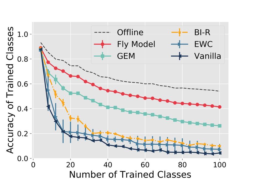
The FlyModel reduced catastrophic forgetting compared to all four continual learning methods
tested. For example, on the MNIST-20 dataset (Figure 2A), after training on 5 tasks (10 classes),
the accuracy of the FlyModel was 0.86 ± 0.0006 compared to 0.77 ± 0.02 for BI-R, 0.69 ± 0.02 for
GEM, 0.58 ± 0.10 for EWC, and 0.19 ± 0.0003 for Vanilla. At the end of training (10 tasks, 20
classes trained), the test accuracy of the FlyModel was at least 0.19 higher than any other method,
and only 0.11 lower than the optimal Offline model, which is trained using all classes presented
together, instead of sequentially.
Next, we used the memory loss measure (Methods) to quantify how well the “memory” of an
old task is preserved after training new tasks (Figure 2B, Figure S1). As expected, the standard
neural network (Vanilla) preserves almost no memory of previous tasks; i.e., it has a memory loss
of nearly 1 for all tasks except the most recent task. While GEM, EWC, and BI-R perform better
— memory losses of 0.24, 0.27, and 0.42, respectively, averaged across all tasks — the FlyModel
has an average memory loss of only 0.07. This means that the accuracy of task i was only degraded
on average by 7% at the end of training when using the FlyModel.
Similar trends were observed on a second, more difficult dataset (CIFAR-100; Figure 2C–D),
where the FlyModel had an accuracy that was at least 0.15 greater than all continual learning
methods, and performed only 0.13 worse than the Offline model.
Sparse coding and partial freezing are both required for continual learning
An important challenge in theoretical neuroscience is to understand why circuits may be designed
the way they are. Quantifying how evolved circuits fare against putative, alternative circuits in
design space could provide insight into the biological function of observed network motifs. We first
explored this question in the context of the two core components in the FlyModel: sparse coding of
representations in the first layer, and partial freezing of synaptic weights in the associative learning
layer. Are both of these components required, or can good performance be attained with only one
or the other?
We piecemeal explored the effects of replacing sparse coding with dense coding, and replacing
partial freezing with a traditional single layer neural network (i.e., logistic regression), where every
weight can change for each input. This gave us four combinations to test. The dense code was
calculated in the same way as the sparse code, minus the winner-take-all step. In other words,
for each input x, we used ψ(x) (Equation (1), with min-max normalization) as its representation,
instead of φ(x) (Equation (2)). For logistic regression, the associative layer was trained using
backpropagation.
Both sparse coding variants (with partial freezing or with logistic regression) performed sub-
stantially better than the two dense coding variants on both datasets (Figure 3A–B). For example,
on MNIST-20, at the end of training, the sparse coding models had an average accuracy of 0.64
compared to 0.07 for the two dense coding models. Further, sparse coding with partial freezing
7(i.e., the FlyModel) performed better than sparse coding with logistic regression: 0.75 vs. 0.54 on
MNIST-20; 0.41 vs. 0.21 on CIFAR-100.
Hence, on at least the two datasets used here, both sparse coding and partial freezing are needed
to optimize continual learning performance.
Empirical and theoretical comparison of the FlyModel with the perceptron
The fruit fly associative learning algorithm (partial freezing) bears resemblance to a well-known
supervised learning algorithm — the perceptron [57] — albeit two differences. First, both algo-
rithms increase weights to the correct target MBON (class), but the perceptron also decreases the
weights to the incorrect MBON if a mistake is made. Second, the perceptron does not modify
weights when a correct prediction is made, whereas partial freezing updates weights even if the
correct prediction is made. Next, we continued our exploration of circuit design space by studying
how the four combinations of these two rules affect continual learning.
The first model (Perceptron v1) is the classic perceptron learning algorithm, where weights are
only modified if an incorrect prediction is made, by increasing weights to the correct class and
decreasing weights to the incorrectly predicted class. The second model (Perceptron v2) also only
learns when a mistake is made, but it only increases weights to the correct class (i.e., it does not
decrease weights to the incorrect class). The third model (Perceptron v3) increases weights to the
correct class regardless of whether a mistake is made, and it decreases weights to the incorrect class
when a mistake is made. Finally, the fourth model (Perceptron v4) is equivalent to the FlyModel;
it simply increases weights to the correct class regardless of whether a mistake is made. All models
start with the same sparse, high-dimensional input representations in the first layer. See Methods
for pseudocode for each model.
Overall, we find a striking difference in continual learning with these two tweaks, with the
FlyModel performing significantly better than the other three models on both datasets (Figure 4A–
B). Specifically, learning regardless of whether a mistake is made (v3 and v4) works better than
mistake-only learning (v1 and v2), and decreasing the weights to incorrectly predicted class hurts
performance (v4 compared to v3; no major difference between v2 and v1).
Why does decreasing weights to the incorrect class (v1 and v3) result in poor performance? This
feature of the perceptron algorithm is believed to help create a larger boundary (margin) between
the predicted incorrect class and the correct class. However, in the Supplement (Lemma 2), we
show analytically that under continual learning, it is easy to come up with instances where this
feature leads to catastrophic forgetting. Intuitively, this occurs when two (similar) inputs share
overlapping representations, yet belong to different classes. The synapses of shared neurons are
strengthened towards the the class most recently observed, and weakened towards the other class.
Thus, when the first input is observed again, it is associated with the second input’s class. In
other words, decreasing weights to the incorrect class causes shared weights to be “hijacked” by
recent classes observed (Figure S2A–C). We tested this empirically on the MNIST-20 dataset and
found that, while decreasing weights when mistakes are made enables faster initial discrimination,
it also leads to faster forgetting (Figure S3A). Indeed, this effect is particularly pronounced when
the two classes are similar (digits ‘3’ vs. ‘5’; Figure S3B) rather than dissimilar (digits ‘3’ vs. ‘4’;
Figure S3C). In contrast, the FlyModel avoids this issue because the shared neurons are “split”
between both classes, and thus, cancel each other out (Figure S2D, Figure S3).
In support of our empirical findings, we show analytically that partial freezing in the FlyModel
(v4) reduces catastrophic forgetting because MBON weight vectors converge over time to the mean
8of its class inputs scaled by a constant (Supplement, Lemmas 3 and 4, Theorems 5 and 8).
Sparse coding provably creates favorable separation for continual learning
Why does sparse coding reduce memory interference under continual learning? We first show that
the partial freezing algorithm alone will provably learn to correctly distinguish classes if the classes
satisfy a separation condition that says, roughly, that dot products between points within the
same class are, on average, greater than between classes. We then show that adding sparse coding
enhances the separation of classes [45], making associative learning easier.
Definition 1. Let π1 , . . . , πk be distributions over Rd , corresponding to k classes of data points.
We say the classes are γ-separated, for some γ > 0, if for any pair of classes j 6= j 0 , and any point
xo from class j,
EX∼πj [xo · X] ≥ γ + EX 0 ∼πj 0 [xo · X 0 ].
Here, the notation EX∼π refers to expected value under a vector X drawn at random from distri-
bution π.
Under γ-separation, the labeling rule
x 7→ arg max wj · x
j
is a perfect classifier if the wj (i.e., the KC → MBON weight vector for class j) are the means of their
respective classes, that is, wj = EX∼πj [X]. This holds even if the means are only approximately
accurate, within O(γ) (Supplement, Theorem 8). The partial freezing algorithm can, in turn, be
shown to produce such mean-estimates (Supplement, Theorem 5).
The separation condition of Definition 1 is quite strong and might not hold in the original data
space. But we will show that subsequent sparse coding can nonetheless produce this condition, so
that the partial freezing algorithm, when run on the sparse encodings, performs well.
To see a simple model of how this can happen, suppose that there are N prototypical inputs,
denoted p1 , . . . , pN ∈ X , where X ⊂ Rd , that are somewhat separated from each other:
pi · pj
≤ ξ,
kpi kkpj k
for some ξ ∈ [0, 1). Each pi has a label yi ∈ {1, 2, . . . , k}. Let Cj ⊂ [N ] be the set of prototypes
whose label is j. Since the labels are arbitrary, these classes will in general not be linearly separable
in the original space (Figure S4).
Suppose the sparse coding map φ : X → {0, 1}m generates k-sparse representations with the
following property: for any x, x0 ∈ X ,
x · x0
0
φ(x) · φ(x ) ≤ k f ,
kxkkx0 k
where f : [−1, 1] → [0, 1] is a function that captures how the coding process transforms dot products.
In earlier work [41], we have characterized f for two types of random mappings, a sparse binary
matrix (inspired by the fly’s architecture) and a dense Gaussian matrix (common in engineering
applications). In either case, f (s) is a much shrunken version of s; in the dense Gaussian case, for
instance, it is roughly (k/m)1−s .
9We can show that for suitable ξ, the sparse representations of the prototypes — that is,
φ(p1 ), . . . , φ(pN ) ∈ {0, 1}m — are then guaranteed to be separable, so that the partial freezing
algorithm will converge to a perfect classifier.
Theorem 2. Let No = maxj |Cj |. Under the assumptions above, the sparse representation of the
data set, {(φ(p1 ), y1 ), . . . , (φ(pN ), yN )}, is (1/No − f (ξ))-separated in the sense of Definition 1.
Proof. This is a consequence of Theorem 9 in the Supplement, a more general result that applies
to a broader model in which observed data are noisy versions of the prototypes.
Discussion
We developed a simple and light-weight neural algorithm to alleviate catastrophic forgetting, in-
spired by how fruit flies learn odor-behavior associations. The FlyModel outperformed three popu-
lar class-incremental continual learning algorithms on two benchmark datasets (MNIST-20 and
CIFAR-100), despite not using external memory, generative replay, nor backpropagation. We
showed that alternative circuits in design space, including the classic perceptron learning rule,
suffered more catastrophic forgetting than the FlyModel, potentially shedding new light on the
biological function and conservation of this circuit motif. Finally, we grounded these ideas theoreti-
cally by proving that MBON weight vectors in the FlyModel converge to the mean representation of
its class, and that sparse coding further reduces memory interference by better separating classes.
Our work exemplifies how understanding detailed neural anatomy and physiology in a tractable
model system can be translated into efficient architectures for use in artificial neural networks.
The two main features of the FlyModel— sparse coding and partial synaptic freezing — are
well-appreciated in both neuroscience and machine learning. For example, sparse, high-dimensional
representations have long been recognized as central to neural encoding [58], hyper-dimensional
computing [59], and classification and recognition tasks [45]. However, the benefits of such rep-
resentations towards continual learning have not been well-quantified. Similarly, the notion of
“freezing” certain weights during learning has been used in both classic perceptrons and modern
deep networks [9, 10], but these methods are still subject to interference caused by dense repre-
sentations. Hence, the fruit fly circuit evolved a unique combination of common computational
ingredients that work effectively in practice.
The FlyModel performs associative rather than supervised learning. In associative learning,
the same learning rule is applied regardless of whether the model makes a mistake. In traditional
supervised learning, changes are only made to weights when the model makes a mistake, and the
changes are applied to weights for both the correct and the incorrect class labels. By performing
associative learning, the FlyModel garners two benefits. First, the FlyModel learns each class
independently compared to supervised methods, which focus on discrimination between multiple
classes at a time. We showed that the latter is particularly susceptible to interference, especially
when class representations are overlapping. Second, by learning each class independently, the
FlyModel is flexible about the total number of classes to be learned; the network is easily expandable
to more classes, if necessary. Our results suggest that some traditional benefits of supervised
classification may not carry over into the continual learning setting [60], and that association-like
models may better preserve memories when classes are learned sequentially.
There are additional features of the fruit fly circuitry (specifically, the mushroom body) that
remain under-explored computationally. First, instead of using one output neuron (MBON) per
10behavior, the mushroom body contains multiple output neurons per behavior, with each output
neuron learning at a different rate [49, 51]. This simultaneously provides fast learning with poor
retention (large learning rates) and slow learning with longer retention (small learning rates),
which is reminiscent of complementary learning systems [1]. Second, the mushroom body contains
mechanisms for memory extinction [50] and reversal learning [61, 62], which are used to over-write
specific memories that are no longer accurate. Third, there is evidence of memory replay in the
mushroom bodytriggered by a neuron called DPM, which is required not during, but rather after
memory formation, in order for memories to be consolidated [63–65].
Beyond catastrophic forgetting, there are additional challenges of continual learning that remain
outstanding. These challenges include forward transfer learning (i.e., information learned in the
past should help with learning new information more efficiently) and backward transfer learning
(i.e., learning new information helps “deepen” the understanding of previously learned information).
None of the algorithms we tested, including the FlyModel, were specifically designed to addresses
these challenges, with the exception of GEM [11], which indeed achieved slightly negative memory
losses (i.e., tasks learned after task i improve the accuracy of task i; Figure 2D), indicating some
success at backward transfer learning. Biologically, circuit mechanisms supporting transfer learning
remain unknown.
Finally, a motif similar to that of the fruit fly olfactory system also appears in the mouse
olfactory system, where sparse representations in the piriform cortex project to other learning-
related areas of the brain [66, 67]. In addition, the visual system uses many successive layers
to extract discriminative features [68, 69], which are then projected to the hippocampus, where
a similar sparse, high-dimensional representation is used for memory storage [70–72]. Thus, the
principles of learning studied here may help illuminate how continual learning is implemented in
other brain regions and species.
Methods
Datasets and pre-processing We tested our model on two datasets.
MNIST-20: This benchmark combines MNIST and Fashion MNIST. For training, MNIST
contains 60,000 gray-scale images of 10 classes of hand-written digits (0–9), and Fashion MNIST [73]
contains 60,000 gray-scale images of 10 classes of fashion items (e.g., purse, pants, etc.). The test
set contains 10,000 additional images from each dataset. Together, the two datasets contain 20
classes. The 10 digits in MNIST are labelled 0–9, and the 10 classes in Fashion MNIST are labelled
10–19 in our experiments. To generate a generic input representation for each image, we trained
a LeNet5 [74] network (learning rate = 0.001, batch size = 64, number of epochs = 25, with
batch normalization and Adam) on KMNIST [75], which contains 60,000 images for 10 classes of
hand-written Japanese characters. The penultimate layer of this network contains 84 hidden units
(features). We used this trained LeNet5 as an encoder to extract 84 features for each training and
test image in MNIST and Fashion MNIST.
CIFAR-100: This benchmark contains 50,000 RGB images for 100 classes of real-life objects
in the training set, and 10,000 images in the testing set. To generate input representations, we
used the penultimate layer (512 hidden nodes) of ResNet18 [76] pre-trained on ImageNet (down-
loaded from https://pytorch.org/docs/stable/torchvision/models.html#id27). Thus, each
CIFAR-100 image was represented as a 512-dimensional vector.
11Network architectures. All methods we tested share the same network architecture: a three-
layer network with an input layer (analog to PNs in fruit flies), a single hidden layer (analog to KCs)
and an output layer (analog to the MBONs). For the MNIST-20 dataset, the network contains 84
nodes in the input layer, 3200 nodes in the hidden layer, and 20 nodes in the output layer. For
CIFAR-100, these three numbers are 512, 20000, and 100 respectively. The size of the hidden layer
was selected to be approximately 40x larger than the input layer, as per the fly circuit.
For all models except the FlyModel, the three layers make all-to-all connections. For fly model,
the PN and KC layer are connected via a sparse random matrix (Θ); each KC sums over 10 ran-
domly selected PNs for MNIST-20, and 64 randomy PNs for CIFAR-100.
Implemenations of other methods. GEM and EWC implementations are adapted from:
https://github.com/facebookresearch/GradientEpisodicMemory. The BI-R implementation
is adapted from: https://github.com/GMvandeVen/brain-inspired-replay.
Parameters. Parameters for each model and dataset were independently selected using grid search
to maximize accuracy.
• FlyModel: learning rate: 0.01 (MNIST-20), 0.2 (CIFAR-100); l = m/k, where k = 20, the
number of classes for MNIST-20 and k = 100 for CIFAR-100; and m = 3200, the number of
Kenyon cells for MNIST-20, and m = 20000 for CIFAR-100.
• GEM: learning rate: 0.001, memory strength: 0.5, n memories: 256, batch size: 64, for both
datasets.
• EWC: learning rate: 0.1 (MNIST-20), 0.001 (CIFAR-100); memory strength: 1000, n memo-
ries: 1000, batch size: 64, for both datasets.
• BI-R: learning rate: 0.001, batch size: 64 for both datasets. The BI-R architecture and other
parameters are default to the original implementation [12].
• Vanilla: learning rate: 0.001, batch size: 64, for both datasets.
• Offline: learning rate: 0.001, batch size: 64, for both datasets.
For Offline, Vanilla, EWC, and GEM, a softmax activation is used for the output layer, and op-
timization is performed using stochasic gradient descent (SGD). For BI-R, no activation function is
applied to the output layer, and optimization is performed using Adam with β1 = 0.900, β2 = 0.999.
We report the average and standard deviation of both evaluation measures for each method
over five random initializations.
12Perceptron variations. The update rules for the four perceptron variations are listed below:
Perceptron v1 (Original) Perceptron v2
1: for x in data do 1: for x in data do
2: if predict 6= target then 2: if predict 6= target then
3: weight[target] += βx 3: weight[target] += βx
4: weight[predict] −= βx 4:
5: end if 5: end if
6: end for 6: end for
Perceptron v3 Perceptron v4 (FlyModel)
1: for x in data do 1: for x in data do
2: if predict 6= target then 2: if predict 6= target then
3: weight[target] += βx 3: weight[target] += βx
4: weight[predict] −= βx 4:
5: else 5: else
6: weight[target] += βx 6: weight[target] += βx
7: end if 7: end if
8: end for 8: end for
13Figures
A B
random
projection
…
…
deep network
Projection Kenyon cells (KCs) MBONs
neurons (PNs) frozen modified
input layer sparse, high-dimensional output
representation classes
Figure 1: A two-layer circuit for continual learning in the fruit fly olfactory system. A)
An input (odor) is received by the sensory layer and pre-processed via a series of transformations.
In the fruit fly, this pre-processing includes noise reduction, normalization, and gain control. In
a deep network, pre-processing is similarly used to generate a suitable representation for learning.
After these transformations, the dimensionality of the pre-processed input (PNs) is expanded via
a random projection and is sparsified via winner-take-all thresholding. This leaves only a few
Kenyon cells active per odor (indicated by red shading). To associate the odor with an output class
(MBON), only the synapses connecting the active Kenyon cells to the target MBON are modified.
The rest of the synapses are frozen. B) A second example with a second odor, showing different
Kenyon cells activated, associated with a different MBON.
14A B
MNIST-20
C D
CIFAR-100
Figure 2: The FlyModel outperforms existing continual learning methods in class-
incremental learning. A) The x-axis is the number of classes trained on, and the y-axis is
the classification accuracy when testing the model on the classes trained on thus far. The Offline
method (dashed black line) shows the optimal classification accuracy when classes are presented
together, instead of sequentially. Error bars show standard deviation of the test accuracy over 5
random initializations for GEM, BI-R, EWC, and Vanilla, or over 5 random matrices (Θ) for the
FlyModel. B) The x-axis is the task number during training, and the y-axis is the memory loss
of the task, which measures how much the network has forgotten about the task as a result of
subsequent training. A–B) MNIST-20 dataset. C–D) CIFAR-100. The memory loss of all tasks is
shown in Figure S1.
15A MNIST-20 B CIFAR-100
Figure 3: Sparse coding and partial freezing are both required for continual learning.
Axes are the same as those in Figure 2A. Both sparse coding methods outperform both dense coding
methods. When using sparse coding, partial freezing outperforms logistic regression (1-layer neural
network). A) MNIST-20. B) CIFAR-100.
A MNIST-20 B CIFAR-100
Figure 4: Continual learning performance for the four perceptron variants. Axes are the
same as those in Figure 2A. Compared to the classic perceptron learning algorithm (Perceptron
v1), the FlyModel (Perceptron v4) learns regardless of whether a mistake is made, and it does not
decrease weights to the incorrect class when mistakes are made. These two changes significantly
improve continual learning performance. A) MNIST-20. B) CIFAR-100.
16References
[1] Parisi, G. I., Kemker, R., Part, J. L., et al. “Continual lifelong learning with neural networks:
A review”. Neural Netw 113 (2019), pp. 54–71.
[2] LeCun, Y., Bengio, Y., and Hinton, G. “Deep learning”. Nature 521.7553 (2015), pp. 436–444.
[3] Ratcliff, R. “Connectionist models of recognition memory: constraints imposed by learning
and forgetting functions”. Psychol Rev 97.2 (1990), pp. 285–308.
[4] McClelland, J. L., McNaughton, B. L., and O’Reilly, R. C. “Why there are complementary
learning systems in the hippocampus and neocortex: insights from the successes and failures
of connectionist models of learning and memory”. Psychol Rev 102.3 (1995), pp. 419–457.
[5] French, R. M. “Catastrophic forgetting in connectionist networks”. Trends Cogn Sci 3.4
(1999), pp. 128–135.
[6] Hinton, G. E. and Plaut, D. C. “Using Fast Weights to Deblur Old Memories”. Proc. of the
9th Annual Conf. of the Cognitive Science Society. Erlbaum, 1987, pp. 177–186.
[7] Fusi, S., Drew, P. J., and Abbott, L. F. “Cascade models of synaptically stored memories”.
Neuron 45.4 (2005), pp. 599–611.
[8] Benna, M. K. and Fusi, S. “Computational principles of synaptic memory consolidation”. Nat
Neurosci 19.12 (Dec. 2016), pp. 1697–1706.
[9] Kirkpatrick, J., Pascanu, R., Rabinowitz, N., et al. “Overcoming catastrophic forgetting in
neural networks”. Proc Natl Acad Sci U S A 114.13 (Mar. 2017), pp. 3521–3526.
[10] Zenke, F., Poole, B., and Ganguli, S. “Continual Learning Through Synaptic Intelligence”.
Proc Mach Learn Res 70 (2017), pp. 3987–3995.
[11] Lopez-Paz, D. and Ranzato, M. “Gradient episodic memory for continual learning”. Advances
in neural information processing systems. 2017, pp. 6467–6476.
[12] Ven, G. M. van de, Siegelmann, H. T., and Tolias, A. S. “Brain-inspired replay for continual
learning with artificial neural networks”. Nat Commun 11.1 (Aug. 2020), p. 4069.
[13] Tadros, T., Krishnan, G. P., Ramyaa, R., and Bazhenov, M. “Biologically Inspired Sleep
Algorithm for Reducing Catastrophic Forgetting in Neural Networks”. The Thirty-Fourth
AAAI Conference on Artificial Intelligence, AAAI, New York, NY, USA. AAAI Press, 2020,
pp. 13933–13934.
[14] Shin, H., Lee, J. K., Kim, J., and Kim, J. “Continual learning with deep generative replay”.
arXiv preprint arXiv:1705.08690v3 (2017).
[15] Roxin, A. and Fusi, S. “Efficient partitioning of memory systems and its importance for
memory consolidation”. PLoS Comput Biol 9.7 (2013), e1003146.
[16] Wilson, M. A. and McNaughton, B. L. “Reactivation of hippocampal ensemble memories
during sleep”. Science 265.5172 (1994), pp. 676–679.
[17] Rasch, B. and Born, J. “Maintaining memories by reactivation”. Curr Opin Neurobiol 17.6
(2007), pp. 698–703.
[18] Qin, Y. L., McNaughton, B. L., Skaggs, W. E., and Barnes, C. A. “Memory reprocessing
in corticocortical and hippocampocortical neuronal ensembles”. Philos Trans R Soc Lond B
Biol Sci 352.1360 (1997), pp. 1525–1533.
17[19] Ji, D. and Wilson, M. A. “Coordinated memory replay in the visual cortex and hippocampus
during sleep”. Nat Neurosci 10.1 (2007), pp. 100–107.
[20] Takemura, S. Y., Aso, Y., Hige, T., et al. “A connectome of a learning and memory center
in the adult Drosophila brain”. Elife 6 (July 2017).
[21] Zheng, Z., Lauritzen, J. S., Perlman, E., et al. “A Complete Electron Microscopy Volume of
the Brain of Adult Drosophila melanogaster”. Cell 174.3 (July 2018), pp. 730–743.
[22] Li, F., Lindsey, J. W., Marin, E. C., et al. “The connectome of the adult Drosophila mushroom
body provides insights into function”. Elife 9 (2020).
[23] Maurer, A., Pontil, M., and Romera-Paredes, B. “Sparse Coding for Multitask and Transfer
Learning”. Proc. 30th Intl. Conf. on Machine Learning - Volume 28. ICML’13. Atlanta, GA,
USA: JMLR.org, 2013, II–343–II–351.
[24] Ruvolo, P. and Eaton, E. “ELLA: An Efficient Lifelong Learning Algorithm”. Proceedings of
the 30th International Conference on Machine Learning. Ed. by Dasgupta, S. and McAllester,
D. Vol. 28. Proceedings of Machine Learning Research 1. Atlanta, Georgia, USA: PMLR, 2013,
pp. 507–515.
[25] Ororbia, A., Mali, A., Kifer, D., and Giles, C. L. “Lifelong Neural Predictive Coding: Sparsity
Yields Less Forgetting when Learning Cumulatively”. CoRR abs/1905.10696 (2019). arXiv:
1905.10696.
[26] Ahmad, S. and Scheinkman, L. “How Can We Be So Dense? The Benefits of Using Highly
Sparse Representations”. CoRR abs/1903.11257 (2019). arXiv: 1903.11257.
[27] Rapp, H. and Nawrot, M. P. “A spiking neural program for sensorimotor control during
foraging in flying insects”. Proc Natl Acad Sci U S A 117.45 (Nov. 2020), pp. 28412–28421.
[28] Hitron, Y., Lynch, N., Musco, C., and Parter, M. “Random Sketching, Clustering, and
Short-Term Memory in Spiking Neural Networks”. 11th Innovations in Theoretical Computer
Science Conference (ITCS 2020). Ed. by Vidick, T. Vol. 151. Dagstuhl, Germany: Schloss
Dagstuhl–Leibniz-Zentrum fuer Informatik, 2020, 23:1–23:31.
[29] Minsky, M. L. and Papert, S. A. Perceptrons: Expanded Edition. Cambridge, MA, USA: MIT
Press, 1988.
[30] Modi, M. N., Shuai, Y., and Turner, G. C. “The Drosophila Mushroom Body: From Archi-
tecture to Algorithm in a Learning Circuit”. Annu Rev Neurosci 43 (July 2020), pp. 465–
484.
[31] Root, C. M., Masuyama, K., Green, D. S., et al. “A presynaptic gain control mechanism
fine-tunes olfactory behavior”. Neuron 59.2 (2008), pp. 311–321.
[32] Gorur-Shandilya, S., Demir, M., Long, J., et al. “Olfactory receptor neurons use gain control
and complementary kinetics to encode intermittent odorant stimuli”. Elife 6 (June 2017).
[33] Wilson, R. I. “Early olfactory processing in Drosophila: mechanisms and principles”. Annu
Rev Neurosci 36 (2013), pp. 217–241.
[34] Olsen, S. R., Bhandawat, V., and Wilson, R. I. “Divisive normalization in olfactory population
codes”. Neuron 66.2 (2010), pp. 287–299.
[35] Stevens, C. F. “What the fly’s nose tells the fly’s brain”. Proc Natl Acad Sci U S A 112.30
(2015), pp. 9460–9465.
18[36] Cayco-Gajic, N. A. and Silver, R. A. “Re-evaluating Circuit Mechanisms Underlying Pattern
Separation”. Neuron 101.4 (Feb. 2019), pp. 584–602.
[37] Caron, S. J., Ruta, V., Abbott, L., and Axel, R. “Random convergence of olfactory inputs in
the Drosophila mushroom body”. Nature 497.7447 (2013), pp. 113–117.
[38] Turner, G. C., Bazhenov, M., and Laurent, G. “Olfactory representations by Drosophila
mushroom body neurons”. J Neurophysiol 99.2 (2008), pp. 734–746.
[39] Lin, A. C., Bygrave, A. M., Calignon, A. de, et al. “Sparse, decorrelated odor coding in the
mushroom body enhances learned odor discrimination”. Nat Neurosci 17.4 (2014), pp. 559–
568.
[40] Dasgupta, S., Stevens, C. F., and Navlakha, S. “A neural algorithm for a fundamental com-
puting problem”. Science 358.6364 (Nov. 2017), pp. 793–796.
[41] Dasgupta, S., Sheehan, T. C., Stevens, C. F., and Navlakha, S. “A neural data structure for
novelty detection”. Proc Natl Acad Sci U S A 115.51 (Dec. 2018), pp. 13093–13098.
[42] Papadimitriou, C. H. and Vempala, S. S. “Random Projection in the Brain and Computation
with Assemblies of Neurons”. 10th Innovations in Theoretical Computer Science Conference
(ITCS 2019). Ed. by Blum, A. Vol. 124. Leibniz International Proceedings in Informatics
(LIPIcs). Dagstuhl, Germany: Schloss Dagstuhl–Leibniz-Zentrum fuer Informatik, 2018, 57:1–
57:19.
[43] Ryali, C., Hopfield, J., Grinberg, L., and Krotov, D. “Bio-Inspired Hashing for Unsupervised
Similarity Search”. Proceedings of the 37th International Conference on Machine Learning.
Ed. by III, H. D. and Singh, A. Vol. 119. Proceedings of Machine Learning Research. PMLR,
2020, pp. 8295–8306.
[44] Zhang, Y. and Sharpee, T. O. “A Robust Feedforward Model of the Olfactory System”. PLoS
Comput Biol 12.4 (2016), e1004850.
[45] Babadi, B. and Sompolinsky, H. “Sparseness and expansion in sensory representations”. Neu-
ron 83.5 (2014), pp. 1213–1226.
[46] Litwin-Kumar, A., Harris, K. D., Axel, R., et al. “Optimal Degrees of Synaptic Connectivity”.
Neuron 93.5 (2017), pp. 1153–1164.
[47] Dasgupta, S. and Tosh, C. Expressivity of expand-and-sparsify representations. 2020. arXiv:
2006.03741 [cs.NE].
[48] Aso, Y., Hattori, D., Yu, Y., et al. “The neuronal architecture of the mushroom body provides
a logic for associative learning”. elife 3 (2014), e04577.
[49] Hige, T., Aso, Y., Modi, M. N., et al. “Heterosynaptic Plasticity Underlies Aversive Olfactory
Learning in Drosophila”. Neuron 88.5 (2015), pp. 985–998.
[50] Felsenberg, J., Jacob, P. F., Walker, T., et al. “Integration of Parallel Opposing Memories
Underlies Memory Extinction”. Cell 175.3 (Oct. 2018), pp. 709–722.
[51] Aso, Y. and Rubin, G. M. “Dopaminergic neurons write and update memories with cell-type-
specific rules”. Elife 5 (July 2016).
[52] Eichler, K., Li, F., Litwin-Kumar, A., et al. “The complete connectome of a learning and
memory centre in an insect brain”. Nature 548.7666 (Aug. 2017), pp. 175–182.
19[53] Cervantes-Sandoval, I., Phan, A., Chakraborty, M., and Davis, R. L. “Reciprocal synapses
between mushroom body and dopamine neurons form a positive feedback loop required for
learning”. Elife 6 (May 2017).
[54] Peng, F. and Chittka, L. “A Simple Computational Model of the Bee Mushroom Body Can
Explain Seemingly Complex Forms of Olfactory Learning and Memory”. Curr Biol 27.11
(June 2017), p. 1706.
[55] Mittal, A. M., Gupta, D., Singh, A., et al. “Multiple network properties overcome random
connectivity to enable stereotypic sensory responses”. Nat Commun 11.1 (Feb. 2020), p. 1023.
[56] Farquhar, S. and Gal, Y. “Towards robust evaluations of continual learning”. arXiv preprint
arXiv:1805.09733v3 (2019).
[57] Rosenblatt, F. “The perceptron: a probabilistic model for information storage and organiza-
tion in the brain.” Psychological review 65.6 (1958), p. 386.
[58] Kanerva, P. Sparse Distributed Memory. Cambridge, MA, USA: MIT Press, 1988.
[59] Kanerva, P. “Hyperdimensional Computing: An Introduction to Computing in Distributed
Representation with High-Dimensional Random Vectors”. Cogn. Comput. 1.2 (Jan. 2009),
pp. 139–159.
[60] Hand, D. J. “Classifier Technology and the Illusion of Progress”. Statistical Science 21.1
(2006), pp. 1 –14.
[61] Felsenberg, J., Barnstedt, O., Cognigni, P., et al. “Re-evaluation of learned information in
Drosophila”. Nature 544.7649 (2017), pp. 240–244.
[62] Felsenberg, J. “Changing memories on the fly: the neural circuits of memory re-evaluation in
Drosophila melanogaster”. Current Opinion in Neurobiology 67 (2021), pp. 190–198.
[63] Yu, D., Keene, A. C., Srivatsan, A., et al. “Drosophila DPM neurons form a delayed and
branch-specific memory trace after olfactory classical conditioning”. Cell 123.5 (2005), pp. 945–
957.
[64] Haynes, P. R., Christmann, B. L., and Griffith, L. C. “A single pair of neurons links sleep to
memory consolidation in Drosophila melanogaster”. Elife 4 (2015).
[65] Cognigni, P., Felsenberg, J., and Waddell, S. “Do the right thing: neural network mechanisms
of memory formation, expression and update in Drosophila”. Curr Opin Neurobiol 49 (Apr.
2018), pp. 51–58.
[66] Komiyama, T. and Luo, L. “Development of wiring specificity in the olfactory system”. Curr
Opin Neurobiol 16.1 (2006), pp. 67–73.
[67] Wang, P. Y., Boboila, C., Chin, M., et al. “Transient and Persistent Representations of Odor
Value in Prefrontal Cortex”. Neuron 108.1 (2020), pp. 209–224.
[68] Riesenhuber, M. and Poggio, T. “Hierarchical models of object recognition in cortex”. Nat
Neurosci 2.11 (1999), pp. 1019–1025.
[69] Tacchetti, A., Isik, L., and Poggio, T. A. “Invariant Recognition Shapes Neural Representa-
tions of Visual Input”. Annu Rev Vis Sci 4 (Sept. 2018), pp. 403–422.
[70] Olshausen, B. A. and Field, D. J. “Sparse coding of sensory inputs”. Current opinion in
neurobiology 14.4 (2004), pp. 481–487.
20[71] Wixted, J. T., Squire, L. R., Jang, Y., et al. “Sparse and distributed coding of episodic
memory in neurons of the human hippocampus”. Proceedings of the National Academy of
Sciences 111.26 (2014), pp. 9621–9626.
[72] Lodge, M. and Bischofberger, J. “Synaptic properties of newly generated granule cells support
sparse coding in the adult hippocampus”. Behavioural brain research 372 (2019), p. 112036.
[73] Xiao, H., Rasul, K., and Vollgraf, R. Fashion-MNIST: a Novel Image Dataset for Bench-
marking Machine Learning Algorithms. Aug. 28, 2017. arXiv: cs.LG/1708.07747 [cs.LG].
[74] LeCun, Y., Bottou, L., Bengio, Y., and Haffner, P. “Gradient-based learning applied to doc-
ument recognition”. Proceedings of the IEEE 86.11 (1998), pp. 2278–2324.
[75] Clanuwat, T., Bober-Irizar, M., Kitamoto, A., et al. Deep Learning for Classical Japanese
Literature. Dec. 3, 2018. arXiv: cs.CV/1812.01718 [cs.CV].
[76] He, K., Zhang, X., Ren, S., and Sun, J. “Deep Residual Learning for Image Recognition”.
CoRR abs/1512.03385 (2015). arXiv: 1512.03385.
21You can also read