Mechanisms of Lateral Spreading in a Near-Field Buoyant River Plume Entering a Fjord
←
→
Page content transcription
If your browser does not render page correctly, please read the page content below
ORIGINAL RESEARCH
                                                                                                                                                 published: 20 July 2021
                                                                                                                                       doi: 10.3389/fmars.2021.680874

                                             Mechanisms of Lateral Spreading in
                                             a Near-Field Buoyant River Plume
                                             Entering a Fjord
                                             Rebecca A. McPherson 1*, Craig L. Stevens 1,2 , Joanne M. O’Callaghan 2 , Andrew J. Lucas 3
                                             and Jonathan D. Nash 4
                                             1
                                              Department of Physics, University of Auckland, Auckland, New Zealand, 2 National Institute of Water and Atmospheric
                                             Research, Wellington, New Zealand, 3 Scripps Institution of Oceanography and Department of Mechanical and Aerospace
                                             Engineering, University of California, San Diego, San Diego, CA, United States, 4 College of Earth, Ocean and Atmospheric
                                             Sciences, Oregon State University, Corvallis, OR, United States

                                             Observations collected from a fast-flowing buoyant river plume entering the head of
                                             Doubtful Sound, New Zealand, were analysed to examine the drivers of plume lateral
                                             spreading. The near-field plume is characterised by flow speeds of over 2 ms−1 , and
                                             strong stratification (N2 > 0.1 s−2 ), resulting in enhanced shear which supports the
                           Edited by:        elevated turbulence dissipation rates (ǫ > 10−3 W kg−1 ). Estimates of plume lateral
                 Alexander Yankovsky,        spreading rates were derived from the trajectories of Lagrangian GPS surface drifters
          University of South Carolina,
                         United States
                                             and from cross-plume hydrographic transects. Lateral spreading rates derived from the
                       Reviewed by:
                                             latter compared favourably with estimates derived from a control volume technique in a
                  Daniel MacDonald,          previous study. The lateral spreading of the plume was driven by a baroclinic pressure
         University of Massachusetts
                                             gradient toward the base of the plume. However, spreading rates were underestimated
           Dartmouth, United States
                       Guoxiang Wu,          by the surface drifters. A convergence of near-surface flow from the barotropic pressure
     Ocean University of China, China        gradient concentrated the drifters within the plume core. The combination of enhanced
                     Michael Whitney,
           University of Connecticut,
                                             internal turbulence stress and mixing at the base of the surface layer, and the presence of
                        United States        steep fjord sidewalls likely reduced the rate of lateral spreading relative to the theoretical
                *Correspondence:             spreading rate. The estimates of plume width from the observations provided evidence
             Rebecca A. McPherson
                                             of scale-dependent dispersion which followed a 4/3 power law. Two theoretical models
         rmcp393@aucklanduni.co.nz
                                             of dispersion, turbulence and shear flow dispersion, were examined to assess which
                   Specialty section:        was capable of representing the observed spreading. An analytical horizontal shear-flow
         This article was submitted to       dispersion model generated estimates of lateral dispersion that were consistent with the
           Coastal Ocean Processes,
               a section of the journal      observed 4/3 law of dispersion. Therefore, horizontal shear dispersion appeared to be
          Frontiers in Marine Science        the dominant mechanism of dispersion, thus spreading, in the surface plume layer.
           Received: 15 March 2021
                                             Keywords: river plume, plume spreading, stratified flows, dispersion, drifters
            Accepted: 27 May 2021
            Published: 20 July 2021
                             Citation:       1. INTRODUCTION
        McPherson RA, Stevens CL,
     O’Callaghan JM, Lucas AJ and
                                             Buoyant river plumes inject large freshwater discharges and terrigenous material into the
     Nash JD (2021) Mechanisms of
    Lateral Spreading in a Near-Field
                                             coastal ocean. Such input, particularly sediment, pollutants and nutrients, can have significant
Buoyant River Plume Entering a Fjord.        environmental implications. For example, the high nutrient content of water runoff from
           Front. Mar. Sci. 8:680874.        agricultural lands can cause algal blooms, with adverse effects on marine life (Durand et al.,
   doi: 10.3389/fmars.2021.680874            2002). Similarly, treated wastewater is often discharged into adjacent waters which leads to residual

Frontiers in Marine Science | www.frontiersin.org                                   1                                              July 2021 | Volume 8 | Article 680874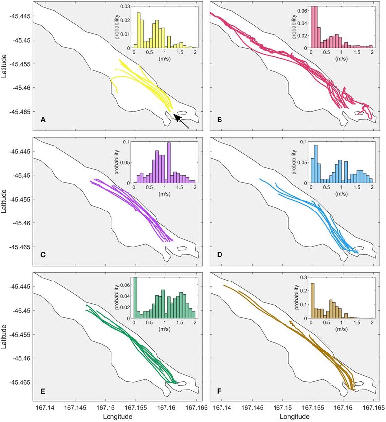
McPherson et al.                                                                                                    Spreading of a Near-Field Plume

nutrient and contaminant loading (Roberts, 1999; Hunt et al.,             (Chen et al., 2009). However, few studies have focused explicitly
2010). Accurate predictions of the ultimate fate and impact of the        on identifying the mechanisms governing lateral spreading.
riverine waters and related material require an understanding of             The physical mechanisms responsible for plume spreading
the plume dynamics over a broad range of spatial scales, typically        can be examined by quantifying horizontal dispersion. While
considered in terms of near and far-field processes.                      advection governs the rate of travel and the direction in which the
    The near-field region, immediately seawards of the plume              plume evolves from a source, dispersion determines the lateral
discharge point, is where the momentum-dominated initial                  and vertical structure of the plume (Stacey et al., 2000; Jones
river discharge transitions into a buoyancy-forced plume. The             et al., 2008). When the vertical dimension is constrained by a
dynamics in this near-field region are governed by turbulent              boundary or stratified layer, such as in the coastal ocean, vertically
mixing, driven by the initial momentum anomaly which                      well-mixed conditions are quickly reached and the dispersion of
enhances velocity shear, and lateral spreading (Hetland, 2005,            scalars tends to occur primarily in the lateral direction (Okubo,
2010). The mid-field region occurs after the inflow momentum              1971).
is depleted by these near-field processes, before transitioning              The mechanisms responsible for horizontal dispersion can be
into the far-field plume that can extend hundreds of kilometers           combined into a single empirical law which relates the rate of
from the river mouth. The far-field plume region is influenced            diffusion [the dispersion coefficient, Kh (m2 s−1 )] of a tracer
by buoyancy, wind stress and rotation (Hetland, 2005). An                 plume to its size (l), i.e., the dispersion is scale-dependent
understanding of the near-field processes, which compete to               (Richardson, 1926; Okubo, 1971). Therefore, the dispersion
determine the plume structure and ultimate redistribution of              coefficient can be expressed generally as,
energy and momentum in the plume (Hetland, 2005; MacDonald
et al., 2007; MacDonald and Chen, 2012; McPherson et al., 2020),                                       Kh = αln                                  (1)
is necessary to properly characterise the local plume behaviour
and understand the implications for the larger coastal ocean.             where the parameters α and n are empirical, and the value of n
    Turbulent mixing and lateral spreading in the near-field              defines the scale-dependence of the dispersion. These empirical
plume region are closely linked (MacDonald et al., 2007; Hetland,         constants incorporate the effects of meteorological (e.g., wind
2010). Vertical mixing of low-momentum, high density ambient              speed, direction) and oceanographic (e.g., stratification, ambient
water into the buoyant plume decelerates the plume, reduces               currents and turbulence) influences, as well as measurement
shear and decreases the density anomaly which in turn slows               errors. The coefficient α is related to the turbulence dissipation
the rate of spreading (McCabe et al., 2009; Kilcher et al., 2012;         rate (ǫ), as the energy transfer between scales is constant (Okubo,
MacDonald and Chen, 2012). Lateral spreading, on the other                1968; Stacey et al., 2000). By applying these parameters to
hand, accelerates the plume due to a shoaling of the surface              models of dispersion, each which represent different dispersion
layer and enhances stratified-shear turbulence (Hetland, 2005;            mechanisms, the drivers of Kh can be determined (Stacey et al.,
MacDonald and Chen, 2012). The role of turbulent mixing in the            2000; Spydell et al., 2007). Note that the nomenclature adopted in
near-field region of the plume system studied in this paper was           this study defines dispersion as the combined processes by which
quantified by McPherson et al. (2020) using direct measurements           turbulence causes irreversible mixing.
and a control volume method. A momentum budget determined                    Measurements of dispersion in the open ocean have found
that the deceleration of the plume was controlled by turbulence           that Kh ∝ l4/3 in a field of homogenous turbulence (Stommel,
stress, with enhanced turbulent kinetic energy (TKE) dissipation          1949; Batchelor, 1950). Studies of dispersion in the surface waters
rates (ǫ) at the base of the plume (maximum ǫ > 10−3 W kg−1 )             of lakes and oceans (Stommel, 1949; Okubo, 1971; LaCasce
(McPherson et al., 2019). Quantifying the role of lateral spreading       and Bower, 2000; Stevens et al., 2004) and in shelf seas (Jones
in the presence of enhanced rates of turbulent mixing is therefore        et al., 2008; Moniz et al., 2014) have corroborated this n =
necessary to characterise the dynamics which govern near-field            4/3 power law. Furthermore, Stacey et al. (2000) and Fong
plume structure.                                                          and Stacey (2003) found that the initial growth of a near-bed
    Spreading dynamics have been examined primarily using                 coastal plume also obeyed the 4/3 law, indicating that open
numerical simulations, which have proved useful for estimating            ocean dispersion theory can be applicable in the near-shore
plume spreading rates and determining plume structure (Hetland            coastal environment. However, the stratification in near-field
and MacDonald, 2008; McCabe et al., 2009; Hetland, 2010;                  river plume systems, where a freshwater surface layer overlies a
MacDonald and Chen, 2012). These model results generally                  coastal ambient layer, is generally stronger than in the open ocean
compare well with direct measurements of plume spreading                  and lakes (Fischer et al., 1979; Nash et al., 2009; Osadchiev, 2018).
obtained using hydrographic surveys and Lagrangian GPS                    This stratification constrains the vertical component of velocity
surface drifters (McCabe et al., 2008; Chen et al., 2009; Kakoulaki       fluctuations which alters the form of dispersion (Fischer et al.,
et al., 2020). However, while the observational methods                   1979; Jones et al., 2008; McPherson et al., 2019). Therefore, it is
demonstrate similar trends, the drifters are also susceptible to          important to understand the driving mechanisms for dispersion
slippage and other near-field processes such as shear or rotation,        in a stratified near-field river plume setting, and compare them to
which influence the perceived lateral spreading rates. A control          those postulated by the 4/3 power law.
volume approach using observations (MacDonald et al., 2007)                  The objective of this study is to quantify the lateral plume
has also been validated for estimating spreading rates, and tends         spreading rate in the near-field region of a buoyant river plume.
to compare better to model results than drifter deployments               The sheltered fjord setting reduces the background energy input

Frontiers in Marine Science | www.frontiersin.org                     2                                         July 2021 | Volume 8 | Article 680874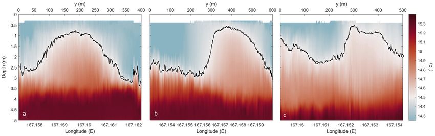
McPherson et al.                                                                                                               Spreading of a Near-Field Plume

from wind and tides, providing an idealised system in which
to examine near-field plume dynamics. Fjord–river interactions
can been directly applied to coastal plumes as the two systems
share many common features, whereby a freshwater inflow
interacts with a coastal ambient (Garvine, 1987; O’Callaghan
and Stevens, 2015). The evolution of the plume width and
lateral spreading rate in the near-field are obtained directly
from GPS surface drifters and lateral hydrographic data, and
then compared with the control volume derived estimates from
McPherson et al. (2020). The role that the fjord setting, with its
steep sidewalls, plays in influencing the lateral spreading of the
plume is also examined. Moreover, the forces that drive lateral
spreading in the near-field are determined using horizontal
dispersion coefficients, obtained from direct observations and
numerical analysis.

2. FIELD SETTING
Doubtful Sound is a glacial fjord located in the far south-
west of New Zealand (45.3◦ S, 167◦ E, Figure 1). The fjord
is approximately 35 km long, typically 7 m (Bowman et al., 1999), and results in
highly stratified conditions. The freshwater input can produce
similar vertical density gradients to those observed in major              coordinate increasing with distance from the discharge point
rivers such as the Columbia and Mzymta Rivers (Kilcher et al.,             (x = 0) toward the end of Deep Cove, and y is the across-channel
2012; Osadchiev, 2018). The depth of the freshwater surface layer          coordinate. This reference frame maintains consistency between
is typically between 2 and 3 m thick (Gibbs, 2001).                        the calculation of lateral plume spreading rates using the different
                                                                           methods outlined below.
3. METHODS AND ANALYSIS
                                                                           3.1. Vessel-Based Survey
The present observations were made during a 2-week long field              A sequence of vessel-based observations within Deep Cove
campaign in March 2016. Over this period, tailrace discharge               were repeated over the course of the field campaign. Along-
rates into Deep Cove were high and relatively steady (Q ≈ 530              channel transects were aligned with the main river discharge,
m3 s−2 ) and the tidal range varied from 0.5 to 1.2 m (Figure 2).          lateral transects cut through the plume perpendicular to its
A range of instrumentation and observational techniques were               trajectory, and oblique (‘zig-zag’) transects captured both lateral
applied to obtain a spatial distribution of the density and velocity       and longitudinal plume evolution (Figure 1C). At least six
fields within Deep Cove. The coordinate system used here is                consecutive lateral transects were repeated during each sampling
based in a channel reference frame, where x is the along-channel           period (Figure 2). Horizontal velocity estimates were obtained

Frontiers in Marine Science | www.frontiersin.org                      3                                                  July 2021 | Volume 8 | Article 680874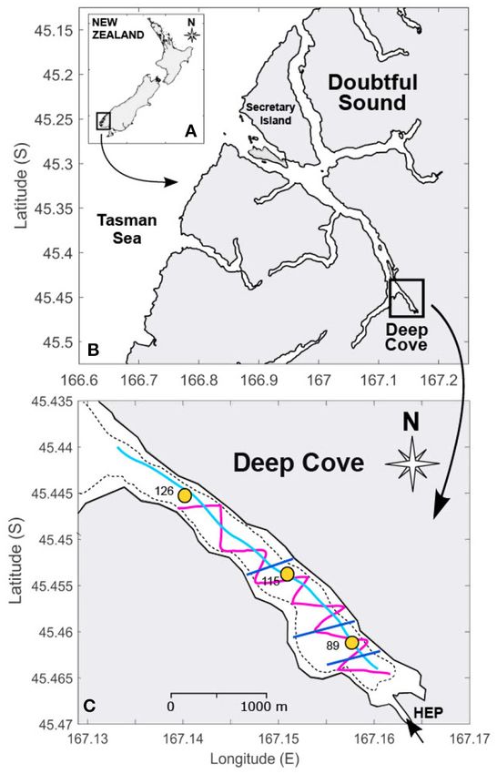
McPherson et al.                                                                                                                  Spreading of a Near-Field Plume

                                                                                          plume depth. The base of the plume is defined as the depth of
                                                                                          maximum stratification. The depth of the plume is then defined
                                                                                          as the distance from the base of the plume to the maximum height
                                                                                          of the bounding isotherm.

                                                                                          3.2. GPS Drifters
                                                                                          Lagrangian measurements of near-surface currents were
                                                                                          made during six GPS drifter experiments. The plume
                                                                                          discharge rate and wind speeds for each experiment are
 FIGURE 2 | Hourly tailrace discharge rate (solid line) and tide (dashed) for the         detailed in Table 1, and wind direction was consistently
 duration of the field experiment. Peak spring tide occurred on 11 March. The
 blue shaded boxes indicate the timing of the GPS drifter experiments and the
                                                                                          up-fjord due to the surrounding steep topography. The
 red were the across-channel vessel transects.                                            headwaters of the fjord absorb the momentum of tidal
                                                                                          oscillations (O’Callaghan and Stevens, 2015) and tides do
                                                                                          not influence near-field mixing here (McPherson et al.,
                                                                                          2019), thus the tidal impact on drifter trajectories is
from a vessel-mounted ADCP (RDI Workhorse, 600 kHz) which                                 not considered.
sampled water velocities in 1 m vertical bins from 2.5 to 41.4                                The drifters each had a cylindrical drogue of height 0.5 m and
m. Near-surface velocities were obtained by applying a linear                             diameter 0.2 m, and were ballasted to measure the upper 0.5 m
fit to the velocity data to extrapolate from 2.5 m to the surface.                        of the water column by a small spherical float. Wind slippage
The extrapolated velocity profiles had compared well to in-                               was minimal as the float had little exposure to wind above the
situ near-surface velocity measurements from previous field                               surface water level. Each drifter was equipped with a GPS receiver
campaigns (McPherson et al., 2019), and were in good agreement                            (Columbia V-900 GPS data logger) which recorded every 1 s. The
with surface plume velocities estimated by the Lagrangian                                 GPS devices have a position accuracy up to 1.5 m, depending
GPS drifters. Currents were rotated according to the local                                on satellite coverage. The drifters were released approximately
bathymetry to determine along-channel (u) and across-channel                              10 m apart across the width of the tailrace discharge point and
(v) velocities. A weighted 10 m ‘bowchain’ was attached to the                            were recovered after ∼ 1 h. A total of 8 drifters were deployed
vessel which comprised temperature (RBRsolo) and CTD loggers                              in the first two experiments then, due to the loss of a GPS
(RBRconcerto) sampling at 2 and 5 Hz, respectively. High-                                 receiver, 7 drifters were deployed and retrieved in the subsequent
resolution profiles of practical salinity and temperature were                            four experiments.
obtained from continuously profiling ’tow-yoed’ CTD loggers                                   The drifters were used to quantify the plume lateral spreading
(RBRconcerto). These data enabled estimation of the buoyancy                              rate by estimating the change in plume width with distance from
frequency from the measured density profiles,                                             the discharge point, following a similar approach applied by Chen
                                      s                                                   et al. (2009). The normalized plume width is given by W/W0 ,
                                              g ∂ρ                                        where W is the plume width at a given location and W0 is the
                                 N=       −                                     (2)
                                              ρ ∂z                                        width of the plume at a reference location. For drifter data, W is
                                                                                          evaluated as the standard deviation of the distances between all
where ρ is the potential density.                                                         drifters in the cross-plume direction at the given location. The
   The lateral transects of temperature from the bowchain were                            plume width is then normalized by W0 . For each GPS drifter
used to quantify vertical (Kz ) and lateral (Ky ) diffusion by                            deployment, W0 is taken as the first estimate of plume width
estimating the change in thickness and width of the plume                                 (W) closest to the tailrace discharge point. This choice of W0
over distance, respectively. While salinity is generally used                             enables W/W0 for each drifter deployment to be compared,
to identify and track freshwater plumes in coastal systems                                despite the variability in the deployment locations of the drifters
(Hetland, 2005), the persistent low-salinity surface layer observed                       in each experiment. For the lateral transects, W0 = 100 m, which
throughout Deep Cove and the wider fjord region, resulting from                           is the measured distance of the width of the tailrace discharge
the tailrace inflow and high rainfall (Gibbs, 2001), makes the                            point (McPherson et al., 2020). Here, W is calculated along each
distinction between the buoyant plume and freshwater surface                              drifter track at intervals of 10 m from the reference point. The
layer less pronounced in the salinity field than in temperature                           uncertainty limits are the minimum and maximum standard
(Figures 3C–E). Thus, temperature was used to define the                                  deviations of all the subsets of the deployed drifters at each 10
plume boundaries in this study (Figures 3A,B). The diffusion                              m interval. The drifter method of estimating plume spreading
components were therefore estimated by,                                                   is independent of drifter speed as plume width is evaluated as
                                                                                          the distance between drifter tracks at a specified point from the
                          1yp2                              1zp2                          reference point, and not at a given time.
                   Ky =               and            Kz =          ,            (3)           Lateral dispersion is then quantified from the continuous
                           tt                                tt
                                                                                          convergence and divergence of drifters from the center of the
where tt is the time taken for the plume to flow between each                             plume. The standard deviation of the distance between the
transect, yp is the width of the plume at its base and zp is the                          drifters and the plume centerline (σr ), defined as the average

Frontiers in Marine Science | www.frontiersin.org                                     4                                       July 2021 | Volume 8 | Article 680874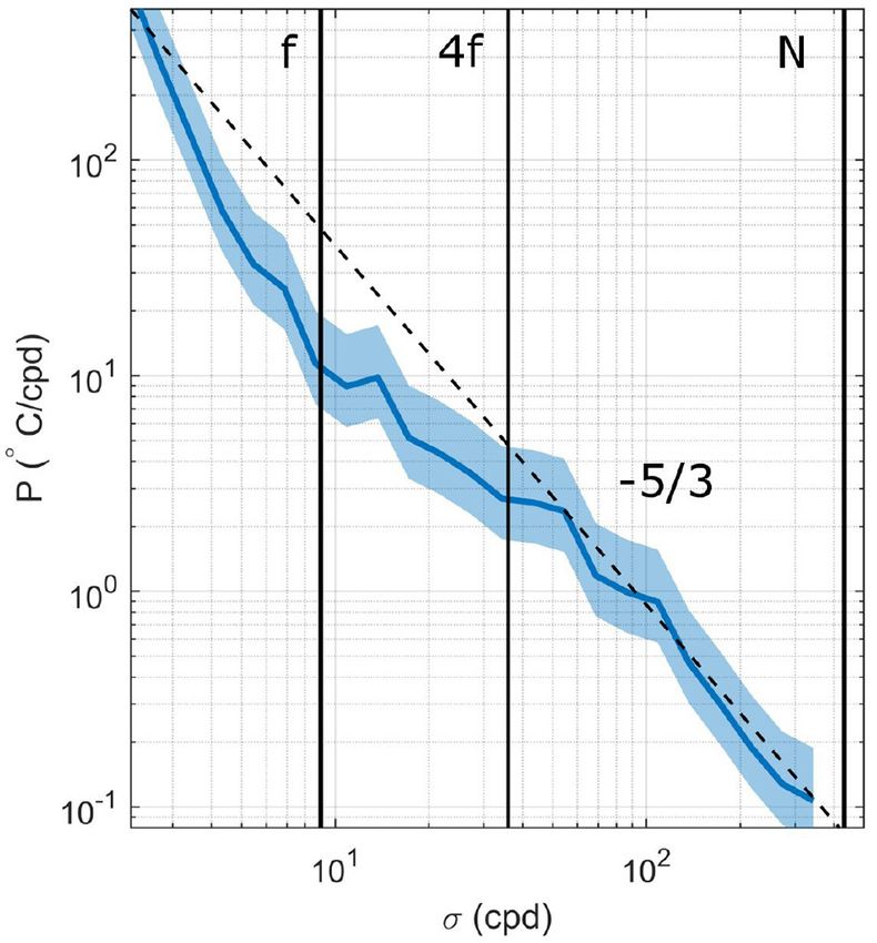
McPherson et al.                                                                                                                          Spreading of a Near-Field Plume

 FIGURE 3 | (A) Vertical and spatial distribution of temperature within Deep Cove, and (B) the expanded temperature timeseries of (A) with respect to distance from
 the discharge point. The horizonal lines in (B) separate each transect. Mean profiles of (C) temperature, (D) salinity, (E) density (σt ), (F) buoyancy frequency-squared
 (N2 ), and (G) along-channel velocity (u) from inside (solid) and outside (dashed) the plume. The path of the transect relative to the fjord in (A) can be seen in
 Figure 1C. The 14, 14.5 and 15◦ C isotherms are shown in (A), and the 14.5◦ C isotherm in (B). The dotted line in (G) shows the depth above which the velocity was
 interpolated. The arrows in (A) and (B) indicate the direction of tailrace inflow (Q), from right to left.

drifter track, was used to calculate the diffusion coefficient,                          Further details about this field campaign can be found in
                                              2 (t
                                                                                         McPherson et al. (2019). Velocity measurements were obtained
                                         dσr d )                                         from an upwards-facing Acoustic Doppler Current Profiler at
                              Kh (l) =                                         (4)
                                           2dt                                           10 m (ADCP; RDI Workhorse, 600 kHz), set to record an
where td is the diffusion time (i.e., the time elapsed since the                         ensemble every 3 min in 2 m vertical bins. Spectral analysis was
individual drifter deployment) and l = 3σr is the scale of                               conducted on the velocity observations (Emery and Thomson,
diffusion (Okubo, 1971). Horizontal  plume spreading is generally                        2001) in which the time series was split into half-overlapping
                         q                                                               intervals equivalent to the inertial frequency, and the spectrum
anisotropic thus σr =              (σx2 + σy2 ), where σx , σy denote the
                                                                                         was computed using Welch’s periodogram method.
standard deviations in the along and across-channel directions,
respectively (Stocker and Imberger, 2003).
                                                                                         3.4. Control Volume Methods
3.3. Moored Timeseries Data                                                              Plume lateral spreading rates can also be quantified using
Contributions to results in section 5.3.1 were from three near-                          the control volume method, where measured quantities are
surface moorings deployed in September 2015 (Figure 1C).                                 connected to plume dynamics over a defined finite region of

Frontiers in Marine Science | www.frontiersin.org                                    5                                               July 2021 | Volume 8 | Article 680874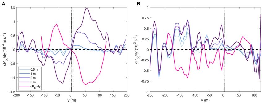
McPherson et al.                                                                                                        Spreading of a Near-Field Plume

TABLE 1 | Summary of drifter deployments and conditions.                         over 1.5 ms−1 , which overlay a relatively stationary ambient
                                                                                 below 5 m (Figure 3G). The ambient surface layer currents were
Day                      Wind speed                 Discharge     Total
                                                                                 weak (< 0.1 ms−1 ), thus the outer plume boundary can also
(March 2016)                (ms−1 )                 (m3 s−1 )   retrieved
                                                                                 be defined by speeds of 0.2 ms−1 . The near-surface velocity
04                          5.6–6.8                   515          8             field shows the plume decelerates as it propagates downstream.
06                          0.8–2.4                   527          8             Maximum surface velocities at the plume centerline decreased
07                          1.5–1.8                   501          7
                                                                                 from 1.05 ms−1 to 0.2 km downstream of the tailrace discharge
08                          4.8–6.0                   530          7
                                                                                 point to 0.81 and 0.65 ms−1 at 0.5 and 1.5 km downstream,
09                          2.3–2.6                   532          7
                                                                                 respectively, (Figure 4A). Flow speeds tended toward zero with
13                          4.1–5.3                   536          7
                                                                                 lateral distance from the plume centerline, into the surrounding
                                                                                 surface ambient. The near-surface plume measurements
                                                                                 compared well to the velocities derived from the GPS drifters,
                                                                                 estimated as the time derivative of the coordinate position. The
the flow field, termed a control volume. Freshwater conservation                 drifters initially moved at speeds of ∼ 1.7 ms−1 near the tailrace
is applied to estimate plume width (b) in the control volume                     discharge point and decreased to approximately 0.6 ms−1 toward
region (MacDonald and Geyer, 2004; Chen et al., 2009). Details                   the seaward end of Deep Cove (Figure 5). Maximum speeds of
of the control volume over the near-field plume region in Deep                   over 2 ms−1 were recorded near the discharge point.
Cove can be found in McPherson et al. (2020). Horizontal scale-
dependent dispersion is then determined from the growth of b                     4.2. Techniques for Evaluating Lateral
with distance from the tailrace discharge point,                                 Plume Spreading
                                                                                 4.2.1. GPS Drifters
                b(x) = ((2 − n)βb1−n    2−n 1/(2−n)
                                 0 x + b0 )                            (5)       Estimates of plume width derived from the 6 GPS drifter
                                                                                 deployments indicate an evolving plume structure as the plume
where β = 12α/(Ub0 ) represents the magnitude of dispersion                      propagates downstream (Figure 6). The drifter tracks show
using the mean along-channel velocity U, and b0 is the initial                   consistent behaviour over sections of the trajectories, with the
plume width (Fong and Stacey, 2003). A non-linear least squares                  plume width thinning and thickening over the same intervals.
fit of the control volume estimates of b to Equation (5) is                      A general reduction in plume width from W/W0 = 1 between
taken and both β and n are treated as adjustable parameters.                     the tailrace discharge point to 1 km downstream is observed in
By optimising for n and α using this fit, these parameters can                   all transects, reaching a minimum of W/W0 = 0.2, before the
be compared to the empirical estimates from Equation (4). The                    plume begins to spread laterally and W/W0 increases toward
method has been used to estimate horizontal dispersion in both                   1 at 1.5 km. The three deployments that propagated further
near-coastal systems and the open ocean (Stacey et al., 2000; Fong               downstream show an overall decrease in W/W0 toward 2.5 km.
and Stacey, 2003; Jones et al., 2008; Moniz et al., 2014).                       However, little to no lateral plume spreading occurred over the
                                                                                 length of Deep Cove. The estimates of W/W0 at the end of
4. RESULTS                                                                       each transect were generally smaller than 1, with fluctuations of
                                                                                 W/W0 between 0.7and0.9 over the length of each deployment.
4.1. Near-Field Water Column Structure                                           This reflects the observed drifter trajectories where the majority
Observations from the bowchain and tow-yoed CTD showed a                         of drifters remained within 10 m of each other over the duration
highly-stratified upper water column with a 2 m thick freshwater                 of each experiment (Figure 5). The maximum W/W0 = 3.4
(σt ≈ 1 kg m−3 ) surface layer overlaying a sharp density                        occurred during the 04 March experiment when two drifters were
interface, and a dense, oceanic ambient (σt = 24 kg m−3 )                        detrained from the mean flow and diverged from the body of the
below 5 m (Figures 3B–E). The zig-zag temperature transects                      drifter pack at approximately 1 km downstream from the inflow
illustrate the evolving structure and path of the buoyant plume                  (Figure 5A).
within the surface layer (Figure 3A). The 3 m thick plume was
observed in the surface layer as a core of water approximately 1◦                4.2.2. Lateral Vessel Transects
C warmer than the 13.6◦ C ambient surface layer (Figures 3A–C).                  The lateral spreading and evolving structure of the surface plume
The plume boundary can thus be defined by an isotherm of                         can be clearly identified in mean transects of temperature and
14.5◦ C. Maximum plume temperatures were found at the base of                    velocity at increasingly downstream locations. Near the tailrace
the surface layer, toward the core of the plume (∼ 14.9◦ C) where                discharge point, the buoyant plume was a distinct symmetrical
warmer water was entrained from the ambient below (15.5◦ C)                      core of warmer water (> 14.5◦ C) within the 3 m thick ambient
(Figure 3C). The plume was confined to the surface layer by                      surface layer (Figure 7a). The surface layer overlays a sharp
strong salinity-induced stratification (N 2 = 10−1 s−2 ) in the                  thermocline and well-mixed 15.5◦ C ambient water below 4 m.
pycnocline (Figure 3F). Generally weaker values were observed                    The plume width at 0.2 km from the discharge point was 268 m,
within the plume layer (N 2 = 10−2 s−2 ) and reduced toward                      compared to a fjord width of approximately 800 m. At 0.5 km
zero with depth below the interface to 10 m.                                     downstream, the width of the near-symmetric core had increased
    The velocity structure of the near-field region was                          to 312 m (Figure 7b) while, farther downstream at 1.5 km, the
characterised by a fast-flowing surface plume with speeds                        plume had spread almost uniformly across the vessel transect and

Frontiers in Marine Science | www.frontiersin.org                            6                                      July 2021 | Volume 8 | Article 680874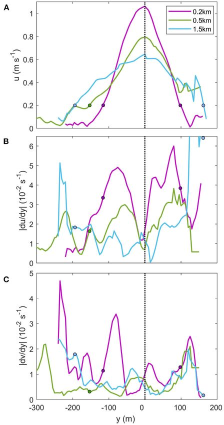
McPherson et al.                                                                                                                 Spreading of a Near-Field Plume

                                                                                        0.2 ms−1 , increased laterally from 225 to 355 m over the 1.3 km
                                                                                        distance. Along and across-channel velocity shear at the base of
                                                                                        the plume were derived using the vessel-mounted ADCP. Strong
                                                                                        velocity shear occurs at either side of the plume centerline at each
                                                                                        downstream transect, with peaks corresponding the location of
                                                                                        the plume edges (0.2 ms−1 , Figure 4A), before tending toward
                                                                                        zero both toward the plume centerline and into the surrounding
                                                                                        ambient. Maximum values of |du/dy| ≈ |dv/dy| ≈ 10−2 s−1
                                                                                        peaked within 0.2 km of the tailrace discharge point, where plume
                                                                                        speeds were greatest (u > 1 ms−1 ) (Figure 4). The peaks of
                                                                                        velocity shear decreased with distance from the discharge point
                                                                                        as the plume decelerated and moved laterally away from the
                                                                                        centreline as the plume spread. Farther downstream at 1.5 km,
                                                                                        the maximum |du/dy| and |dv/dy| decreased by half and peaked
                                                                                        toward the edges of the transect where the plume boundaries
                                                                                        were approached (Figures 4B,C).

                                                                                        4.3. Techniques for Evaluating Dispersion
                                                                                        4.3.1. GPS Drifters
                                                                                        A diffusion diagram provides a means of predicting the rate
                                                                                        of lateral spreading and the scale-dependence of the dispersion
                                                                                        rates. Dispersion rates for the plume derived from the GPS
                                                                                        drifters (using Equation 4) are shown as a function of their
                                                                                        scale. As expected, the lateral component of dispersion (Ky ) was
                                                                                        much larger than the longitudinal dispersion (Kx ) component,
                                                                                        and both Kx and Ky increased with the scale of mixing
                                                                                        (Figure 8). Estimates of Kx = 0.3 − 1.0 m2 s−1 were
                                                                                        observed at diffusion scales of 0 < l < 120 m, while Ky
                                                                                        was at least one order of magnitude greater for larger scales,
                                                                                        ranging from Ky = 1.4 − 14.1 m2 s−1 between 102 <
                                                                                        l < 103 m. Expressing the estimates in the form of Kh =
                                                                                        αln (Equation 1), the line of best fit yielded α = 0.0017
                                                                                        m2/3 s−1 and n = 1.38 ± 0.23. The errorbars show 95%
                                                                                        confidence intervals of the slope over 1,000 bootstrap samples.
                                                                                        Most of the latitudinal and longitudinal diffusion estimates
                                                                                        fall within the 95% confidence intervals on either side of the
 FIGURE 4 | The evolving mean (A) across-stream velocity, and velocity shear            predicted values.
 of (B) along-channel and (C) across-channel velocities at downstream
 locations from the discharge point. Velocities are from 2.5 m below the
 surface. The across-channel distance (y) is relative to the centre of the plume,
 defined as the location of maximum u. The coloured circles represent the
                                                                                        4.3.2. Lateral Vessel Transects
 location of the plume edge, defined by 0.2 ms−1 . (A) The mean velocity                Estimates of plume dispersion rates from the lateral vessel
 transects were averaged over at least six consecutive lateral transects from           transects of temperature (Figure 7) can also be obtained. Using
 the vessel-mounted ADCP on 09 March 2016.                                              the 14.5◦ C isotherm as the plume boundary and applying
                                                                                        Equation (3), the results provided an alternate estimate of Ky =
                                                                                        29.8 m2 s−1 and a vertical diffusion component of Kz =
had a width of 371 m (Figure 7c). The thermocline had become                            1.4 × 10⁻⁴ m2 s−1 for the distance between the 0.2 and 1.5
more diffuse with distance from the inflow and thickened down                           km transects. This Kz is comparable to the vertical diffusivity
to 4.5 m.                                                                               measured in other river plumes (Hetland, 2005; Horner-Devine
    The evolution of the near-surface velocity field also shows the                     et al., 2009) which suggests that Equation (3) provides an
lateral spreading of the plume. At the tailrace discharge point,                        accurate first-order estimate of bulk diffusion. The Ky estimates
the plume has a near-Gaussian appearance which flattens and                             derived from both Figure 7 and other repeated lateral transects
spreads laterally as it propagates downstream (Figure 4A). The                          of temperature agree well with the drifter-derived horizontal
distance between the outer plume boundaries, here defined by                            diffusion results (Figure 8).

Frontiers in Marine Science | www.frontiersin.org                                   7                                        July 2021 | Volume 8 | Article 680874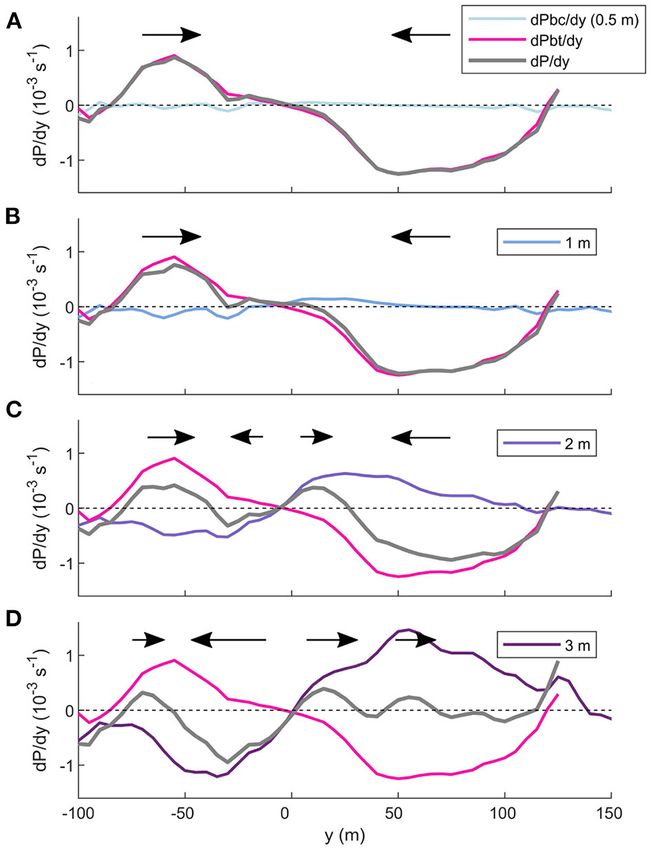
McPherson et al. Spreading of a Near-Field Plume
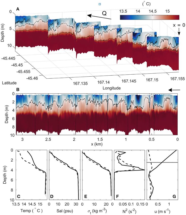
FIGURE 5 | The trajectories of the multiple GPS drifters released near the entrance of the tailrace discharge point, where (A–F) are the six deployments,
corresponding to the days outlined in Table 1, respectively. On the upper right corner of each plot is a histogram of flow velocities of all the drifters in each experiment
(ms−1 ). The histograms are normalised by the maximum of the distribution. The arrow in (A) indicates the tailrace discharge point and the direction of flow.
5. DISCUSSION method. This control volume technique used hydrographic
observations from along and across-fjord transects, and is
5.1. Comparison of Spreading Rates detailed in McPherson et al. (2020).
Between Techniques Estimates of plume width derived from the across-channel
The rate of plume lateral spreading was quantified using two hydrographic transects generally compared well to the estimates
different observational methods; Lagrangian GPS drifters which derived from the control volume method (Figure 9). The control
measured near-surface plume velocities directly (Figure 6) and volume results show that W/W0 increased from 1 close to the
lateral transects of temperature and velocity fields (Figures 4, tailrace discharge point to W/W0 = 1.8 over 3 km downstream,
7). These directly observed results can then be compared to indicating that the plume spread laterally in the near-field region
estimates of plume width determined by a control volume as it propagated seaward. The estimates of W/W0 derived
Frontiers in Marine Science | www.frontiersin.org 8 July 2021 | Volume 8 | Article 680874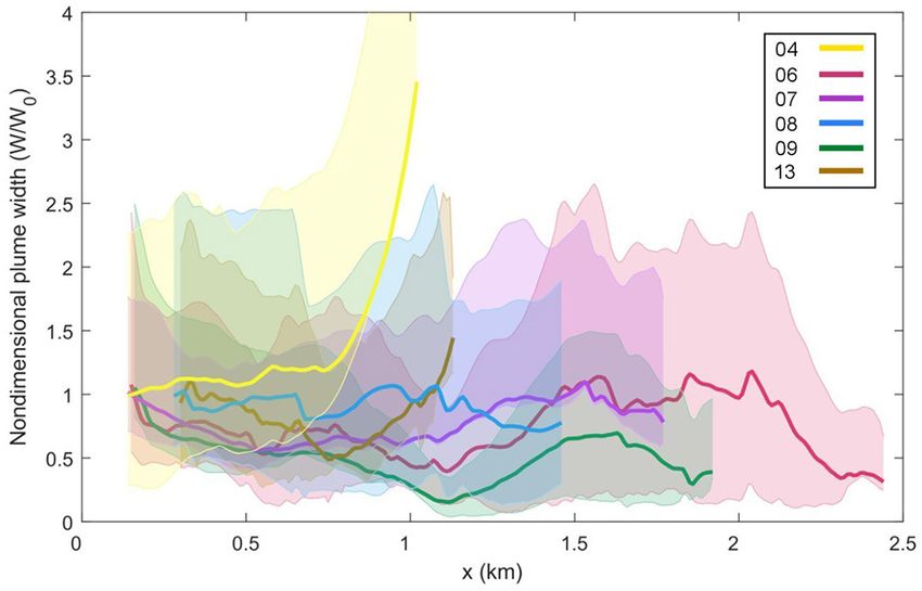
McPherson et al.                                                                                                                         Spreading of a Near-Field Plume

from the repeated lateral transects of temperature and velocity,                      pattern of db/dx in the initial 1.5 km, with weaker horizontal
using 14.5 ◦ C and 0.2 ms−1 as the definitions of the plume                           spreading rates in the first 0.5 km and an increase toward 1.5
boundary, respectively, correspond well at the three downstream                       km. Further downstream, there is a slowing of plume spreading
locations. They all show a consistent increase in W/W0 over                           toward the end of Deep Cove. The highest lateral spreading
the along-channel distance and are in good agreement with the                         rates are generally derived from between the lateral transects of
control volume plume width estimates. The estimates of W/W0                           temperature and velocity, with db/dx ≈ 0.05 between 0.2 and
derived from the average GPS drifter trajectory (Figure 6) are
generally smaller than the other observed values, suggesting an
underestimation of plume width using this method.
    While a general increase in W/W0 over the length of Deep
Cove was observed in both the control volume and transect data,
the variability in the measurements highlights an evolving along-
channel lateral spreading rate (db/dx). Over the total 3 km near-
field region, db/dx = 0.045 from the control volume estimates.
However, this rate increases and decreases over different sections
of Deep Cove. All methods show an agreement in the evolving

                                                                                       FIGURE 8 | Okubo-style diffusion diagram of mean lateral (Ky , circles),
                                                                                       longitudinal (Kx , stars) and total diffusion (Kh , triangles) against the scale of
                                                                                       diffusion (l). All diffusion component estimates were derived from the 6 GPS
                                                                                       drifter trajectories (Figure 5) and Ky from two sets of mean lateral temperature
 FIGURE 6 | The non-dimensional plume width (W/W0 ) for each GPS drifter               transects at the three downstream locations (green) (Figure 1C). Error bars
 experiment with respect to along-channel distance from the discharge point            denote a 95% bootstrap confidence interval of the slope (dashed lines). The
 (x). The shaded regions indicate the uncertainty for each deployment. The             two vertical lines (dotted) represent the average width of the plume (lp ) and the
 drifter trajectories were averaged over 10 m.                                         fjord (lf ).

 FIGURE 7 | Mean vertical distribution of temperature of across-channel transects in the near-field plume region taken (a) 0.2 km, (b) 0.5 km and (c) 1.5 km
 downstream of tailrace discharge point. The plume boundary was defined by the isotherm 14.5◦ C (black lines), and the plume edge is indicated by the white circles on
 the isotherm. These edges were determined from the gradient of the depth of the isotherm. Temperature was recorded by the bowchain and averaged over at least
 six consecutive lateral transects.

Frontiers in Marine Science | www.frontiersin.org                                 9                                                 July 2021 | Volume 8 | Article 680874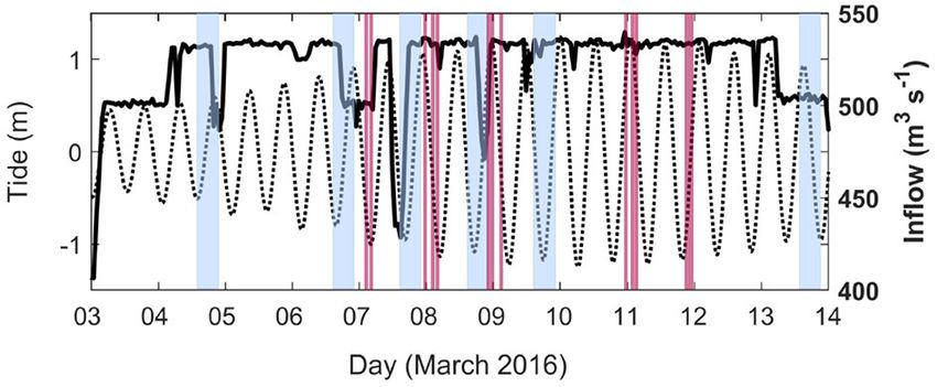
McPherson et al.                                                                                                                        Spreading of a Near-Field Plume

0.5 km increasing to between 0.04 and 0.09 between 0.5 and 1.5                          or in fact quantified a different process that was locked to the
km. Estimates of db/dx from the control volume method are at                            near-surface.
the lower range over the same intervals, peaking at 0.05 at 1.5                             This change in db/dx in space is not surprising as the
km. While the corresponding horizontal spreading rate from the                          spreading rate is determined by the initial momentum from
GPS drifters also shows this evolution of db/dx, with an initial                        the variable plume inflow (Figure 2), the density difference
weaker db/dx and an increased rate between 0.5 and 1.5 km, the                          between the freshwater surface layer and ambient water below,
estimates of db/dx remain one order of magnitude smaller than                           and the degree of vertical mixing at the interface (Chen et al.,
the control volume estimates over the length of the track. The                          2009). Thus the effect of the enhanced shear-driven mixing
good agreement between the estimates of plume width and db/dx                           observed at the base of the plume (McPherson et al., 2019)
from the control volume and lateral vessel transects (Figure 9)                         which weakens the density gradient at the interface as the plume
indicates that either the drifters underestimated the plume width,                      propagates downstream (Figure 7) would in turn reduce the
                                                                                        lateral spreading rate.
                                                                                            The discrepancy between the results can be examined by
                                                                                        considering what the GPS drifters actually measured in this field
                                                                                        setting. While estimates of lateral spreading from drifters in other
                                                                                        river plume systems have generally compared well to results
                                                                                        from numerical and other observational techniques (Hetland and
                                                                                        MacDonald, 2008; Chen et al., 2009; McCabe et al., 2009), drifters
                                                                                        are also susceptible to meteorological and other oceanographic
                                                                                        factors. A drifter consisting solely of a surface float with no
                                                                                        drogue provides velocities and a trajectory that are a combination
                                                                                        of surface advection, Stokes drift (an extra wave-induced force
                                                                                        at the water surface) and direct wind forcing (Lumpkin et al.,
                                                                                        2017). However, the impact of these external forcings on the GPS
                                                                                        drifters used in the experiments conducted in Deep Cove were
                                                                                        minimized by their design. The effects of wind on the trajectories
 FIGURE 9 | The evolution in non-dimensional plume width (W/W0 ) with                   of the drifters in Deep Cove was reduced by having very little
 distance from the discharge point estimated by three observational methods:            of the drifter visible above the water, by conducting the GPS
 lateral transects of temperature (triangles) and velocity (circles), a control         drifter experiments when wind speeds were low (Table 1), and
 volume method (red) (McPherson et al., 2020) and the average W/W0
                                                                                        by including a ballast centered at 0.5 m beneath the surface.
 calculated from the six GPS drifter deployments (Figure 6) (blue). The estimate
 of W for each method was normalized by W0 , where W0 = 100 m for the                   The ballast also ensured the drifter was largely unaffected by the
 transects and control volume, and W0 = W(1) for the drifter deployments. The           motion due to drift beneath the surface-wave-driven Stokes layer.
 average plume width from the drifters was estimated with a minimum of three                In Deep Cove, the drifters tended to remain clustered together
 measurements for a standard deviation (shaded blue area).                              within the body of the plume with no evidence of horizontal

 FIGURE 10 | Horizontal baroclinic pressure gradient from within the plume layer at 0.5, 1, 2, and 3 m below the water surface, and barotropic pressure gradient (pink)
 at (A) 0.25 km and (B) at 1.5 km downstream of the tailrace discharge point (Figure 1C). The vertical dashed lines illustrates the centre of the plume.

Frontiers in Marine Science | www.frontiersin.org                                  10                                              July 2021 | Volume 8 | Article 680874
McPherson et al. Spreading of a Near-Field Plume
spreading (Figure 5). Over the initial 1 km, all drifter trajectories
tended to show a decrease in plume width, before increasing
further again downstream (Figure 6). The high flow speeds
measured by the drifters (Figure 5) indicate the drifters remained
within the main flow. The clustering of the drifters near the
plume centerline is likely caused by a convergence of surface flow
that concentrated the drifters in regions of high velocity within
the center of the plume (Hetland and MacDonald, 2008).
The density and pressure gradients in the surface layer suggest
this convergence of surface water occurred in the initial 1 km.
Density and pressure in the surface layer are greatest within the
center of the plume (Figure 3E) due to the enhanced entrainment
of high density ambient water into the low density surface plume,
driven by strong vertical mixing (McPherson et al., 2019). This
vertical mixing creates a horizontal density gradient at the base
of the plume. The corresponding horizontal baroclinic pressure
gradient component is therefore greatest at 3 m below the
surface, and peaked on either side of the plume centreline at
both 0.25 and 1.5 km downstream of the inflow (Figure 10). The
baroclinic pressure gradients tends toward zero at the surface.
The barotropic pressure gradient also displays corresponding
peaks at eiher side of the plume centerline, though the peaks of
either pressure component are of an opposite sign.
By combining the across-channel baroclinic and barotropic
pressure gradients, the total across-channel pressure gradient
determines the direction and magnitude of the near-surface
flow (Figure 11). At the surface, the total pressure gradient
is dominated by the barotropic component, as the baroclinic FIGURE 11 | The balance of pressure gradient components within the surface
pressure gradient is weakest at 0.5 m (Figure 11A). The positive layer at 0.2 km from the tailrace discharge point. The barotropic (pink) and
total pressure gradient to the left of the plume centerline and the baroclinic components sum to equal the total pressure gradient (grey). The
negative to the right indicates a strong flow converging toward baroclinic component is calculated at (A) 0.5 m, (B) 1 m, (C) 2 m, and (D) 3 m
below the surface. The black arrows indicate the direction of the flow across
the center of the plume. With depth, the baroclinic component
the mean transect as a result of the total pressure gradient. The size of the tail
increases and begins to influence the total pressure gradient, of the arrow scales with the strength of the flow.
thus the direction of near-surface flow. A lateral diverging flow
from the centre of the plume is already apparent at 2 m, while
there is still exists a stronger converging flow outside 50 m
(Figure 11C). At 3 m, the baroclinic component dominates the plume. This near-surface divergence of flow from the plume
total pressure gradient (Figure 11D). This results in a strong centerline is also reflected in the GPS drifter trajectories which
lateral flow of plume water away from the centerline, driving show an increase of plume width from 1 to 1.5 km. The rate
the lateral spreading of the plume. The lateral velocity gradient of plume spreading over this distance derived from the GPS
(dv/dy) also illustrates diverging velocities at 2.5 m below the drifters compared relatively well to db/dx from the control
surface, peaking at the edges of the plume (Figure 4C). volume estimates (Figure 9). Toward the end of Deep Cove, the
This balance of flow convergence toward the plume centerline drifters measured a decrease in plume width (Figure 9) which
at the near-surface and divergence from the centerline at the suggests another reversal of the lateral pressure components and
plume base can also be demonstrated in the Gaussian shape a convergence of near-surface flow.
of the near-field plume in the lateral transects of temperature These horizontal density, pressure and velocity gradients
(Figure 7). The wider base illustrates the lateral spreading of (Figures 3B, 4, 10, 11), and the structure of the plume (Figure 7),
the plume driven by the baroclinic pressure gradient, while suggests that the GPS drifters, drogued to the upper 0.5 km, were
the narrowing toward the water surface indicates the near- concentrated within the plume core over the intial 1 km by near-
surface convergence. surface convergence, driven by the barotropic pressure gradient.
Further downstream at 1.5 km, the role of the pressure The clustering of drifters about the plume centerline and within
gradient components are reversed (Figure 10B). The barotropic the main flow (Figure 4) meant that both the plume width and
component drives a near-surface divergence of flow while the lateral spreading rate were not accurately measured, but also that
corresponding baroclinic pressure gradient shows a convergence the drifters were then dominated by the strong along-channel
of flow, the strength of which increases with depth. The advection, which was a dominant component of the plume
barotropic pressure gradient tends to dominate throughout dynamics along the whole 3 km near-field region (McPherson
the surface layer which drives a total lateral spreading of the et al., 2020). This resulted in an underestimation of the overall
Frontiers in Marine Science | www.frontiersin.org 11 July 2021 | Volume 8 | Article 680874McPherson et al. Spreading of a Near-Field Plume
lateral spreading rate by the drifters in comparison to the divergence drove the deceleration. This translates to a greater
other observational methods (Figure 9). Further downstream, lateral spreading rate in the Columbia River, db/dx = 0.16
the barotropic pressure gradient acted to diverge the near- (Kilcher et al., 2012), which was one order of magnitude larger
surface flow away from the centerline which produced a than in Deep Cove. In Deep Cove however, where turbulence
comparable lateral spreading rate to the other observational stress was high, the spreading term was negligible and the
methods employed, before converging again toward the end of internal stress similarly controlled the plume deceleration. The
Deep Cove. balance of dynamics in each near-field setting suggests that the
increase in internal stress reduces the spreading rate. When the
internal stress increases relative to the other near-field processes,
5.2. Comparison With Other River Plume the enhanced turbulence at the interface drives a reduction in
Systems the density difference between the ambient and surface and
While the drifters converged toward the plume centerline at therefore a reduced lateral spreading rate. Thus, the high ǫ
the near-surface and tended to underestimate the plume width, in Deep Cove could be responsible for the slower horizontal
the results from the hydrographic transects and control volume spreading than typically observed for near-field plumes with
also suggest a slower lateral spreading rate than typically found weaker turbulent mixing.
in near-field settings. The coastal river plumes conventionally While the enhanced turbulent mixing at the base of the plume
studied generally show radial expansion and splaying streamlines in the near-field is likely to reduce the rate of lateral plume
(Hetland and MacDonald, 2008; McCabe et al., 2009; Kakoulaki spreading, the surrounding topography and its impact on plume
et al., 2020), and adhere to aphorizontal spreading rate for a evolution is also relevant in this system. The trajectories of the
two-layer gravity current of (g ′ H)/2 (Farmer et al., 2002). GPS drifters highlight the proximity of the fjord sidewalls to
In the near-field region of Deep Cove, where g ′ is calculated the mean plume flow (Figure 5). While the role of the sidewalls
using an across-channel 1σt from Figure 3E, this equates to a on the lateral plume spreading rate cannot be quantified, they
bulk horizontal spreading rate of ∼ 0.19 ms−1 . With a mean are able to explain the circulation pattern in the surface layer
along-channel plume velocity of 0.8 ms−1 , the plume would by driving the barotropic pressure gradient and convergence
theoretically spread by ∼ 450 m over the 3 km near-field region of near-surface flow. The plume spreads laterally, from high to
(db/dx = 0.15). However, the observational results did not agree low pressure, as it propagates downstream (Figure 10). However,
with these estimates. The plume width increased from 105 to the sidewalls act as a physical barrier which prevents the
240 m over the length of Deep Cove, with a total spreading rate continued and uninhibited lateral spreading of the plume. As the
that was slower than theoretical rate by one order of magnitude strong vertical density gradients (Figures 3E,F) also prohibit the
(db/dx = 0.045 m−1 , Figure 9). downwelling of the surface ambient water, the surface water is
The difference between these lateral spreading rates could be then pushed up against the fjord sidewalls and increases the water
attributed in part to the intense vertical mixing at the base of the height there. This creates a barotropic pressure gradient across
plume in Deep Cove. Enhanced turbulent mixing has been shown the width of Deep Cove which drives the water back toward the
to drive interfacial stress which is a dominant force acting to center of the fjord and the plume. However, as the baroclinic
decelerate the near-field plume (Chen et al., 2009; McCabe et al., pressure gradient is zero at the surface but greater than the
2009; McPherson et al., 2020). The deceleration is controlled barotropic component at 3 m (Figure 11), the water converges
by entraining low-momentum ambient water into the surface at the surface but is forced to diverge laterally at the base of
layer, simultaneously mixing high-density ambient water into the plume.
the freshwater surface layer, thus reducing the density gradient However, a uniform convergence of near-surface flow along
and slowing lateral spreading (Hetland, 2010). In comparison to the fjord was not observed. The lateral pressure gradient
typical estimates of ǫ in coastal environments, the measurements components showed a transition from near-surface convergence
observed in the near-field region of Deep Cove are orders of in the initial 0.25 km to divergence further downstream at
magnitude greater. The highly stratified interface (N 2 = 10−1 1.5 km (Figure 10) which was reflected in the trajectories of
s−2 , Figure 3F) supports the intense shear generated by the the GPS drifters as they propagated downstream (Figure 6).
high flow speeds (u > 1.5 ms−1 , Figure 3G), resulting in This along-channel change in near-surface flow could also
surface-intensified turbulence (ǫ > 10−3 W kg−1 ) (McPherson be attributed to the sidewalls driving a form of oscillatory
et al., 2019). This corresponds to enhanced surface-intensified motion, such as a seiche, which propagates throughout the
turbulence stress, over one order of magnitude greater than the fjord basin. The initial expansion of the plume as it enters
peak stress in the Columbia River (Kilcher et al., 2012). the fjord, no longer confined by the tailrace channel, forces
Comparing the balance of terms in a near-field momentum the surrounding ambient water toward the fjord sidewalls. The
budget between Deep Cove and the Columbia River shows that barotropic pressure gradient is formed as described above and
the enhanced vertical mixing in Deep Cove is likely linked drives the near-surface convergence. However, this returning
to the reduced corresponding lateral spreading rate. In the flow toward the center of plume could also be an oscillation
Columbia River, where internal stress was weaker, the role of which continues to propagate downstream and move laterally,
lateral spreading in balancing the total momentum budget was impacting the barotropic pressure gradient and thus the drivers
much greater than in Deep Cove. The spreading term balanced of plume spreading, reflected in the trajectories of the GPS
the acceleration terms in the surface layer, and the internal stress drifters. However, the current spatial and temporal resolution
Frontiers in Marine Science | www.frontiersin.org 12 July 2021 | Volume 8 | Article 680874McPherson et al. Spreading of a Near-Field Plume
of the data is unable to fully resolve any basin-wide oscillatory
motion and its impact on the plume. The change in the fjord
topography also impacts the plume spreading. The fjord is wider
between 0.25 and 1 km as a bay exists to the south of the inflow
(Figure 1C), before narrowing further downstream. As described
above, the sidewalls restrict lateral spreading of both the plume
and the surface ambient, thus any narrowing or widening of the
sidewalls relative to the location of the plume would also affect
the lateral pressure gradients and spreading.
There have been no observational field studies of the spreading
dynamics of topographically-constrained plumes; river plumes
typically studied generally exhibit a discharge perpendicular to
the coast with no lateral boundaries (Yankovsky, 2000; Hetland
and MacDonald, 2008; Chen et al., 2009; Kakoulaki et al., 2020).
However, a change in drifter patterns was observed when GPS FIGURE 12 | Plume width (b) as a function of distance from the tailrace
and modelled drifters, deployed near the mouth of a weakly- discharge point. The best-fit line with scale-dependency n = 1.39 ± 0.35
stratified tidal inlet, left the constrained tidal channel and (solid) was determined using the length-scale model of Equation (5). Dashed
reached the mouth of the inlet (Spydell et al., 2015). Within lines are the 95% confidence limits of the line of best fit.
the channel, the drifters were generally retained in the main
flow while, upon exiting the inlet, the lateral spreading rates
increased. While a decrease in flow velocities with downstream
distance was observed, which could balance the increase in combines estimates of diffusion from the GPS drifters and
horizontal spreading, the impact of the channel walls on the hydrographic transects (Figure 8). Based on scale, the estimates
drifter trajectories and spreading rate were not considered. It is of lateral diffusion observed here are comparable to other plume
not unlikely that the same barotropic pressure gradient, from inflows (Yankovsky, 2000; Hunt et al., 2010). The line of best-fit
the increased sea surface height at the sidewalls of the channel, applied to these estimates yielded n = 1.38 ± 0.23. This observed
produced a convergence of flow which contributed to the drifters n is not inconsistent with, and indeed compares relatively well
clustering together in the main flow. Though the fjord sidewalls to, the theoretical n = 4/3 which suggests scale-dependent
appear to influence the near-surface circulation in Deep Cove, behaviour following the 4/3 law.
the relative roles of the enhanced turbulence and topography on Furthermore, the plume width model (Equation 5), using
the reduced lateral spreading rate relative to other plume systems estimates of b derived from the control volume, can also be
remains unclear. used to quantify the plume’s scale-dependent lateral dispersion.
A non-linear least-squares fit of b is applied to Equation (5),
5.3. Lateral Dispersion setting b0 = 128 m and U = 1.1 ms−1 , and optimising for n
While advection governs the evolution and transport of the and β, gives a best-fit of n = 1.39 ± 0.35 and β = 0.024 ±
along-channel flow (Kilcher et al., 2012; McPherson et al., 2020), 0.005 (Figure 12). Most of the plume width estimates fall within
diffusion processes determine the across-channel transport in the 95% confidence intervals on either side of the predicted
the near-field. Thus the processes responsible for the observed values given the optimised parameters. The close agreement
lateral spreading of the plume (Figure 9) can be examined of n between the diffusion diagram and plume width model
by quantifying horizontal dispersion. A number of theoretical results indicate that, within statistical certainty, n = 4/3, and
models describe dispersion by defining different drivers. The independently supports the empirical dispersion coefficient from
plume growth is characterised by an exponent of n = 4/3 which the diffusion diagram. Thus, both turbulence and shear-driven
is the value expected for three-dimensional turbulence (Fong theoretical models can be examined in order to determine the
and Stacey, 2003). Turbulence theory postulates that dispersion drivers of lateral dispersion.
depends on the length scale of the motions and rate of turbulent
dissipation (Batchelor, 1952), while shear-flow theory considers 5.3.1. Dispersion From Turbulence Theory
vertical diffusion in a horizontally sheared flow, driven by The initial dispersion in the near-field plume is governed by
turbulence, as the governing process (Taylor, 1953; Fischer et al., a 4/3 power law, which is the exponent expected for three-
1979). Both theories are capable of producing a 4/3 power law, dimensional turbulence. Furthermore, the enhanced turbulent
suggestive of scale-dependent growth (Stommel, 1949; Batchelor, mixing observed in the near-field of this system and its dominant
1950), and both are assessed here, to determine which is capable role in controlling the structure and behaviour of the plume
of representing the observed lateral spreading. (McPherson et al., 2019, 2020), including its likely impact on the
The scale-dependence of the observed lateral dispersion must reduction of lateral plume spreading, motivates the analysis of
be first examined to determine if the n = 4/3 power law is dispersion first using turbulence theory. The turbulence model
met, thus if these models are suitable. The slope of the best-fit can be examined based on its assumption that dispersion depends
of the lateral diffusion estimates, n, defines the scale-dependence on the length scale of turbulence, i.e., the plume lateral length
of the dispersion. The diffusion diagram is first examined, which scale is related to the distance from the discharge point (Equation
Frontiers in Marine Science | www.frontiersin.org 13 July 2021 | Volume 8 | Article 680874You can also read