Supplementary Materials for - Implicit coordination for 3D underwater collective behaviors in a fish-inspired robot swarm - Science Robotics

robotics.sciencemag.org/cgi/content/full/6/50/eabd8668/DC1

 Supplementary Materials for

 Implicit coordination for 3D underwater collective behaviors in
 a fish-inspired robot swarm

 Florian Berlinger*, Melvin Gauci, Radhika Nagpal

 *Corresponding author. Email: fberlinger@seas.harvard.edu

 Published 13 January 2021, Sci. Robot. 6, eabd8668 (2021)
 DOI: 10.1126/scirobotics.abd8668

The PDF file includes:

 Section S1. The Bluebot 3D vision system.
 Section S2. Controlled dispersion.
 Section S3. Dynamic circle formation and milling.
 Section S4. Multibehavior search experiments.
 Section S5. 3D tracking.
 Fig. S1. Additional components of the Bluebot platform.
 Fig. S2. Example scenarios for the blob detection algorithm.
 Fig. S3. Time complexity of rapid LED blob detection at an image resolution of 256 × 192.
 Fig. S4. Camera and robot coordinate systems.
 Fig. S5. x and y error in the Bluebot’s position estimation for 24 cases.
 Fig. S6. Error in the z direction as a percentage of distance.
 Fig. S7. Overall (x,y,z) error as a function of distance.
 Fig. S8. Interrobot distances during single dispersion/aggregation.
 Fig. S9. Interrobot distances during repeated dispersion/aggregation.
 Fig. S10. Number of visible robots during controlled dispersion.
 Fig. S11. Target distance and number of robots influence interrobot distances during dispersion.
 Fig. S12. Seven robots arranged in a regular polygonal formation with line-of-sight sensors
 tangential to each other.
 Fig. S13. Expanded view of the red quadrilateral in fig. S12.
 Fig. S14. Example configuration of two robots to show that the regular polygon formation of
 Theorem 1 is the only stable formation.
 Fig. S15. A pathological initial configuration for the case _0 > .
 Fig. S16. A regular polygon configuration with field-of-view sensors (cf. fig. S12 for line-of-
 sight sensors).
 Fig. S17. Geometry for calculating the milling radius with field-of-view sensors.
 Fig. S18. Tank setup.
 Fig. S19. Schematic side view of the tank showing the overhead camera and the salient
 parameters.

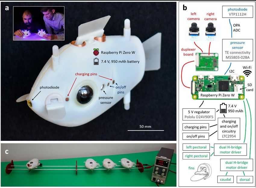
Fig. S20. Schematic of the tank view as seen from the overhead camera.

Other Supplementary Material for this manuscript includes the following:

(available at robotics.sciencemag.org/cgi/content/full/6/50/eabd8668/DC1)

 Movie S1 (.mp4 format). Introduction to Blueswarm.
 Movie S2 (.mp4 format). Collective organization in time.
 Movie S3 (.mp4 format). Collective organization in space.
 Movie S4 (.mp4 format). Dynamic circle formation.
 Movie S5 (.mp4 format). Multibehavior search operation.
 Movie S6 (.mp4 format). Summary and highlights.

Supplementary Material

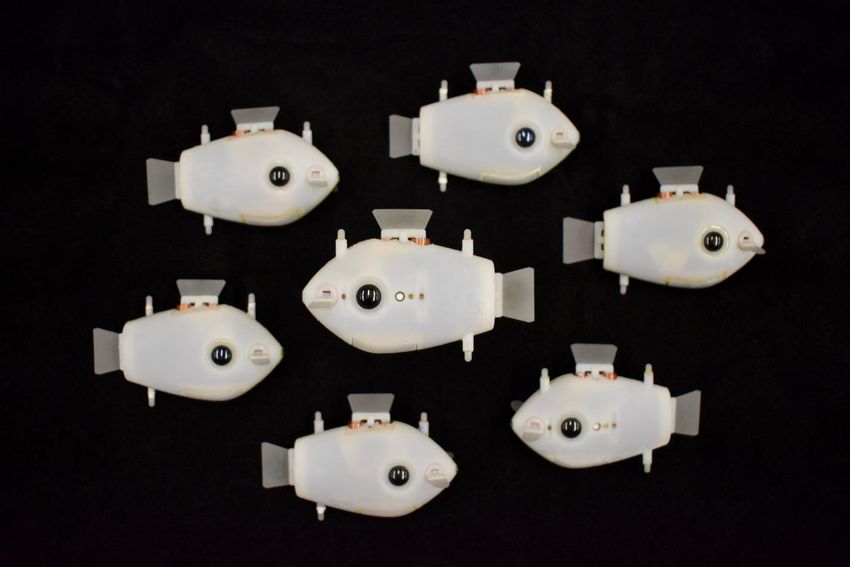
Table of Contents
1 The Bluebot 3D Vision System ........................................................................................ 3
 1.1 Overall Specifications .........................................................................................................3
 1.2 Neighbor Detection Algorithms ..........................................................................................4
 1.2.1 Camera Calibration ................................................................................................................................4
 1.2.2 Blob Detection .......................................................................................................................................4
 1.2.3 Camera Rotation Compensation and Coordinate Transformations ......................................................7
 1.2.4 From Blobs to Neighbors .......................................................................................................................8
 1.2.5 Neighbor Position Inference ..................................................................................................................9
 1.3 Vision System Accuracy .................................................................................................... 10
2 Controlled Dispersion ................................................................................................... 13
 2.1 Inter-robot Distances ....................................................................................................... 13
 2.2 Number of Visible Neighbors ............................................................................................ 15
 2.3 The Effect of Target Distance and Number of Robots on Dispersion ................................... 18
3 Dynamic Circle Formation and Milling .......................................................................... 20
 3.1 Overview of Theoretical Results ....................................................................................... 21
 3.2 Milling with Line-of-Sight Sensors ..................................................................................... 22
 3.2.1 Steady-State Milling Formation and Milling Radius .............................................................................22
 3.2.2 Unique Steady-State Configuration .....................................................................................................23
 3.2.3 Effects of 0 and 1 on Milling Formation ..........................................................................................24
 3.2.4 Lower-bound on the Sensing Range ....................................................................................................26
 3.3 Milling with Field-of-View Sensors.................................................................................... 26
 3.3.1 Milling Radius.......................................................................................................................................28
 3.3.2 Maximum Field of View .......................................................................................................................28
 3.3.3 Lower-bound on the Sensing Range ....................................................................................................29

4 Multi-behavior Search Experiments .............................................................................. 30
 4.1 Source Detection ............................................................................................................. 30
 4.2 Flash Detection ................................................................................................................ 31
 4.2.1 Challenges ............................................................................................................................................31
 4.2.2 Algorithm .............................................................................................................................................32

5 3D Tracking.................................................................................................................. 33
 5.1 Experimental Protocol...................................................................................................... 33
 5.2 Tracking ........................................................................................................................... 34
 5.2.1 Phase 1: Initialization ...........................................................................................................................34
 5.2.2 Phase 2: 2D Position Identification ......................................................................................................34
 5.2.3 Phase 3: 2D Trajectory Isolation ..........................................................................................................35
 5.2.4 Phase 4: 3D Data Fusion ......................................................................................................................36
 5.2.5 Phase 5: Post-Processing .....................................................................................................................39

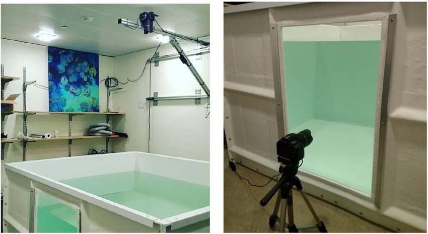
1 The Bluebot 3D vision system
The Bluebot’s vision system allows it to infer the presence and position of neighboring Bluebots
in a near 360 degree field of view, and to detect rudimentary signaling by other robots (see
Section 4.2). These capabilities enable 3D implicit coordination among Bluebots to achieve
collective behaviors in a Blueswarm.

1.1 Overall Specifications
The Bluebot’s vision system consists of two Raspberry Pi cameras1 interfaced to a Raspberry Pi
Zero W via a custom-built duplexer board. Each camera is equipped with a fish-eye lens with a
viewing angle of 195 degrees. The cameras are mounted on either side towards the front of the
robot, directly behind the pectoral fins. Each lens points outwards from the side but is angled
forward by 10 degrees. The lenses stick out from the hull of the robot to maximize the usable
field of view. Waterproofing is achieved by custom-built hemispheres made of clear plastic. The
two cameras combined give the Bluebot a quasi-omnidirectional field of view. There is some
overlap between the cameras’ fields of view at the front, while there is a small blind spot at the
back of the robot; see Figure 1 in the main paper for a scaled image of the FOV as well as a raw
image taken from the right eye of the robot. Here we show components and internal electronics
of Bluebot that were not labelled in the main paper (Figure S 1).

Figure S 1: Additional components of the Bluebot platform: (a) A photodiode, a pressure sensor, and pins for charging and
switching the robot on/off penetrate the body. (b) Sensors and actuators are internally connected to a Raspberry Pi Zero W
onboard computer. (c) Several Bluebots can be charged simultaneously on a custom charging rail.

1
 https://www.raspberrypi.org/products/camera-module-v2/

The Raspberry Pi camera is capable of taking still color images at a resolution of up to 2592 x
1944 pixels. However, the Raspberry Pi is not capable of performing image processing on images
of this size at a rate fast enough for real-time control. Therefore, the images are down sampled
to 256 x 192 pixels, most image processing is performed on the blue channel only, and significant
effort was put into the design of fast algorithms for neighbor position inference which are
described in the following subsections. Our final system led to a typical image capture and
processing cycle of around 0.5 seconds, meaning that the Bluebot can operate at a control cycle
of around 2 samples/second (allowing for image capture and processing from both cameras).
This control cycle is sufficiently fast compared to the relatively slow dynamics of the Bluebot,
which moves at speeds of less than 1 body length per second. We also measured the range and
accuracy of the cameras, reported in detail subsection 1.3. The robots are able to reliably detect
neighbors within 3 meters with highest accuracy in the front and sides (~80%), and lowest
accuracy (~75%) towards the back.

1.2 Neighbor Detection Algorithms
1.2.1 Camera Calibration
The Bluebot’s fisheye (spherical) lenses have a viewing angle of 195 degrees. This large viewing
angle comes at the cost of significant distortion in the image. Therefore, it is essential for the
cameras to be calibrated in order for a Bluebot to infer the relative positions of other Bluebots
from image data.

The calibration is achieved using the Omnidirectional Camera Calibration Toolbox2 for MATLAB
(OCamCalib), authored by Davide Scaramuzza. This toolbox provides a highly automated
calibration process. The user takes a number of images of a checkerboard pattern using the
camera to be calibrated. The software performs automatic checkerboard detection (asking the
user for help if necessary) and returns a number of calibration parameters. For a full explanation
of the calibration process and parameters, refer to the OCamCalib tutorial.

The calibration process returns a polynomial function for converting locations in the image (i.e.,
pixel coordinates) onto directions of rays in the real world (and vice versa, if desired). For a
camera system with no distortion, this function is simply a linear scaling, but the presence of
distortion requires a nonlinear function. For our particular camera and lens setup, a third order
polynomial yields the best results. In order to retain fast processing times, we only use this
polynomial on feature points of interest, and there is an additional step converting from camera
coordinate frame to robot body coordinate frame.

1.2.2 Blob Detection
A Bluebot detects the presence of other Bluebots by first locating their LEDs on its vision system.
The Bluebot’s camera settings (e.g., brightness, contrast) are set such that under lab experiment
conditions, everything in the images appears dark except for the LEDs of other Bluebots, which
are the brightest light sources in the environment. These settings facilitate the process of

2
 https://sites.google.com/site/scarabotix/ocamcalib-toolbox

detecting LEDs from other Bluebots, because they appear as more or less circular blobs in the
image. The process of detecting contiguous sets of pixels in an image is often referred to as blob
detection; in order to achieve fast processing times, we designed a simple custom algorithm
described below.

Our blob detection process starts by thresholding the image to obtain a binary image with only
black and white pixels. The threshold is set heuristically to achieve a balance between sensing
range and sensitivity to false-positive errors. We define blobs as continuous regions of white
pixels in a binary image. The notion of continuity depends on how neighbor pixels are defined.
Common definitions include 4-connectivity and 8-connectivity. We use the definition that two
pixels are connected if their Moore distance is smaller than or equal to two. This allows for gaps
of size one pixel within a blob.

Many algorithms exist for blob detection. A simple but effective method is to search for blobs via
a depth- or breadth-first search starting from every unvisited white pixel; this method will
correctly identify all blobs in every case. However, the Raspberry Pi zero’s limited computational
power renders this method too slow to be useful for real-time control on the Bluebots, even at
the reduced image resolution of 256 x 192 pixels.

We therefore opt for a trade-off with an algorithm that runs an order of magnitude faster but is
not guaranteed to identify all blobs in every case, as we will discuss. In practice, our successful
experiments demonstrate that this detection system is sufficient. The algorithm is based on
identifying continuous pixels first in one direction and then in the other, and inherently considers
pixels to be connected or not according to their Moore distance. We introduce a parameter 
that defines the maximum Moore distance for two pixels to be considers connected. Setting =
1 reduces to 8-connectivity and increasing allows for some black pixels within blobs.

The blob detection algorithm proceeds as follows:

 i. Store all white pixels in a list, recording their ( , ) coordinates.
 ii. Sort the white pixels by coordinate.
 iii. Split this sorted list into sub-lists wherever there is a gap larger than between successive
 coordinates.
 iv. For each of these sub-lists:
 a. Sort the pixels by coordinate.
 b. Split this sorted list into sub-lists wherever there is a gap larger than between
 successive coordinates.
 c. Each sub-list now corresponds to a blob. Calculate its centroid and add it to the
 list of blob centroids.
 v. Return the list of blob centroids.

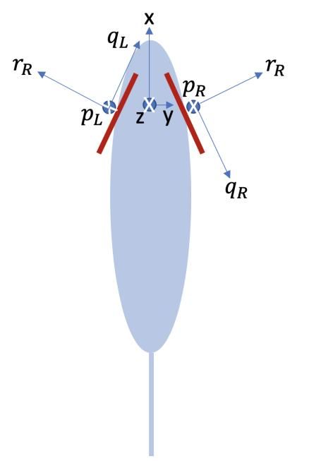
Figure S 2: Example scenarios for the blob detection algorithm: (a) Non-pathological; (b, c) Pathological

Correctness
In the following analyses, we assume = 1 for a simplicity. Figure S 2a shows a non-pathological
case for the blob detection algorithm. In Step (iii), blobs C and D are isolated, but blobs A and B
are grouped together because their (i.e., horizontal) coordinates overlap. Blobs A and B are
then separated in Step (iv.b), because their coordinates are not continuous.

Figure S 2b shows the first pathological case for the blob detection algorithm. In the coordinate
pass of Step (iii), all three blobs are added to the same sub-list because their coordinates are
continuous. In Step (iv.b), blob B is isolated, but blobs A and C remain lumped together because
their coordinates are continuous. This pathological case can be solved by recursively calling the
algorithm on all sub-lists after Step (iv.b): once blob C is removed, blobs A and B are distinguished
by another pass of the algorithm. In general, the algorithm would have to be called recursively in
Step (iv.b) whenever any splits are made in Step (iv.a). We opt not to use this recursion in our
implementation, because it slows down the algorithm significantly and does not provide a
substantial benefit in practice. Even if recursion is used, there are still some pathological cases
that cannot be resolved by this algorithm, as shown in Figure S 2c. These two blobs will always
be identified as one because they are continuous in both and coordinates. Given the circular
nature of the LEDs, we do not expect many pathological cases to arise. In addition, in our practical
setting we have many more sources of error and noise, e.g. reflections and occlusions, that play
a more significant role in reducing the accuracy of neighbor detection.

Time complexity
Depth and breath-first searches visit every node and edge in a graph exactly once. Here, an image
has nodes (pixels), and ( − 1) + ( − 1) edges (links between adjacent pixels). The

 6

resulting time complexity of depth-first search (DFS) is O(3 ), regardless of how many white
LED blob pixels there are in any given image.

Figure S 3: Time complexity of rapid LED blob detection at an image resolution of 256 x 192: (a) A typical image taken with a
Bluebot during aggregation with seven robots, which contains 0.35% white pixels. (b) Rapid LED blob detection (RapidLED) is
significantly faster than depth-first search for low ratios of white LED blob pixels in a given image. The ratio of white pixels in
Bluebot images typically falls into the yellow left region. RapidLED would process example image (a) with approximately 2.9 fewer
computational steps than DFS.

Our blob detection process (RapidLED) also visits all pixels once to identify white pixels above
a heuristically tuned threshold (Step (i) in the above blob detection algorithm). Let's denote the
ratio of white pixels in an image as (e.g., an image with = 0.005 contains 0.5% white pixels).
For each of Steps (ii) and (iv.a), RapidLED has to sort at most pixels total, and sorting takes
time O( log( )). The resulting time complexity of RapidLED is O( +
2 log( )), and depends on the ratio of white pixels in any given image.

Figure S 3B shows the number of computational steps required for different ratios of white pixels
for a Bluebot image of size 256 x 192. As long as there are fewer than 11.6% white pixels,
RapidLED requires fewer steps than DFS. Typical Bluebot images have less than 1% white pixels
(yellow left region), and are processed significantly more efficiently with RapidLED (e.g., 2.9 times
fewer computational steps for the image in Figure S 3A). The mean and standard deviation of
white pixels taken from 453 images over the course of a representative dispersion-aggregation
experiment were = 0.27% and = 0.26%, respectively. At most, there were 1.86% white
pixels in an image showing a very nearby robot, and only 14 images out of 453 had more than 1%
white pixels.

1.2.3 Camera Rotation Compensation and Coordinate Transformations
The next phase in vision processing after blob detection is to convert blob locations in the images
given in ( , ) coordinates into directions in the robot coordinates ( , , ). Figure S 4 shows the
camera world coordinate systems and the robot coordinate system. The subscripts and in
the camera world coordinate systems stand for “Left” and “Right” respectively. The cameras on
the Bluebot are mounted towards the front on either side (2.5 cm from body center) and inclined
forward by an angle of 10 degrees.

 

Figure S 4: Camera and robot coordinate systems.

The first step is to transform each blob coordinate ( , ) into a direction ( , , ) in its camera’s
world frame. This is achieved using the calibration function (see Section 1.2). The points ( , , )
are then transformed into robot coordinates ( , , ). For the left camera, a counterclockwise
rotation of 10 degrees around the axis is first applied, and then the following coordinate
transformation is applied:

 = 
 = − 
 = − 

For the right camera, a clockwise rotation around the axis is first applied, and then the
following coordinate transformation is applied:

 = − 
 = 
 = − 

Note that the small translations between the camera world coordinate frames and the robot
coordinate frame are negligible and therefore ignored for simplicity. All the identified blobs are
now available in robot coordinates ( , , ).

1.2.4 From Blobs to Neighbors
Identifying the number of neighbors requires pairing blobs to individual robots. For most robots,
the two LEDs produce two nearby blobs, however for some robots only one blob (or none) may
be visible due to occlusion, and there may be spurious blobs due to surface reflections. We call

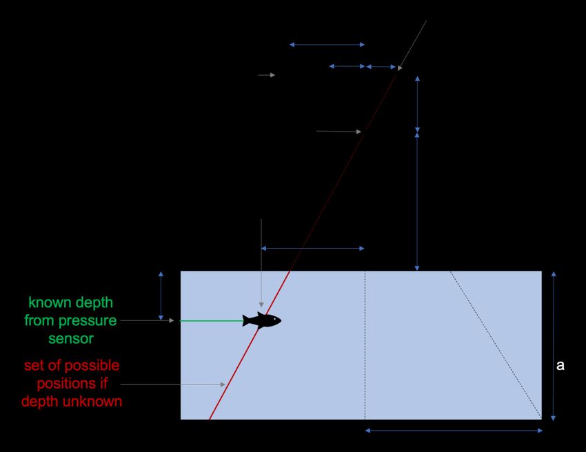
the procedure of pairing blobs and identifying spurious blobs blob parsing. Once pairs of blobs
have been assigned to individual robots, it is then possible to estimate the distance to those
robots, which is the subject of the next section.

The criterion used for blob parsing is that pairs of blobs belonging to the same Bluebot must be
vertically aligned, because the Bluebots are designed to be passively stable in roll and pitch. There
are several ways to address the blob parsing problem. In general, it may be framed as a
combinatorial optimization problem and then approached using general solvers. For the
purposes of this work, it was sufficient to use simple heuristics to obtain reasonably good blob
parsing. Reflections are eliminated by considering the location of the water surface from the
Bluebot’s known depth and discarding any blobs above this level. Pairing is achieved by
considering the best-matched pair of blobs in terms of vertical alignment and accepting them as
a single Bluebot if their vertical alignment is better than a predefined, fixed threshold. The second
best-matched pair are then considered, and so on as long as pairs of blobs are available that are
vertically aligned within the threshold. Blobs that do not get paired within the set threshold are
discarded for parsing purposes but can still provide useful information in certain algorithms (e.g.,
ones that only care about bearings to neighbors).

In general, it is also possible to modify the Bluebot design and operational protocol to introduce
additional criteria that may make blob parsing easier. For instance, the two LEDs on a Bluebot
could have different colors. Alternatively, Bluebots could flash their LEDs intermittently rather
than leave them on continuously – this way, pairs of LEDs belonging to the same Bluebot would
be more likely to appear locally isolated. However, these techniques introduce additional
challenges, and in this work, we limit ourselves to the basic scenario with two identically colored,
continuously on LEDs.

1.2.5 Neighbor Position Inference
We are given two blobs in the robot coordinate frame that correspond to the same neighboring
Bluebot: ( 1 , 1 , 1 ) and ( 2 , 2 , 2 ). Without loss of generality let 1 > 2 so that 1 corresponds
to the Bluebot’s lower LED. Recall that these two vectors are unit vectors and represent only the
directions of the LEDs in the robot’s local coordinate frame. However, since we know the vertical
distance Δ between LEDs on the Bluebot, we can infer the distance to this Bluebot.

Let ( , , ) represent the position of the Bluebot’s lower LED in the world coordinate frame.
Then, the upper LED’s position is ( , , + Δ). Furthermore, we have that:

 ( , , ) = ( 1 , 1 , 1 )
 ( , , + Δ) = ( 2 , 2 , 2 )

for some scalars and , which are the distances we need to solve for.
We have = 1 and = 2 , from which:
 1
 = 
 2

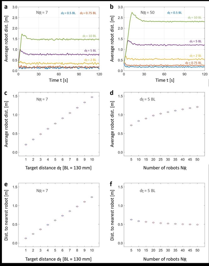
Similarly, we have = 1 and = 2 , from which:
 1
 = 
 2

Under ideal conditions, we should have:
 1 1
 =
 2 2

but in general, this may not be true due to noise in the blob detection process. In practice, we
may take the average value of 1 / 2 and 1 / 2 , but for simplicity here we will opt for 1 / 2 as
the true value.

We also have:
 = 1
 + Δ = 2

or, combining:
 1 + Δ = 2
 
Substituting = 1 and rearranging, we obtain:
 2
 Δ 2
 =
 1 2 − 2 1

which is the distance to the Bluebot’s lower LED.

1.3 Vision System Accuracy
To evaluate the accuracy of the Bluebot’s vision system, we performed a series of tests. One
Bluebot (A) was placed in a fixed position and programmed to infer the position of another
Bluebot (B). Bluebot B was placed in various positions relative to A, namely in all possible
combinations of:

 i. Distance: 0.5 m, 1.0 m, 1.5 m, 2.0 m, 2.5 m, 3.0 m
 ii. Planar Bearing: 0 deg., 45 deg., 90 deg., 135 deg.
 iii. Height: 0.0 m, 0.5 m, 1.0 m

This gives a total of 6 x 4 x 3 = 72 measurements. Here we present the results for the case where
the height is 0.0 m as the other heights gave similar results.

Figure S 5 shows the position estimation error along the and directions. Blue dots represent
the ground truth (i.e., the actual position of Bluebot B) while red dots represent Bluebot A’s
estimate of Bluebot B’s position. The error grows slightly with distance for all angles, but is within
20% even at a distance of 3.0 m.

Figure S 6 shows the error along the direction as a percentage of the distance between the
Bluebots. The error depends on the angle, but levels off at a maximum of 15%.

Finally, Figure S 7 shows the overall error as a percentage of distance . The overall error is
defined as:

 Δx 2 Δy 2 Δz 2
 √
 = 100 ∗ ( ) + ( ) + ( )
 
Our overall results show that the error for a single neighbor robot position depends on the angle
more than it does on the distance, and the error levels off at around 20% in the best-case scenario
and 25% in the worst-case scenario.

Figure S 5: x and y error in the Bluebot's position estimation for 24 cases. Blue dots represent the ground truth while red dots
represent the inferred position.

Figure S 6: Error in the z direction as a percentage of distance. Colors represent different angles (see legend).

Figure S 7: Overall (x,y,z) error as a function of distance. Colors represent different angles (see legend).

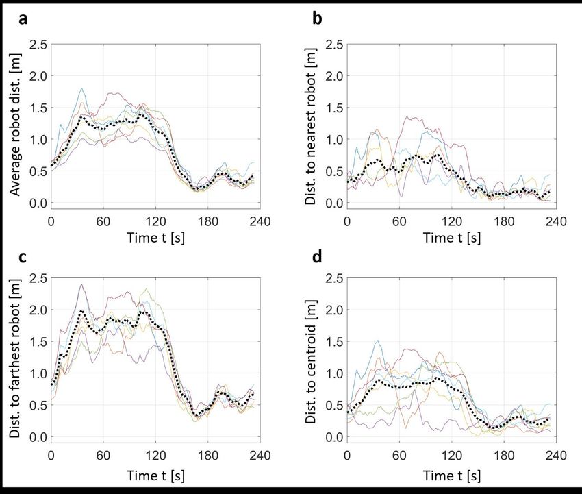
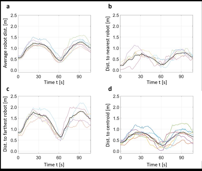
2 Controlled dispersion
Bluebots control their collective spread through decentralized attractive and repulsive virtual
forces. The collective is capable of changing the volume it covers up to eightyfold in our
laboratory environment (Figure 3 in the main paper). Here we provide additional analyses of the
dispersion behavior, including a detailed investigation of inter-robot distances (Section 2.1) and
the number of visible neighbors over the course of an experiment (Section 2.2). In addition, we
present scaling intuition on the collective spread influenced by the inter-robot target distance
and the number of participating robots from an idealized 3D point-mass simulation (Section 2.3).

2.1 Inter-robot Distances
We ran two types of experiments on dispersion with the same inter-robot target distances of 2
body lengths for the dispersed and 0.75 body lengths for the aggregated state, respectively. In a
first experiment, seven Bluebots dispersed for 120 seconds followed by aggregation for another
120 seconds (Figure S 8).

Bluebots were able to hold the average distance to neighboring robots relatively constant (Figure
S 8a). The differences in measured average distances among the robots are expected, and larger
in dispersed (~50 s – 100 s) than aggregated (~170 s – 230 s) state (Figure S 8a): a robot positioned
around the center should have a lower average distance to neighbors compared to another robot
at the periphery. In contrast, the distance to a single nearest neighboring robot (NND) fluctuated
considerably, especially during dispersion (Figure S 8b). This shows that Bluebots continuously
adjusted their positions in an effort to minimize the virtual forces acting on them, whereby the
nearest neighbor is more likely to exert a strong force than far away neighbors. The distance to
a single farthest robot (Figure S 8c) is generally larger than to the nearest robot (as expected),
and within the longest dimension (2.97 m) of our test bed. Finally, the distances of all robots to
their momentary collective centroid demonstrates that they spread out effectively during
dispersion (with some robots close and some far from the centroid), and reduced this spread
during aggregation (Figure S 8d).

In a second experiment, seven Bluebots dispersed and aggregated repeatedly during four 30
second long intervals (Figure S 9). Similar observations can be made as for the first experiment.
The average distances during dispersion and aggregation peaks are comparable between the two
experiments: approximately 1.2 m and 0.5 m in Figure S 9a versus 1.3 m and 0.4 m in Figure S 8a.
The dynamic switching between dispersion and aggregation (Figure S 9a-c) appears to yield
marginally more uniform inter-robot distances than programming robots to hold dispersion and
aggregation for prolonged durations (Figure S 8a-c).

Figure S 8: Interrobot distances during single dispersion/aggregation: (a) average distance to all neighboring robots; (b) distance
to the nearest neighboring robot (NND); (c) distance to the farthest neighboring robot (NND); (d) distance to the momentary
centroid of all robots. Colored solid lines represent individual robots; the black dashed line represent the average of the seven-
robot collective.

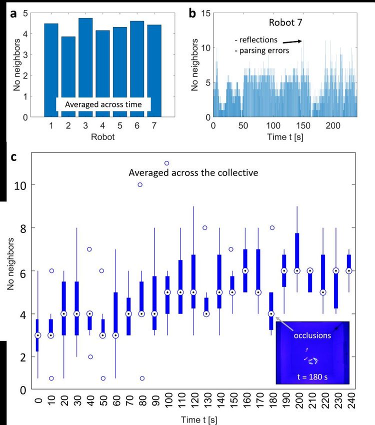
Figure S 9: Interrobot distances during repeated dispersion/aggregation: (a) average distance to all neighboring robots; (b)
distance to the nearest neighboring robot (NND); (c) distance to the farthest neighboring robot (NND); (d) distance to the
momentary centroid of all robots. Colored solid lines represent individual robots; the black dashed line represent the average of
the seven-robot collective.

2.2 Number of Visible Neighbors
During dispersion, Bluebots estimate the distances to their visible neighbors from pairs of
vertically stacked LEDs they believe to belong to individual robots (Section 1.2.5). This estimation
is noisy by nature of the visual system (Section 1.3), but more drastic errors are introduced when
the parsing algorithm mistakenly assumes two LEDs to belong together and represent a fellow
robot. Furthermore, neighboring robots may not be seen at all due to occlusions, and occasional
“ghost robots” appear when surface reflections of LEDs are not filtered out correctly.

During the first experiment on controlled dispersion (Figure 3F in the main paper), Bluebots
dispersed for 120 s and aggregated for the next 120 s. From their onboard log files, we know how
many neighbors they believed to see in each iteration. 8287 neighbor counts were made by all
robots over the time of the entire experiment. On average, individual robots saw between 3.9
and 4.7 neighbors during the experiment (Figure S 10a); in the ideal case each robot would see

all 6 neighbors at all times. The collective median was lower during dispersion (4.2) than
aggregation (5.6), most likely because more robots were hidden in the blind spots (Figure S 10c).

921 neighbor counts (11% of all counts) were greater than 6, i.e. impossible since there were only
7 robots total (see Figure S 10b for such instances). 11% is a lower bound for over-counting, since
other counts might also include mistaken neighbor identifications. The main reason for over-
counts is incorrectly handled surface reflections leading to “ghost robots”. Such reflections
always appear higher up than the actual robots. As a consequence, over-counts introduce two
systematic biases:

 i. Robots aggregate at the surface, since over-counts appear high up and exert an additional
 attractive force toward the surface.

 ii. Over-counts magnify the z-component (depth) of dispersion (but not for robots that
 remain at the surface and do not see over-counts).

Despite these shortcomings, the overall density of the collective could be controlled effectively,
and a large volume change could be achieved by changing the target distance parameter.

Figure S 10: Number of visible robots during controlled dispersion: (a) for each of N = 7 robots, averaged across time; (b) for robot
7 at each sampling iteration; (c) for each of 25 equally spaced instances in time, averaged across the collective of N = 7 robots,
showing the median, 25th and 75th percentiles, most extreme data points, and outliers.

2.3 The Effect of Target Distance and Number of Robots on Dispersion
We ran idealized 3D point-mass simulations to study the effect of the target distance and the
number of robots on dispersion. The simulations assumed holonomic point-mass robots with
omnidirectional perfect vision and constant speed locomotion (1 Bluebot body length per
iteration). In this idealized simulation, the environment was unbounded, and the number of
robots could be varied easily, as opposed to our physical experiments in a water tank.

Overall, the simulation results show that the resultant average distance between robots grows
with the prescribed target distance dt, and also with the number of robots NR in the collective
(Figure S 11a-d). The distance to the single nearest neighboring robot (NND) grows linearly with
the target distance as well, but tends to plateau with the number of robots (Figure S 11e-f).
Therefore, the target distance is an effective predictor and control parameter for NND, regardless
of the number of robots in the collective. From the linear scalings between the average robot
distance and target distance, as well as NND and target distance (Figure S 11c,e), we conclude
that it should be theoretically possible to accurately control the spread of a robot collective with
the potential-based dispersion protocol used in our real robot experiments.

There is a gap between theory and practice however: in simulation, seven robots spread to
average distances of approximately 0.2 m and 0.34 m for dt = 0.75 body lengths (BL) and dt = 2
BL, respectively (Figure S 11c), while in practice 0.4 m and 1.3 m were measured for the same dt
= 0.75 BL and dt = 2 BL (Figure S 8a). Two differences between simulations and real robot
experiments that could potentially explain this discrepancy are:

 i. The robots in simulation have perfect vision and see all neighbors at all times, while the
 real robots do see a limited number of neighbors only (Section 2.2). Because of occlusions,
 it is more likely that the real robots see close than distant neighbors. This may bias the
 virtual forces toward repulsion and trigger larger than theoretically predicted dispersion.

 ii. The robots in simulation move at constant speed, while the real robots adjust their speeds
 (or fin frequencies, respectively) according to the magnitude of the net virtual force.
 Because of the non-linear nature of the potential-based virtual forces, repulsive forces
 are much stronger than attractive forces. The mapping from attractive net forces to fin
 frequencies to robot speeds may have been too weak to produce sufficiently strong
 aggregation in real robot experiments.

The Lennard-Jones potential is one of many possible controlled dispersion potential functions.
The above limitations could be addressed by selecting a different potential function that weighs
attractive forces more heavily, and/or enforcing a minimum robot speed even at very low net
forces. Although the dispersive effects are greater in the Blueswarm, this does not prevent the
collective from effectively aggregating and repeatedly switch between aggregated and
dispersed states. Future experimental comparison of multiple dispersion algorithms can lead to
a deeper understanding of practical issues and theory-realization gaps.

Figure S 11: Target distance and number of robots influence interrobot distances during dispersion: (a) the resultant average
distance between NR = 7 robots grows with the prescribed target distance dt; (b) the average distance between NR = 50 robots is
larger than for NR = 7 robots; (c) the simulation runs are repeatable and indicate a linear scaling between the average robot
distance and the target distance (BL = body length) for a fixed number of NR = 7 robots; (d) the average robot distance also grows
with NR for a fixed dt = 5 BL; (e) moreover, the distance to the nearest neighboring robot (NND) grows linearly with dt; (f) however,
NND does not grow with NR. Subfigures (a,b) show the time series of a single experiment; (c-f) show the means (red circles) and
standard deviations (blue lines) from N = 10 simulation runs per data point.

3 Dynamic circle formation and milling
The dynamic circle formation and milling algorithm used in this paper places strikingly few
requirements on the part of the robots. In particular, it is only assumed that:

 o Each robot has a line-of-sight or a field-of-view binary sensor that can detect the presence
 of other robots. The sensor returns 0 if it does not detect other robots and 1 if it does.
 The robot does not need to know the number or exact positions of robots within the field-
 of-view, thus placing very little load on the neighbor parsing accuracy and working with
 minimal information.

 o The robots are capable of moving in a planar circle of a fixed radius at a fixed speed in
 either direction (i.e., clockwise or counterclockwise). For dynamic cylinder formation, we
 also assume that robots can independently control their depth in the tank while moving
 clockwise or counterclockwise in the plane.

The algorithm itself is also extremely simple. Each robot follows the following protocol:

 o If the sensor returns 0, rotate clockwise3 along a circle of radius 0 with a fixed speed.
 o If the sensor returns 1, rotate counterclockwise along a circle of radius 1 with a fixed
 speed.

Previous work in simulated ground robots suggested that this algorithm generates an emergent
rotating circle formation, where ideal robots (with no sensory or locomotion noise) are equally
distributed along the circle and the size of the circle increases with the number of the robots 4.

Here we prove that the original algorithm for simulated ground robots with line-of-sight sensors
has a unique stable state with a circle radius R whose formula is derived, and we also provide
bounds on necessary parameters to achieve stable configuration. By stable, we mean that the
robot formation will never change (except for the robots rotating indefinitely). We then extend
this proof to the Bluebots which use an angular field-of-view sensor.

In the following analysis, we make several simplifications:

 o The sensor-actuator loop is fast enough that it can be considered continuous.

 o There is no noise on the robots’ sensor readings and locomotion.

3
 The words clockwise and counterclockwise in the algorithm can be freely interchanged, as long as the robots rotate
in opposite directions in the cases where they do or do not see other robots. The milling occurs in the direction that
the robots rotate when they do not see another robot (i.e., when the sensor reads 0). In the following we assume
that milling occurs in a clockwise direction.
4
 M. Gauci, J. Chen, W. Li, T. J. Dodd, and R. Groß, “Self-Organized Aggregation Without Computation,” International
Journal of Robotics Research, vol. 33, no. 8, pp. 1145–1161, 2014.

o The robots have no inertia and can change directions (i.e., from rotating clockwise to
 counterclockwise or vice versa) instantaneously. This simplification does not hold strongly
 for the Bluebots, but it makes the analysis tractable, and simulation and physical results
 show that milling with the Bluebots is indeed possible.

 o The robots are on the same horizontal plane. This simplification leads to no loss of
 generality as long as the robots’ sensors are implemented in such a way that they are
 invariant to other robots’ altitudes/depths.

3.1 Overview of Theoretical Results
In this section we introduce the main parameters and present a short overview of the theorems
and insights that will follow in more detail in the subsequent sections.

We are given a number of robots and assume that the robots have an approximately circular
body of radius (for the purposes of being sensed by other robots). We begin by considering
line-of-sight sensors, which will then easily extend to the more general case of field-of-view
sensors.

Given and , we show that there is a unique stable milling configuration with radius:

 =
 2 
 1 − cos 

provided certain conditions are satisfied, namely:

 o The robots’ turning radius when the sensor reports no other robots, 0 , must be smaller
 than or equal to the milling radius: 0 ≤ . Milling is smoother if the two values are
 similar, i.e., if 0 is not much smaller than .

 o The robots’ sensors must have sufficient range, and a lower-bound on this sensing range
 is theoretically calculated.

We then generalize the above results to the case of a field-of-view sensor. The sensor’s half field
of view is denoted by . The line-of-sight sensor results are all recoverable from the field-of-view
sensor results by setting = 0.

 ′ =
 2 
 cos − cos ( − )

For a field-of-view sensor, the milling radius now depends on , , and . The same conditions
as for line-of-sight sensors still hold, but the lower-bound on the required sensing range now also
depends on . Additionally, there is also a theoretically calculated upper-bound on to achieve
a finite steady-state milling radius. For values of larger than this upper-bound, the milling radius

grows until the robots can no longer see each other (or indefinitely if the sensing range is
unlimited).

In the following subsections, we provide proofs for each of the claims made above.

3.2 Milling with Line-of-Sight Sensors
3.2.1 Steady-State Milling Formation and Milling Radius
The first theorem shows that a milling formation can be maintained if starting from an idealized
configuration and with an optimal choice of 0 .

Theorem 1. Given a free choice of 0 , robots of radius can be placed on the vertices of a
regular -sided polygon such that upon moving, no robot detects another robot, and the polygon
formation is maintained indefinitely. The radius of this polygon is:

 =
 2 
 1 − cos 

and we choose 0 = .

Figure S 12: Seven robots arranged in a regular polygonal formation with line-of-sight sensors tangential to each other.

Proof. Consider the configuration in Figure S 12, where robots are placed on the vertices of a
regular -sided polygon and each robot is oriented such that its sensor is tangential to the

subsequent robot. In this configuration, no robot detects another robot. Now, if the robots rotate
clockwise with the same radius as the radius of the polygon (i.e. 0 = , as shown by the dotted
circle), we have the invariant property that no robot will ever see another robot as they move. It
remains to calculate the radius of the polygon, .

Figure S 13: Expanded view of the red quadrilateral in fig. S 12.

Figure S 13 shows an expanded view of the red quadrilateral in Figure S 12. Since the polygon is
regular, the angle spanning from the center of the polygon to any two adjacent robots is given
by = 2 / . Observe from the triangle in Figure S 13 that:

 2 − 
 cos =
 
which can be rearranged to give:

 =
 2 
 1 − cos 

This concludes the proof. QED.

3.2.2 Unique Steady-State Configuration
To the best of our knowledge, we do not know of a method to prove or guarantee the
convergence of this minimalist binary sensing approach to the milling formation, starting from
an arbitrary initial configuration of robots5. However, assuming an unlimited sensing range and

5
 Stabilization guarantees have been found for other decentralized circular formation algorithms with various spacing
patterns (e.g., equidistant milling) for point-mass particles that use omnidirectional active communication:
 - Sepulchre, R., Paley, D. A., & Leonard, N. E. (2007). Stabilization of planar collective motion: All-to-all
 communication. IEEE Transactions on Automatic Control, 52(5), 811–824.
 - Sepulchre, R., Paley, D. A., & Leonard, N. E. (2008). Stabilization of planar collective motion with limited
 communication. IEEE Transactions on Automatic Control, 53(3), 706–719.

 0 = , it is easy to show that the milling formation of Figure S 12 is the only stable formation.
By stable, we mean that no robot will ever see another robot, and therefore the formation will
never change (except for the robots rotating indefinitely).

Theorem 2: The regular polygon formation of Theorem 1 is the unique stable formation if the
sensing range is unlimited and 0 = .

Proof. In Figure S 14, robot A rotates along a circle of radius 0 = . For contradiction, assume a
formation not identical to the one of Theorem 1. Then, at least one other robot, say robot B, does
not have its center lying on the circle traversed by robot A. Therefore, robot B traverses a circle
different to the one traversed by robot A. It is clear that as both robots move along their
respective circles, each robot’s sensor must at some point intersect the other robot. Thus, the
configuration is not stable. QED.

Figure S 14: Example configuration of two robots to show that the regular polygon formation of Theorem 1 is the only stable
formation.

Previous work’s simulation results, and our own MATLAB simulations, suggest that the stable
milling formation in Figure S 12 with the corresponding milling radius, is achieved from any initial
configuration with 0 = , even though a proof of convergence does not yet exist. Furthermore,
these simulation results suggest that this algorithm works for 0 ≤ and with sufficient (not just
unlimited) sensing range. These two conditions are expanded on in the following two sections.

3.2.3 Effects of 0 and 1 on Milling Formation
Theorems 1 and 2 assume that 0 , the turning radius of the robots when their sensor reads 0, is
equal to the milling radius . Under this condition, no robot in the formation will ever see another
robot, and the formation is maintained indefinitely. In practice, this is achievable if the number
of robots is known and the turning radius is easily adjustable, but it is not possible if the turning
radius is fixed and the number of robots is unknown or variable.

To examine the effect on 0 on maintaining the formation in Figure S 12, consider one of the
robots and consider its position after a short amount of time . If 0 = , then the robot’s center
will still be on the dotted circle, only shifted slightly clockwise. Moreover, its sensor will still be
tangential to the next robot, and therefore its sensor will still read 0 and it will continue rotating
clockwise.

Assume now that 0 < . The robot’s center after a short period of time will now lie slightly
inside the dotted circle, and as a result, its sensor will now intersect with the next robot, returning
a reading of 1. As a result, the robot will now rotate counterclockwise with radius 1. This creates
a negative feedback mechanism that, on average, maintains the formation of Figure S 12.
Naturally, the closer 0 is to the more smoothly the formation can be maintained, but
simulation results show that 0 can be reduced by around an order of magnitude before any
noticeable deviations start to occur, and by around two orders of magnitude before the overall
formation is seriously compromised. Simulation results also show that setting 1 = 0 in all cases
is a reasonable choice.

Assume that 0 > . In this case, we can guarantee that it is not possible to achieve the formation
of Figure S 12 starting from any initial configuration (but it might be possible starting from some
initial configurations). We state this as a theorem.

Theorem 3. If 0 > , it cannot be guaranteed that the robots will converge to a regular polygon
of radius .

Proof. We prove this statement by providing a pathological initial configuration. We only need to
redraw the formation of Figure S 12, but with replaced by 0 and some of the robots removed,
as shown in Figure S 15.

Figure S 15: A pathological initial configuration for the case _0 > 

None of the five robots see each other, and therefore they will continue rotating along the circle
of radius 0 , never converging to a regular pentagon. QED.

The above analysis, coupled with simulation results, suggest that in practice it is advisable to set:

 < 0 < 
 10

 1 = 0

3.2.4 Lower-bound on the Sensing Range
If 0 = , the robots in Figure S 12 will maintain their formation regardless of the sensing range,
because no robot will ever see another robot in any case. However, if 0 < , then maintaining
the formation relies on the negative feedback effect discussed in the previous section, which
relies on each robot being able to sense the adjacent robot. Therefore, a lower-bound on the
sensing range required to maintain the formation is given by calculating the value of in Figure
S 13. We see that:

 2 
 = sin
 
or, substituting in the expression for calculated in Theorem 1:

 2 
 sin 
 =
 2 
 1 − cos 

Note that this is only a lower-bound on the required sensing range and does not say anything on
the ability of robots being able to form the milling formation from any initial configuration. The
ability to form the milling formation depends on the compactness of the initial configuration. We
do not yet have a method to guarantee convergence of our algorithm to the milling formation
from arbitrary initial configurations, but simulation results suggest that milling is almost always
successful if the robots initially form a strongly-connected graph (with two robots being
connected if they are within each other’s sensing range).

3.3 Milling with Field-of-View Sensors
In this section we generalize the results of the previous section to the case of a field-of-view
sensor. In practice, field-of-view sensors are more practical to implement than line-of-sight
sensors (strictly speaking, even a column of width 1 pixel corresponds to a field-of view).
Moreover, having a field of view allows us to control the radius of the formation. The only two
results that must be modified are the milling radius in Theorem 1 and the lower-bound on the
sensing range in Section 3.2.4.

Recall that we define as the half field of view of the sensor to obtain simpler equations, but for
brevity we refer to it as the field of view.

Figure S 16: A regular polygon configuration with field-of-view sensors (cf. fig. S 12 for line-of-sight sensors). Only two robots
are shown for simplicity; additional robots lie on each vertex of the polygon.

Figure S 12 must be modified to account for the field of view. The resulting configuration is shown
in Figure S 16 (only two robots are shown for simplicity; additional robots lie on each vertex of
the polygon).

Figure S 17: Geometry for calculating the milling radius with field-of-view sensors.

3.3.1 Milling Radius
Figure S 17 shows an expanded view of the red quadrilateral in Figure S 16, with additional
annotations and measurements. The additional measurements follow from the ones in Figure S
16 by simple geometrical observations. Note that we have defined = 2 / to keep the
equations simpler.

Now, referring to the uppermost triangle in Figure S 17, we have:

 sin − cos − cos 
 tan = =
 cos sin + sin 

which can be rearranged to give:

 =
 cos − cos cos − sin sin 

The denominator can be further simplified via trigonometric identities, and reintroducing =
2 / we finally obtain:

Equation 1

 =
 2 
 cos − cos ( − )

As a check, observe that letting = 0 in the above equation, we recover the equation for the
line-of-sight sensor given in Theorem 1.

3.3.2 Maximum Field of View
Theorem 4. The maximum field of view for achieving a finite-radius, steady-state milling
formation is = / .

Proof. Observe from Equation 1 for that the denominator tends to 0 as → ⁄ from below,
meaning that → ∞. For > / , we have < 0. In other words, the expression only provides
admissible (i.e. positive) values for when ∈ [0, / ]. QED.

The intuitive explanation of this result is that for a given number of robots, if the field of view is
set too large, the robots see each other more often than not and move counterclockwise,
effectively increasing the circle radius. Consequently, it becomes geometrically impossible to
form a finite-radius regular polygon formation where no robot sees another robot.

Simulation results show that if > / , a regular polygon formation is still formed, but its radius
grows indefinitely. This is because as robots see other robots, they rotate counterclockwise
making the formation larger.

3.3.3 Lower-bound on the Sensing Range
It is straightforward to calculate the lower-bound on the sensing range as we did for the case of
line-of-sight sensors (Section 3.2.4). In particular, we only need to apply the Pythagorean
theorem to the upper triangle in Figure S 17 to find the length of the hypotenuse :

 = √( − cos − cos )2 + ( sin + sin )2

4 Multibehavior search experiments
Section 1 explained the vision processing involved on a Bluebot for detecting the direction and
distance to other Bluebots. This vision processing is used on all the experiments, but the search
experiments make use of an additional two kinds of vision processing.

 o The Bluebots must be able to detect the source from close distance and differentiate it
 from other Bluebots. The source emits a red light as opposed to the blue light emitted by
 Bluebot LEDs.

 o The Bluebots must be able to detect flashing Bluebots and distinguish them from other
 Bluebots whose lights are continuously on.

4.1 Source Detection
Source detection works by comparing the red and blue channels of the image. For source
detection, blob detection is performed not only on the blue channel of the image, but on the
average of the channels (i.e., a greyscale version of the image).

After blob detection is performed, every blob larger than a predefined threshold is considered
a candidate to be the source. Blobs that are too small are not considered to avoid noise and to
make sure that Bluebots can only detect the source when they are sufficiently close to it. For
each candidate blob, the blue and red values of all the pixels within a Moore distance of the
blob’s centroid are summed up separately, and the ratio of the red total to the blue total is
calculated. A blob is considered to be red (i.e., the source), if this ratio is larger than some value.
We set = 3 and = 2, and the blob is considered red if the red-to-blue ratio is larger than
1.2.

We approximate the expected time for source detection if Bluebots do not collaborate with a
random walk of a single robot on an undirected graph . The vertices of are the integers 0, … , 
and represent distance to the source; consecutive vertices are connected. We calculate the
expected number of steps ℎ to reach the target node (the source) when starting from initial
node . We reach the source at vertex , so ℎ = 0; we can only move closer to the source from
vertex 0, so ℎ0 = ℎ1 + 1. For all intermediate vertices 1 ≤ ≤ − 1, we use linearity of
expectations to find ℎ . We introduce , a random variable for the number of steps to reach 
starting from . For a random walk, = −1 + 1 and = +1 + 1 are equally likely with
probability 1⁄2 each. Hence

 1 1
 [ ] = [ ( −1 + 1) + ( +1 + 1)] ,
 2 2

where [ ] = ℎ and by linearity of expectations, ℎ = ℎ −1 ⁄2 + ℎ +1 ⁄2 + 1. This gives us the
following system of equations:

 ℎ = 0,

ℎ −1 ℎ +1
 ℎ = + +1 ∀ 1 ≤ ≤ − 1,
 2 2
 ℎ0 = ℎ1 + 1,

for which we can easily verify that ℎ = 2 − 2 is the correct solution. Since the system has
exactly + 1 linearly independent equations and + 1 unknowns, this solution is also unique.
When plugging in = 40 and = 24 as motivated in the Materials and Methods section of the
main paper, the expected time for source detection with a single robot is 1024 seconds as
opposed to the experimentally measured 90 seconds with the seven-robot collective (Figure 5E
in the main paper).

4.2 Flash Detection
4.2.1 Challenges
The Raspberry Pi camera's rapid sequence capture mode, which operates at a rate of up to 60
frames-per-second, makes it possible in principle to detect a flashing light up to a rate of 30 Hz
(by the Nyquist sampling theorem). The underlying idea of flash detection is to identify blobs in
the field of view that alternately appear and disappear at the expected rate. While
straightforward in principle, this process is made challenging in practice by three main factors:

 o The collective clutters the visual field of each robot. Lights from the same or separate
 robots may appear close to each other or overlap, especially at the extremes of the visual
 field. A light that is intermittently merging and unmerging with another one, due to noise,
 may trigger an incorrect flash detection. This phenomenon makes it challenging to detect
 one or a few flashing robots among several more non-flashing ones reliably.

 o While the capture sequence is in progress, both the image-taking robot and the robots in
 its visual field may be moving. As a result, lights do not, in general, appear at the same
 location in successive images.

 o To the image-taking robot, the movement of other robots is unpredictable.
 Moreover, the effect of this movement on the locations of lights in the images
 depends on the distances to these robots, which may be unknown.

 o In principle, odometry can compensate for the movement of the image-taking
 robot itself. In practice, however, the feasibility of this strategy is severely limited
 for two reasons: (i) the noisy nature of the fin-based actuation modality, and (ii)
 undetectable influences from other robots, in the form of hydrodynamic
 interference or physical impacts. All forms of motion by the image-taking robot
 cause lights in successive images to move, but yawing is especially disruptive as it
 causes all lights to move significantly, regardless of distance.

 o An inherent trade-off for the robot's quasi-omnidirectional field-of-view is that objects
 appear small even when they are close. This limitation becomes exacerbated when using