The Impact of State-of-the-Art Techniques for Lossless Still Image Compression - MDPI
←
→
Page content transcription
If your browser does not render page correctly, please read the page content below
electronics
Review
The Impact of State-of-the-Art Techniques for Lossless Still
Image Compression
Md. Atiqur Rahman                   , Mohamed Hamada * and Jungpil Shin *

                                           School of Computer Science and Engineering, The University of Aizu, Aizu-Wakamatsu City,
                                           Fukushima 965-8580, Japan; atick.rasel@gmail.com
                                           * Correspondence: hamada@u-aizu.ac.jp (M.H.); jpshin@u-aizu.ac.jp (J.S.)

                                           Abstract: A great deal of information is produced daily, due to advances in telecommunication, and
                                           the issue of storing it on digital devices or transmitting it over the Internet is challenging. Data
                                           compression is essential in managing this information well. Therefore, research on data compression
                                           has become a topic of great interest to researchers, and the number of applications in this area is
                                           increasing. Over the last few decades, international organisations have developed many strategies
                                           for data compression, and there is no specific algorithm that works well on all types of data. The
                                           compression ratio, as well as encoding and decoding times, are mainly used to evaluate an algorithm
                                           for lossless image compression. However, although the compression ratio is more significant for some
                                           applications, others may require higher encoding or decoding speeds or both; alternatively, all three
                                           parameters may be equally important. The main aim of this article is to analyse the most advanced
                                           lossless image compression algorithms from each point of view, and evaluate the strength of each
                                           algorithm for each kind of image. We develop a technique regarding how to evaluate an image
                                           compression algorithm that is based on more than one parameter. The findings that are presented in
                                           this paper may be helpful to new researchers and to users in this area.


                                           Keywords: image compression; lossless JPEG; JPEG 2000; PNG; JPGE-LS; JPEG XR; CALIC; HEIC;
Citation: Rahman, M.A.; Hamada,            AVIF; WebP and FLIF
M.; Shin, J. The Impact of
State-of-the-Art Techniques for
Lossless Still Image Compression.
Electronics 2021, 10, 360.
                                           1. Introduction
https://doi.org/10.3390/
electronics10030360
                                                 A huge amount of data is now produced daily, especially in medical centres and on
                                           social media. It is not easy to manage these increasing quantities of information, which
Academic Editor: Guido Masera              are impractical to store and they take a huge amount of time to transmit over the Internet.
Received: 3 January 2021                   More than 2.5 quintillion bytes of data are produced daily, and this figure is growing,
Accepted: 28 January 2021                  according to the sixth edition of a report by DOMO [1]. The report further estimates that
Published: 2 February 2021                 approximately 90% of the world’s data were produced between 2018 and 2019, and that
                                           each person on earth will create 1.7 MB of data per second by 2020. Consequently, storing
Publisher’s Note: MDPI stays neu-          large amounts of data on digital devices and quickly transferring them across networks is
tral with regard to jurisdictional clai-   a significant challenge. There are three possible solutions to this problem: better hardware,
ms in published maps and institutio-       better software, or a combination of both. However, so much information is being created
nal affiliations.                          that it is almost impossible to design new hardware that is sufficiently competitive, due to
                                           the many limitations on the construction of hardware, as reported in [2]. Therefore, the
                                           development of better software is the only solution to the problem.
Copyright: © 2021 by the authors. Li-
                                                 One solution from the software perspective is compression. Data compression is a
censee MDPI, Basel, Switzerland.
                                           way of representing data using fewer bits than the original in order to reduce the consump-
This article is an open access article
                                           tion of storage and bandwidth and increase transmission speed over networks [3]. Data
distributed under the terms and con-       compression can be applied in many areas, such as audio, video, text, and images, and it
ditions of the Creative Commons At-        can be classified into two categories: lossless and lossy [4]. In lossy compression, irrelevant
tribution (CC BY) license (https://        and less significant data are removed permanently, whereas, in lossless compression, every
creativecommons.org/licenses/by/           detail is preserved and only statistical redundancy is eliminated. In short, lossy compres-
4.0/).                                     sion allows for slight degradation in the data, while lossless methods perfectly reconstruct

Electronics 2021, 10, 360. https://doi.org/10.3390/electronics10030360                                   https://www.mdpi.com/journal/electronics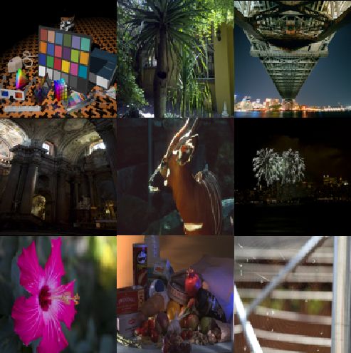
Electronics 2021, 10, 360                                                                                                  2 of 40

                            the data from its compressed form [5–8]. There are many applications for lossless data
                            compression techniques, such as medical imagery, digital radiography, scientific imaging,
                            zip file compression, museums/art galleries, facsimile transmissions of bitonal images,
                            business documents, machine vision, the storage and sending of thermal images taken by
                            nano-satellites, observation of forest fires, etc. [9–13]. In this article, we study the compres-
                            sion standards that are used for lossless image compression. There are many such methods,
                            including run-length coding, Shannon–Fano coding, Lempel–Ziv–Welch (LZW) coding,
                            Huffman coding, arithmetic coding, lossless JPEG, PNG, JPEG 2000, JPEG-LS, JPGE XR,
                            CALIC , AVIF, WebP, FLIF, etc. However, we limit our analysis to lossless JPEG, PNG, JPEG
                            2000, JPEG-LS, JPGE XR , CALIC, AVIF, WebP, and FLIF, since these are the latest and most
                            fully developed methods in this area. Although there are also many types of image, such
                            as binary images, 8-bit and 16-bit grayscale images, 8-bit indexed images, and 8-bit and
                            16-bit red, green, and blue (RGB) images, we only cover 8-bit and 16-bit grayscale and RGB
                            images in this article. A detailed review of run-length, Shannon–Fano, LZW, Huffman, and
                            arithmetic coding was carried out in [3]. Four parameters are used to evaluate a lossless
                            image compression algorithm: the compression ratio (CR), bits per pixel (bpp), encoding
                            time (ET), and decoding time (DT), and bpp is the simply the inverse of the CR; therefore,
                            we only consider the CR, ET, and DT when evaluating these methods. Most studies in
                            this research area use only the CR to evaluate the effectiveness of an algorithm [14–17].
                            Although there are many applications for which higher CRs are important, others may
                            require higher encoding or decoding speeds. Other applications may require high CR and
                            low ET, low ET and DT, or high CR and decoding speed. In addition, there are also many
                            applications where all three of these parameters are equally important. In view of this, we
                            present an extensive analysis from each perspective, and then examine the strength of each
                            algorithm for each kind of image. We compare the performance of these methods based
                            on public open datasets. More specifically, the main aim of this research is to address the
                            following research issues:
                            RI1: How good is each algorithm in terms of the CR for 8-bit and 16-bit greyscale and RGB
                                 images?
                            RI2: How good is each algorithm in terms of the ET for 8-bit and 16-bit greyscale and RGB
                                 images?
                            RI3: How good is each algorithm in terms of the DT for 8-bit and 16-bit greyscale and RGB
                                 images?
                            RI4: How good is each algorithm in terms of the CR and ET for 8-bit and 16-bit greyscale
                                 and RGB images?
                            RI5: How good is each algorithm in terms of the CR and DT for 8-bit and 16-bit greyscale
                                 and RGB images?
                            RI6: How good is each algorithm in terms of the ET and DT for 8-bit and 16-bit greyscale
                                 and RGB images?
                            RI7: How good is each algorithm when all parameters are equally important for 8-bit and
                                 16-bit greyscale and RGB images?
                            RI8: Which algorithms should be used for each kind of image?
                                  The remainder of this article is structured, as follows. In Section 2, we give a brief introduc-
                            tion to the four types of image. In Section 3, we briefly discuss why compression is important,
                            how images are compressed, the kind of changes that occur in data during compression, and
                            the types of data that are targeted during compression. The measurement parameters that are
                            used to evaluate a lossless image compression algorithm are discussed in Section 4. In Section 5,
                            we give a brief introduction to the advanced lossless image compression algorithms. Based
                            on the usual parameters that were used to evaluate a lossless image compression technique
                            and our developed technique, a detailed analysis of the experimental outcomes obtained using
                            these algorithms is provided in Section 6. We conclude the paper in Section 7.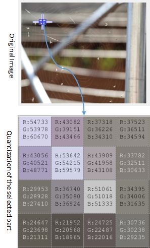
Electronics 2021, 10, 360                                                                                              3 of 40

                               2. Background
                                    A visual representation of an object is called an image, and a digital image can be
                               defined as a two-dimensional matrix of discrete values. When the colour at each position
                               in an image is represented as a single tone, this is referred to as a continuous tone image.
                               The quantised values of a continuous tone image at discrete locations are called the grey
                               levels or the intensity [18], and the pixel brightness of a digital image is indicated by its
                               corresponding grey level. Figure 1 shows the steps that are used to transform a continuous
                               tone image to its digital form.

                            Figure 1. Steps used to convert a continuous tone image to a digital one.

                                    The bit depth indicates the number of bits used to represent a pixel, where a higher bit
                               depth represents more colours, thus increasing the file size of an image [19]. A greyscale
                               image is a matrix of A × B pixels, and 8-bit and 16-bit greyscale images contain 28 = 256
                               and 216 = 65,536 different colours, respectively, where the ranges of colour values are from
                               0–255 and 0–65,535. Figures 2 and 3 show examples of 8-bit and 16-bit greyscale images,
                               respectively.
                                    A particular way of representing colours is called the colour space, and a colour
                               image is a linear combination of these colours. There are many colour spaces, but the most
                               popular are RGB, hue, saturation, value (HSV), and cyan, magenta, yellow, and key (black)
                               (CMYK). RGB contains the three primary colours of red, green, and blue, and it is used by
                               computer monitors. HSV and CMYK are often used by artists and in the printing industry,
                               respectively [18]. A colour image carries three colours per pixel; for example, because an
                               RGB image uses red, green, and blue, each pixel of an 8-bit RGB image has a precision of
                               24 bits, and the image can represent 224 = 16,777,216 different shades. For a 16-bit RGB
                               image, each pixel has a precision of 48 bits, allowing for 248 = 281,474,976,710,656 different
                               shades. Figures 4 and 5 show typical examples of 8-bit and 16-bit RGB images, respectively.
                               The ranges of colour values for 8-bit and 16-bit images are 0–255 and 0–65,535, respectively.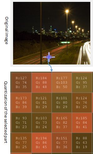
Electronics 2021, 10, 360                                         4 of 40

                            Figure 2. An 8-bit greyscale image.

                            Figure 3. A 16-bit greyscale image.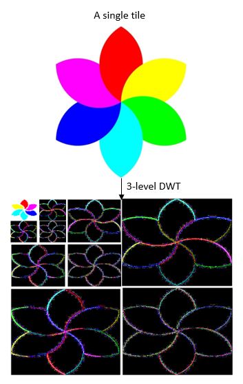
Electronics 2021, 10, 360                                                                                       5 of 40

                            Figure 4. An 8-bit red, green, and blue (RGB) image.

                                 For an uncompressed image (X), the memory that is required to store the image is
                            calculated using Equation (1), where the dimensions of the image are A×B, the bit depth is
                            N, and required storage is S.
                                                                S = ABN2−13 KB                                     (1)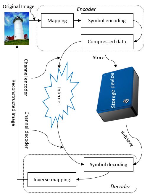
Electronics 2021, 10, 360                                                                                            6 of 40

                            Figure 5. A 16-bit RGB image.

                            3. Data Compression
                                  Data compression is a significant issue and a subject of intense research in the field of
                            multimedia processing. We give a real example below to allow for a better understanding
                            of the importance of data compression. Nowadays, digital cinema and high-definition
                            television (HDTV) use a 4K system, with approximately 4096 × 2160 pixels per frame [20].
                            However, the newly developed Super Hi-Vision (SHV) format uses 7680 × 4320 pixels per
                            frame, with a frame rate of 60 frames per second [21]. Suppose that we have a three-hour
                            colour video file that is based on SHV video technology, where each pixel has a precision
                            of 48 bits. The size of the video file will then be (7680 × 4320 × 48 × 60 × 3 × 60 × 60)
                            bits, or approximately 120,135.498 GB. According to the report in [22], 500 GB to 1 TB is
                            appropriate for storing movies for non-professional users. Seagate, which is an American
Electronics 2021, 10, 360 7 of 40
data storage company, has published quarterly statistics since 2015 on the average capacity
of Seagate hard disk drives (HDDs) worldwide. In the third quarter of 2020, this capacity
was 4.1 TB [23]. Can we imagine what would have happened? We could not even store a
three-hour color SHV video file on our local computer. Compression is another important
issue for data transmission over the internet. Although there are many forms of media that
can be used for transmission, fibre optic cables have the highest transmission speed [24],
and can transfer up to 10 Gbps [25]. If this video file is transferred at the highest speed
available over fibre optic media without compression, approximately 26.697 h would be
required, without considering latency. Latency is the amount of time that is required
to transfer data from the original source to the destination [26]. In view of the above
problems, current technology is entirely inadequate, and data compression is the only
effective solution.
An image is a combination of information and redundant data. How much information
an image contains is one of the most important issues in image compression. If an image
contains a number of unique symbols SL, and P(k) is the probability of the kth symbol,
the average information content (AIC) that an image may contain, which is also known
as entropy, is calculated using Equation (2). Image compression is achieved through a
reduction in redundant data.
SL
AIC = − ∑ log( P(k)) P(k) (2)
k =1
Suppose that two datasets A and B point to the same image or information. Equa-
tion (3) can then be used in order to define the relative data redundancy (Rdr ) of set A,
where the CR is calculated using Equation (4).
1
Rdr = 1 − (3)
CR
A
CR = (4)
B
Three results can be deduced from Equations (3) and (4).
1. When A = B, CR = 1, Rdr = 0, there is no redundancy, and, hence, no compression.
2. When B
A, CR → infinite, Rdr → 1, dataset A contains the highest redundancy
and the greatest compression is achieved.
3. When B
A, CR → 0, Rdr → −in f inite, dataset B contains large memory than the
original (A).
In digital image compression, there are three types of data redundancy: coding, inter-
pixel, and psycho-visual redundancy [27,28]. Suppose that we have the image that is shown
in Figure 6 with the corresponding grey levels.
The 10 × 10 image shown in Figure 6 contains nine different values (S) (118, 119,
120, 139, 140, 141, 169, 170, 171), and for a fixed code length, each value can be coded
as an 8-bit code-word, since the maximum value (171) requires a minimum of 8 bits to
code. Consequently, 800 bits are required to store the image. In contrast, a variable code
length is based on probability, where codes of shorter length are assigned to values with
higher probability. The probability of the kth values is calculated while using Equation (5),
where N is the total number of values in an image. If Lk represents the length of the
code-word for the values Sk , then the length of the average code-word can be calculated
using Equation (6), where SL is the total number of different values. Table 1 shows the
variable length coding for the image shown in Figure 6.
Sk
P(k) = (5)
NElectronics 2021, 10, 360 8 of 40
SL
L avg = ∑ Lk P(k ) (6)
k =1
Figure 6. An image with the corresponding pixel values.
Table 1. Variable length coding for the image in Figure 6.
Symbol Probability Code-Word Code-Word Lk Pk
(S) (P(k)) Length (Lk )
118 0.12 100 3 0.36
119 0.16 001 3 0.48
120 0.12 011 3 0.36
139 0.01 1111 4 0.04
140 0.17 000 3 0.51
141 0.12 010 3 0.36
169 0.11 101 3 0.33
170 0.09 1110 4 0.36
171 0.1 110 3 0.3
L avg = 3.1 bits
From Table 1, we obtain approximate values of CR = 2.581 and Rdr = 0.613, and the
compressed image takes 300 bits rather than 800 bits. These results show that the original
image contains redundant code, and that the variable length coding has removed this
redundancy [29,30].
Interpixel redundancy can be classified as spatial, spectral, and temporal redundancy.
In spatial redundancy, there are correlations between neighbouring pixel values, whereas,
in spectral redundancy, there are correlations between different spectral bands. In temporal
redundancy, there are correlations between the adjacent frames of a video. Interpixel redun-
dancy can be removed using run-length coding, the differences between adjacent pixels,
predicting a pixel using various methods, thresholding, or various types of transformation
techniques, such as discrete Fourier transform (DFT) [31].
To remove interpixel redundancy from the image presented in Figure 7 using run-
length coding, we code the image, as follows: (120,1) (119,1) (118,8) (120,1) (119,8) (118,1)
(120,9) (119,1) (120,1) (119,6) (118,3) (141,1) (140,8) (139,1) (141,6) (140,4) (141,5) (140,5)
(171,1) (170,2) (169,7) (171,2) (170,4) (169,4) (171,7) (170,3), requiring 312 bits. Twelve bitsElectronics 2021, 10, 360 9 of 40
are required to code each pair, and an 8-bit code word is used for the grey level, since the
maximum gray level is 171. A 4-bit code word is used for the length of the grey level, since
the maximum value for the length of the gray level is nine.
The main purpose of using prediction or transformation techniques can be described,
as follows. To create a narrow histogram, a prediction or various other types of transforma-
tion techniques can be applied to provide a small value for the entropy. For example, we
apply the very simple predictor that is given below to the image shown in Figure 6, where
0
A represents the predicted pixels. Figure 7a shows the histogram of the original image,
and Figure 7b shows the histogram obtained after applying the predictor that is shown in
Equation (7).
0
A ( p, q) = A( p, q − 1) − A( p, q) (7)
Figure 7. A comparison of histograms before and after application of a predictor.
Figure 7 shows that the histogram of the original image contains nine different values,
of which eight have approximately the same frequency, and the highest frequency is 17.
After applying the predictor, the histogram only contains five values, of which only two
(0 and 1) contain 90% of the data, thus giving a better compression ratio. The interpixel
redundancy of an image can be removed using one or more techniques in combination. For
example, after applying the predictor to the original image presented in Figure 6, we can
apply both run-length and Huffman coding, with the result that only 189 bits are required
to store the image rather than 800 bits.
The construction of an image compression technique is highly application-specific.
Figure 8 shows a general block diagram of lossless image compression and decompression.
The mapping that is shown in Figure 8 is used to convert an image into a non-visual
form to decrease the interpixel redundancy. Run-length coding, various transformation
techniques, and prediction techniques are typically applied at this stage. At the symbol
encoding stage, Huffman, arithmetic, and other coding methods are often used to reduce
the coding redundancy. The image data are highly correlated, and the mapping process is
a very important way of decorrelating the data and eliminating redundant data. A better
mapping process can eliminate more redundant data and give better compression. The
first and most important problem in image compression is to develop or choose an optimal
mapping process, while the second is to choose an optimal entropy coding techniqueElectronics 2021, 10, 360 10 of 40
to reduce coding redundancy [32]. In channel encoding, Hamming coding is applied to
increase noise immunity, whereas, in decoding, the inverse procedures are applied to
provide a lossless decompressed image. Quantisation, which is an irreversible process,
removes irrelevant information by reducing the number of grey levels, and it is applied
between the mapping and symbol encoding stages in lossy image compression [33–38].
Figure 8. Basic block diagram of lossless image compression.
4. Measurement Standards
Measurement standards offer ways of determining the efficiency of an algorithm. The
four measurement standards (compression ratios, encoding time, decoding time, and bits
per pixel) are used to evaluate a lossless image compression algorithm.
The CR is the ratio between the size of an uncompressed image and its compressed
version. Entropy is generally estimated as the average code length of a pixel in an image;
however, in reality, this estimate is overoptimistic due to statistical interdependencies
among pixels. For example, Table 1 shows that the CR is 2.581, but the estimated entropy
for the same data is 3.02. Hence, the entropy-based compression ratio is 2.649. Equation (4)
is used to calculate the CR to solve this issue. The bpp [39] is the number of bits used to
represent a pixel, i.e. the inverse of the CR, as shown in Equation (8). The ET and DT are
the times that are required by an algorithm to encode and decode an image, respectively.
B
bpp = (8)
A
5. State-of-the-Art Lossless Image Compression Techniques
The algorithms used for lossless image compression can be classified into four cate-
gories: entropy coding (Huffman and arithmetic coding), predictive coding (lossless JPEG,Electronics 2021, 10, 360 11 of 40
JPEG-LS, PNG, CALIC), transform coding (JPEG 2000, JPEG XR), and dictionary-based
coding (LZW). All of the predictive and transform-based image compression techniques
use an entropy coding strategy or Golomb coding as part of their compression procedure.
5.1. Lossless JPEG and JPEG-LS
The Joint Photographic Experts Group (JPEG) format is a DCT-based lossy image
compression technique, whereas lossless JPEG is predictive. Lossless JPEG uses the 2D
differential pulse code modulation (DPCM) scheme [40], and it predicts a value (P) for the
current pixel (P) that is based on up to three neighbouring pixels (A, B, D). Table 2 shows
the causal template used to predict a value. If two pixels (B, D) from Table 2 are considered
in this prediction, then the predicted value (P) and prediction error (PE) are calculated
while using Equations (9) and (10), respectively.
Table 2. Causal template.
E F G Past pixels
H A B C Current pixel
K D P Future pixels
D+B
P= (9)
2
PE = P − P (10)
Consequently, the prediction errors remain close to zero, and very large positive or
negative errors are not commonly seen. Therefore, the error distribution looks almost like
a Gaussian normal distribution. Finally, Huffman or arithmetic coding is used to code
the prediction errors. Table 3 shows the predictor that is used in the lossless JPEG format,
based on three neighbouring pixels (A, B, D). In lossy image compression, three types of
degradation typically occur and should be taken into account when designing a DPCM
quantiser: granularity, slope overload, and edge-busyness [41]. DPCM is most sensitive to
channel noise.
Table 3. Predictor for Lossless Joint Photographic Experts Group (JPEG).
Mode Predictor
0 No prediction
1 D
2 B
3 A
4 D+B−A
5 D + (B − A)/2
6 B + (D − A)/2
7 (D + B)/2
A real image usually has a nonlinear structure, and the DPCM uses a linear predictor,
This is why problems can occur. This gave rise to the need to develop a perfect nonlinear
predictor. The median edge detector (MED) is one of the most widely used nonlinear
predictors, which is used by JPEG-LS to address these drawbacks.
JPEG-LS was designed based on LOCO-I (Low Complexity Lossless Compression
for Images) [42,43], and a standard was eventually introduced in 1999 after a great deal
of development [44–47]. JPEG-LS improves the context modelling and encoding stages
by applying the same concept as lossless JPEG. Although the discovery of arithmeticElectronics 2021, 10, 360 12 of 40
codes [48,49] conceptually separates the stages, the separation process becomes less clean
under low-complexity coding constraints, due to the use of an arithmetic coder [50]. In
context modelling, the number of parameters is an important issue, and it must be reduced
to avoid context dilution. The number of parameters depends entirely on the number of
context. A two-sided geometric distribution (TSGD) model is assumed for the prediction
residuals to reduce the number of parameters. The selection of a TSGD model is a significant
issue in a low-complexity framework, since a better model only needs very simple coding.
Merhav et al. [51] showed that adaptive symbols can be used in a scheme, such as Golomb
coding, rather than more complex arithmetic coding, since the structure of Golomb codes
provides a simple calculation without requiring the storage of code tables. Hence, JPEG-LS
uses Golomb codes at this stage. Lossless JPEG cannot provide an optimal CR, because it
cannot de-correlate by first order entropy of their prediction residuals. In contrast, JPEG-
LS can achieve good decorrelation and provide better compression performance [42,43].
Figure 9 shows a general block diagram for JPEG-LS.
Figure 9. Block diagram for the JPEG-LS encoder [43].
The prediction or decorrelation process of JPEG-LS is completely different from that
in lossless JPEG. The LOCO-I or MED predictor used by JPEG-LS [52] predicts a value ( P)
according to Equation (11), as shown in Table 2.
min( D, B), if C ≥ max ( D, B)
P = max ( D, B), if C ≤ min( D, B) (11)
D + B − A, otherwise.
5.2. Portable Network Graphics
Portable Network Graphics (PNG) [53–55], a lossless still image compression scheme,
is an improved and patent-free replacement of the Graphics Interchange Format (GIF). It is
also a technique that uses prediction and entropy coding. The deflate algorithm, which is a
combination of LZ77 and Huffman coding, is used as the entropy coding technique. PNG
uses five types of filter for prediction [56], as shown in Table 4 (based on Table 2).Electronics 2021, 10, 360 13 of 40
Table 4. Predictor for Portable Network Graphics (PNG)-based image compression.
Type Byte Filter Name Prediction
0 None Zero
1 Sub D
2 Up B
3 Average The rounded mean of D and B
4 Paeth [56] One of D, B, or A (whichever
is closest to P = D + B − A)
5.3. Context-Based, Adaptive, Lossless Image Codec
Context-based, adaptive, lossless image codec (CALIC) is a lossless image compression
technique that uses a more complex predictor (gradient-adjusted predictor, GAP) than
lossless JPEG, PNG, and JPEG-LS. GAP provides better modelling than MED by classifying
the edges of an image as either strong, normal, or weak. Although CALIC provides more
compression than JPEG-LS and better modelling, it is computationally expensive. Wu [57]
used the local horizontal (Gh).and vertical (Gv) image gradients (Equations (12) and (13)) to
predict a value ( P) (Equation (14)) for the current pixel (P) using Equation (15), as shown in
Table 2. At the coding stage, CALIC uses either Huffman coding or arithmetic coding; the
latter provides more compression, but it takes more time for encoding and decoding, since
arithmetic coding is more complex. The encoding and decoding methods in CALIC follow
a raster scan order, with a single pass of an image. There are two modes of operation, binary
and continuous tone. If the current locality of an original image has a maximum of two
distinct intensity values, binary mode is used; otherwise, continuous tone mode is used.
The continuous tone approach has four components: prediction, context selection and
quantisation, context modelling of prediction errors, and entropy coding of the prediction
errors. The mode is selected automatically, and no additional information is required [58].
Gh = | D − K | + | B − A| + |C − B| (12)
Gv = | D − A| + | B − F | + |C − G | (13)
D,
if( Gv − Gh > 80); Sharp horizontal edge
M + P
if( Gv − Gh
2 ,
> 32); Horizontal edge
3× M+ P , if( Gv − Gh
> 8); Weak horizontal edge
P= 4 (14)
B, if( Gv − Gh < −80); Sharp vertical edge
M + B
2 , if( Gv − Gh < −32); Vertical edge
3× M+ B , if( Gv − Gh
< −8); Weak vertical edge
4
D+B C−A
M= + (15)
2 4
5.4. JPEG 2000
JPEG 2000 is an extension complement of the JPEG standard [40], and it is a wavelet-
based still image compression technique [59–62] with certain new functionalities. It pro-
vides better compression than JPEG [60]. The development of JPEG 2000 began in 1997,
and became an international standard [59] in 2000. It can be used in lossless or lossy com-
pression within a single architecture. Most image or video compression standards divide
an image or a video frame into square blocks, to be processed independently. For example,
JPEG uses the Discrete Cosine Transform (DCT) in order to split an image into a set of
8 × 8 square blocks for transformation. As a result of this processing, extraneous blocking
artefacts arise during the quantisation of the DCT coefficients at high CR [7], producing
visually perceptible faults in the image [61–64]. In contrast, JPEG 2000 transforms an imageElectronics 2021, 10, 360 14 of 40
as a whole while using a discrete wavelet transformation (DWT), and this addresses the
issue. One of the most significant advantages of using JPEG 2000 is that different parts
of the same image can be saved with different levels of quality if necessary [65]. Another
advantage of using DWT is that it transforms an image into a set of wavelets, which are
easier to store than pixel blocks [66–68]. JPEG 2000 is also scalable, which means that a
code stream can be truncated at any point. In this case, the image can be constructed, but
the resolution may be poor if many bits are omitted. JPEG 2000 has two major limitations:
it produces ringing artifacts near the edges of an image, and is computationally more
expensive [69,70]. Figure 10 shows a general block diagram for the JPEG 2000 encoding
technique.
Figure 10. (a) JPEG 2000 encoder; (b) dataflow [68].
Initially, an image is transformed into the YUV colour space, rather than YCbCr,
for lossless JPGE2000 compression, since YCbCr is irreversible and YUV is completely
reversible. The transformed image is then split into a set of tiles. Although the tiles may be
of any size, all of the tiles in an image are the same size. The main advantage of dividing an
image into tiles is that the decoder requires very little memory for image decoding. In this
tiling process, the image quality can be decreased for low PSNR, and the same blocking
artifacts, like JPEG, can arise when more tiles are created. The LeGall-Tabatabai (LGT) 5/3
wavelet transform is then used to decompose each tile for lossless coding [71,72], while the
CDF 9/7 wavelet transform is used for lossy compression [72].
Quantisation is carried out in lossy compression, but not in lossless compression.
The outcome of the transformation process is the sub-band collection and the sub-bands
are further split into code blocks, which are then coded while using the embedded block
coding with optimal truncation (EBCOT) process, in which the most significant bits areElectronics 2021, 10, 360 15 of 40
coded first. All of the bit planes of the code blocks are perfectly stored and coded, and a
context-driven binary arithmetic coder is applied as an entropy coder independently to
each code block. Some bit planes are dropped in lossy compression. While maintaining the
same quality, JPEG 2000 provides about 20% more compression than JPEG and it works
better for larger images.
After the DWT transformation of each tile, we obtain four parts: the top left image
with lower resolution, the top right image with higher vertical resolution, the bottom left
image with lower vertical resolution, and the bottom right image with higher resolution in
both directions. This decomposition process is known as dyadic [60], and it is illustrated in
Figure 11 based on a real image, where the entire image is considered as a single tile.
Figure 11. Dyadic decomposition of a single tile.
5.5. JPEG XR (JPEG Extended Range)
Like JPEG, JPEG Extended Range (JPEG XR) is a still image compression technique
that was developed based on HD photo technology [73,74]. The main aim of the design
of JPEG XR was to achieve better compression performance with limited computational
resources [75], since many applications require a high number of colours. JPEG XR can
represent 2.8 ×10¹⁴ colours, as compared to only 16,777,216 for JPEG. While JPEG-LS, CALIC,
and JPEG 2000 use MED, GAP, and DWT, respectively, for compression, JPEG XR uses a
lifting-based reversible hierarchical lapped biorthogonal transform (LBT). The two mainElectronics 2021, 10, 360 16 of 40
advantages of this transformation are that encoding and decoding both require relatively
few calculations, and they are completely reversible. Two operations are carried out in this
transformation: a photo core transform (PCT), which employs a lifting scheme, and a photo
overlap transform (POT) [76]. Similar to DCT, PCT is a 4 × 4 wavelet-like multi-resolution
hierarchical transformation within a 16 × 16 macroblock. This transformation improves the
image compression performance [76]. POT is performed before PCT to reduce blocking
artifacts at low bitrates. Another advantage of using POT is that it reduces the ET and DT at
high bitrates [77]. At the quantisation stage, a flexible coefficient quantisation approach that
is based on the human visual system is used that is controlled by a quantisation factor (QF),
where QF varies, depending on the colour channels, frequency bands, and spatial regions of the
image. It should be noted that quantisation is only done for lossy compression. An inter-block
coefficient prediction technique is also implemented to remove inter-block redundancy [74].
Finally, JPEG XR uses adaptive Huffman coding as an entropy coding technique. JPEG XR
also allows for image tiling in the same way as JPEG 2000, which means that the decoding of
each block can be done independently. JPEG XR permits multiple colour conversions, and
uses the YCbCr colour space for images with 8 bits per sample and the YCoCg color space for
RGB images. It also supports the CMYK colour model [73]. Figures 12 and 13 show general
block diagrams for JPEG XR encoding and decoding, respectively.
Figure 12. JPEG XR encoder [78].
Figure 13. JPEG XR decoder [74].Electronics 2021, 10, 360 17 of 40
5.6. AV1 Image File Format (AVIF), WebP and Free Lossless Image Format (FLIF)
In 2010, Google introduced WebP based on VP8 [79]. It is now one of the most success-
ful image formats and it supports both lossless and lossy compression. WebP predicts each
block based on three neighbor blocks, and the blocks are predicted in four modes: horizon-
tal, vertical, DC, and TrueMotion [80,81]. Though WebP provides better compression than
JPEG and PNG, only some browsers support WebP. Another disadvantage is that lossless
WebP does not support progressive decoding [82]. A clear explanation of the encoding
procedure of WebP has been given in [83].
AOMedia Video 1 (AV1), which was developed in 2015 for video transmission, is a
royalty-free video coding format [84], and AV1 Image File Format (AVIF) is derived from
AV1 and it uses the same technique for image compression. It supports both lossless and
lossy compression. AV1 uses a block-based frequency transform and incorporates some
new features that are based on Google’s VP9 [85]. As a result, the AV1’s encoder gets
more alternatives to allow for better adaptation to various kinds of input and outperforms
H.264 [86]. The detailed coding procedure of AV1 is given in [87,88]. AVIF and HEIC
provide almost similar compression. HEIC is patent-encumbered H.265 format and illegal
to use without obtaining patent licenses. On the other hand, AVIF is free to use. There are
two biggest problems in AVIF. It is very slow for encoding and decoding an image, and
it does not support progressive rendering. AVIF provides many advantages over WebP.
For example, it provides a smaller sized image and a more quality image, and it supports
multi-channel [89]. A detailed encoding procedure of AV1 is shown in [90].
Free Lossless Image Format (FLIF) is one of the best lossless image formats and it
provides better performance than the state-of-the-art techniques in terms of compression
ratio. Many image compression techniques (e.g., PNG) support progressive decoding that
can show an image without downloading the whole image. In this stage, FLIF is better, as it
uses progressive interlacing, which is an improved version of the progressive decoding of
PNG. FLIF is developed based on MANIAC (Meta-Adaptive Near-zero Integer Arithmetic
Coding), a variant of CABAC (context-adaptive binary arithmetic coding. The detailed
coding explanation of FLIF is given in [91,92]. One of the main advantages of FLIF is that
it is responsive by design. As a result, users can use it, as per their needs. FLIF provides
excellent performances on any kind of image [93]. In [91], Jon et al. show that JPEG and
PNG work well on photographs and drawings images, respectively, and there is no single
algorithm that works well on all types of images. However, they finally conclude that only
FLIF works better on any kinds of image. FLIF has many limitations, such as no browser
still supports FLIF [94], and it takes more time for encoding and decoding an image.
6. Experimental Results and Analysis
The dependence of many applications on multimedia computing is growing rapidly,
due to an increase in the use of digital imagery. As a result, the transmission, storage, and
effective use of images are becoming important issues. Raw image transmission is very
slow, and gives rise to huge storage costs. Digital image compression is a way of converting
an image into a format that can be transferred quickly and stored in a comparatively small
space. In this paper, we provide a detailed analysis of the state-of-the-art lossless still image
compression techniques. As we have seen, most previous survey papers on lossless image
compression focus on the CR [3,4,16,78,95–98]. Although this is an important measurement
criterion, the ET and DT are two further important factors for lossless image compression.
The key feature of this paper is that we not only carry out a comparison based on CR, but
also explore the effectiveness of each algorithm in terms of compressing an image based on
several metrics. We use four types of images: 8-bit and 16-bit greyscale and RGB images.
We applied state-of-the-art techniques to a total of nine uncompressed images of each type,
taken from a database entitled “New Test Images—Image Compression Benchmark” [99].Electronics 2021, 10, 360 18 of 40
6.1. Analysis Based on Usual Parameters
In this section, we have analysed based on every single parameter. Figures 14–16
show the 8-bit greyscale images and their respective ETs and DTs, and Table 5 shows the
CRs of the images. Table 5 shows that FLIF gives the highest CR for the artificial.pgm,
big_tree.pgm, bridge.pgm, cathedral.pgm, fireworks.pgm, and spider_web.pgm 8-bit
greyscale images. For the rest of the images, AVIF provides the highest CR. JPEG XR
gives the lowest CRs (3.196, 3.054, and 2.932) for three images (artificial, fireworks and
flower_foveon, respectively), while for the rest of the images, lossless JPEG gives the lowest
CR. In terms of the ET, Figure 15 shows that JPEG-LS gives the shortest times (0.046 and
0.115 s) for two images (artificial and fireworks) and JPEG XR gives the shortest times
for the remainder of the images. FLIF takes the longest times ( 3.28, 15.52, 6.18, 2.91, 6.19,
2.73, 3.27 and 4.32 s, respectively) for all the images, except flower_foveon.pgm. For this
image, AVIF takes the longest time (1.54 s). Figure 16 shows that, at the decoding stage,
CALIC takes the longest times (0.542, 0.89, and 0.898 s) for three images (fireworks.pgm,
hdr.pgm, and spider_web.pgm, respectively), and WebP takes the longest times (3.26 and
2.33 s) for two images (big_tree.pgm and bridge.pgm, respectively), while FLIF takes the
longest times for the rest of the images. On the other hand, PNG takes the shortest times,
respectively, for all of the images.
Table 5. Comparison of compression ratios for 8-bit greyscale images.
Image Name JPEG Lossless JPEG
JPGE-LS PNG CALIC AVIF WebP FLIF
(Dimensions) 2000 JPEG XR
artificial.pgm 10.030 6.720 4.884 8.678 3.196 10.898 4.145 10.370 13.260
(2048 × 3072)
big_tree.pgm 2.144 2.106 1.806 1.973 2.011 2.159 2.175 2.145 2.263
(4550 × 6088)
bridge.pgm 1.929 1.910 1.644 1.811 1.846 1.929 1.973 1.943 1.979
(4049 × 2749)
cathedral.pgm 2.241 2.160 1.813 2.015 2.038 2.254 2.222 2.217 2.365
(3008 × 2000)
deer.pgm 1.717 1.748 1.583 1.713 1.685 1.727 1.872 1.794 1.775
(2641 × 4043)
fireworks.pgm 5.460 4.853 3.355 4.095 3.054 5.516 4.486 4.858 5.794
(2352 × 3136)
flower_foveon.pgm 3.925 3.650 2.970 3.054 2.932 3.935 4.115 3.749 3.975
(1512 × 2268)
hdr.pgm 3.678 3.421 2.795 2.857 2.847 3.718 3.825 3.456 3.77
(2048 × 3072)
spider_web.pgm 4.531 4.202 3.145 3.366 3.167 4.824 4.682 4.133 4.876
(2848 × 4256)Electronics 2021, 10, 360 19 of 40
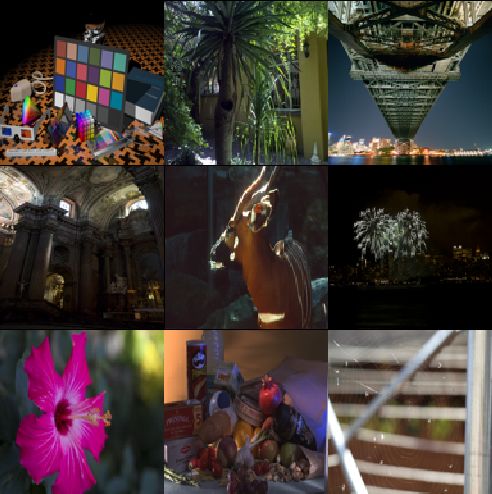
Figure 14. Examples of 8-bit greyscale images.
Figure 15. Encoding times for 8-bit greyscale images.
Figure 17 shows examples of 8-bit RGB images. Table 6 and Figures 18 and 19 show
the values of CR, ET, and DT for each of the images. From Table 6, it can be seen that FLIF
gives the highest CRs (18.446 and 5.742) for two images (artificial.PPM and fireworks.PPM,
respectively), and AVIF gives the highest CRs for the rest of the images. JPEG XR gives the
lowest CRs (4.316 and 3.121) for two images (artificial and fireworks, respectively) and, for
the remaining seven images, lossless JPEG gives the lowest CRs. Figure 18 shows that FLIF
requires the longest ETs for all the images. JPEG XR gives the shortest ET for all images, exceptElectronics 2021, 10, 360 20 of 40
artificial.pgm, for which JPEG-LS gives the shortest ET (0.16 s). For decoding, CALIC takes the
longest time for all images, except for bridge, cathedral, and deer, as shown in Figure 19, and
FLIF takes the longest times (4.75, 2.379, and 5.75 s, respectively) for these images. Figure 19
also shows that JPEG XR takes the shortest time (0.157 s) to decode artificial.ppm, and PNG
takes the shortest for the rest of the images.
Figure 16. Decoding times for 8-bit greyscale images.
Figure 17. Examples of 8-bit RGB images.Electronics 2021, 10, 360 21 of 40
Table 6. Comparison of compression ratios for 8-bit RGB images.
Image Name JPEG Lossless JPEG
JPGE-LS PNG CALIC AVIF WebP FLIF
(Dimensions) 2000 JPEG XR
artificial.pgm 10.333 8.183 4.924 10.866 4.316 10.41 6.881 17.383 18.446
(2048 × 3072)
big_tree.pgm 1.856 1.823 1.585 1.721 1.719 1.886 2.254 1.835 1.922
(4550 × 6088)
bridge.pgm 1.767 1.765 1.553 1.686 1.735 1.784 2.21 1.748 1.866
(4049 × 2749)
cathedral.pgm 2.120 2.135 1.734 1.922 2.015 2.126 2.697 2.162 2.406
(3008 × 2000)
deer.pgm 1.532 1.504 1.407 1.507 1.480 1.537 1.915 1.567 1.588
(2641 × 4043)
fireworks.pgm 5.262 4.496 3.279 3.762 3.121 5.279 5.432 4.624 5.742
(2352 × 3136)
flower_foveon.pgm 3.938 3.746 2.806 3.149 3.060 3.927 5.611 4.158 4.744
(1512 × 2268)
hdr.pgm 3.255 3.161 2.561 2.653 2.716 3.269 4.614 3.213 3.406
(2048 × 3072)
spider_web.pgm 4.411 4.209 3.029 3.365 3.234 4.555 6.017 4.317 4.895
(2848 × 4256)
Figure 18. Comparison of encoding times for 8-bit RGB images.Electronics 2021, 10, 360 22 of 40
Figure 19. Comparison of decoding times for 8-bit RGB images.
Figures 20–22 and Table 7 show the 16-bit greyscale images and their respective ETs,
DT, and CRs. From Table 7, it can be seen that FLIF gives the highest CRs for all the images
except deer.pgm, flower_foveon.pgm, and hdr.pgm. For these images, AVIF provides the
highest CRs (3.742, 8.273, and 7.779, respectively). Lossless JPEG gives the lowest CR (2.791)
for artificial.pgm, and PNG gives the lowest for the rest of the images. Figure 21 shows that
FLIF gives the highest ETs for all the images, except big_tree.pgm. For this image, JPEG 2000
takes the highest (4.579 s). JPEG-LS gives the lowest ETs (0.186, 0.238, 0.257, and 0.406 s) for
four images (artificial, cathedral, fireworks, and spider_web, respectively) and JPEG XR gives
the lowest for the rest of the images. In terms of decoding, CALIC and lossless JPEG give the
highest DTs (0.613 and 0.503 s) for artificial.pgm and flower_foveon.pgm, respectively, and
JPEG 2000 gives the highest DTs (1.078, 0.978, and 1.736 s) for three images (fireworks, hdr,
and spider_web, respectively). For the rest of the images, FLIF takes the highest DTs. On the
other hand, PNG gives the lowest DTs for all of the images shown in Figure 22.Electronics 2021, 10, 360 23 of 40
Figure 20. Examples of 16-bit greyscale images.
Figure 21. Comparison of encoding times for 16-bit greyscale images.Electronics 2021, 10, 360 24 of 40
Figure 22. Comparison of decoding times for 16-bit greyscale images.
Table 7. Comparison of compression ratios for 16-bit greyscale images.
Image Name JPEG Lossless JPEG
JPGE-LS PNG CALIC AVIF WebP FLIF
(Dimensions) 2000 JPEG XR
artificial.pgm 4.073 4.007 2.791 4.381 6.393 4.174 8.282 20.846 26.677
(2048 × 3072)
big_tree.pgm 1.355 1.325 1.287 1.181 4.028 1.324 4.35 4.229 4.537
(4550 × 6088)
bridge.pgm 1.309 1.279 1.244 1.147 3.696 1.373 3.944 3.843 3.971
(4049 × 2749)
cathedral.pgm 1.373 1.337 1.293 1.191 4.084 1.342 4.450 4.398 4.749
(3008 × 2000)
deer.pgm 1.252 1.241 1.225 1.132 3.371 1.339 3.742 3.549 3.557
(2641 × 4043)
fireworks.pgm 1.946 1.809 1.740 1.604 6.116 1.955 8.967 9.773 11.647
(2352 × 3136)
flower_foveon.pgm 1.610 1.591 1.523 1.316 5.884 1.663 8.273 7.626 8.029
(1512 × 2268)
hdr.pgm 1.595 1.563 1.491 1.297 5.755 1.569 7.779 7.040 7.754
(2048 × 3072)
spider_web.pgm 1.736 1.771 1.554 1.367 6.386 1.742 9.658 8.442 10.196
(2848 × 4256)
Figure 23, Table 8, and Figures 24 and 25 show the 16-bit RGB images and their CRs,
ETs, and DTs, respectively. From Table 8, it can be seen that FLIF gives the highest CRs
(37.021 and 12.283) for artificial.ppm and fireworks.ppm, respectively, and AVIF for theElectronics 2021, 10, 360 25 of 40
rest of the images. Lossless JPEG gives the lowest CRs (2.6952 and 1.6879) for the artificial
and fireworks images, respectively, and PNG gives the lowest for the rest of the images.
In terms of the encoding time, JPEG 2000 gives the highest (14.259, 5.699, and 5.672 s)
for three images (big_tree.pgm, bridge.pgm, and fireworks.pgm, respectively), and FLIF
gives the highest ETs for the rest of the images shown in Figure 24. JPEG XR takes the
lowest ETs for all of the images. Figure 25 shows that CALIC gives the longest DT (2.278 s)
for artificial.ppm, and FLIF gives the longest DTs (2.05, 3.27, and 5.01 s) for three images
(flower_foveon.pgm, hdr.pgm, and spider_web.pgm, respectively), while JPEG 2000 takes
the longest DTs for the rest of the images. PNG gives the shortest DT (0.292, and 0.28s) for
fireworks.pgm and hdr.pgm, respectively, and JPEG XR gives the shortest for the rest of the
images. It should be noted that, although Figures 14 and 20, as well as Figures 17 and 23,
are visually identical, these four figures are completely different in terms of the bit depths
and channels in the images.
Figure 23. Examples of 16-bit RGB images.Electronics 2021, 10, 360 26 of 40
Figure 24. Comparison of encoding times for 16-bit RGB images.
Figure 25. Comparison of decoding times for 16-bit RGB images.Electronics 2021, 10, 360 27 of 40
Table 8. Comparison of compression ratios for 16-bit RGB images.
Image Name JPEG Lossless JPEG
JPGE-LS PNG CALIC AVIF WebP FLIF
(Dimensions) 2000 JPEG XR
artificial.pgm 4.335 4.734 2.695 4.896 8.644 4.404 13.783 36.292 37.021
(2048 × 3072)
big_tree.pgm 1.302 1.261 1.249 1.150 3.441 1.284 4.504 3.614 3.841
(4550 × 6088)
bridge.pgm 1.274 1.243 1.240 1.132 3.470 1.283 4.414 3.445 3.739
(4049 × 2749)
cathedral.pgm 1.379 1.333 1.267 1.218 4.036 1.383 5.397 4.292 4.851
(3008 × 2000)
deer.pgm 1.197 1.173 1.236 1.100 2.961 1.196 3.826 3.096 3.176
(2641 × 4043)
fireworks.pgm 2.378 1.832 1.688 2.053 6.453 2.384 11.318 10.048 12.283
(2352 × 3136)
flower_foveon.pgm 1.724 1.664 1.494 1.371 6.121 1.765 11.217 8.305 9.513
(1512 × 2268)
hdr.pgm 1.535 1.518 1.473 1.275 5.432 1.586 9.219 6.391 6.819
(2048 × 3072)
spider_web.pgm 1.702 1.784 1.531 1.360 6.466 1.718 12.018 8.576 9.787
(2848 × 4256)
Figure 26 shows the average CRs for all four types of image. It can be seen that FLIF
gives the highest (4.451, 9.013, 5.002, and 10.114) CRs for all type of images and it achieves
compression that is 10.99%, 23.19%, 40.1%, 26.2%, 43.14%, 7.73%, 26.38%, and 13.46%
higher for the 8-bit greyscale images, 79.97%, 80.37%, 82.56%, 81.98%, 43.65%, 79.68%,
26.72%, and 14.01% higher for the 16-bit greyscale images, 23.43%, 31.09%, 49.18%, 31.97%,
48.02%, 22.75%, 16.41%, and 8.92% higher for the 8-bit RGB images, and 81.51%, 81.83%,
84.76%, 82.91%, 48.34%, 81.32%, 16.84%, and 7.65% higher for the 16-bit RGB images than
JPEG-LS, JPEG 2000, Lossless JPEG, PNG, JPEG XR, CALIC, AVIF, and WebP, respectively.
If the CR is the main consideration for an application, from Figure 26 we can see that FLIF
is better for all four types of image.
Figure 27 shows the average encoding times. It can be seen that JPEG XR requires
the shortest average ET (0.167, 0.376, 0.455, and 0.417 s) for the 8-bits greyscale, 16-bit
greyscale, 8-bit RGB, and 16-bit RGB images, respectively. In terms of encoding, JPEG XR is
on average 32.39%, 72.03%, 48.77%, 85.17%, 82.49%, 92.08%, 87.44%, and 96.73% faster for
8-bit greyscale images, 20.84%, 75.84%, 19.66%, 69.41%, 55.4%, 79.64%, 75.49%, and 85.35%
faster for 16-bit greyscale images, 41.29%, 78.4%, 58.41%, 84.27%, 84.46%, 82.68%, 81.14%,
and 93.59% faster for 8-bit RGB images, and 61.95%, 91.15%, 72.96%, 88.64% and 83.42%,
84.65%, 83.85%, and 91.63% faster for 16-bit RGB images than JPEG-LS, JPEG 2000, lossless
JPEG, PNG, CALIC, AVIF, WebP, and FLIF, respectively. If the ET is the main consideration
for an application, then we can draw the conclusion that compression using JPEG XR is
best for all types of images.Electronics 2021, 10, 360 28 of 40
Figure 26. Comparison of average compression ratios.
Figure 27. Comparison of average encoding times.
Figure 28 shows the average DT. PNG gives the shortest DT (0.072, 0.161, and 0.223 s)
for the 8-bit greyscale, 16-bit greyscale, and 8-bit RGB images, respectively, while JPEG XRElectronics 2021, 10, 360 29 of 40
gives the shortest (0.398 s) for the 16-bit RGB images. On average, PNG decodes 74.19%,
87.21%, 45.86%, 55.28%, 91.57%, 87.86%, 93.55%, and 93.66% faster for 8-bit greyscale
images, 56.84%, 89.87%, 42.5%, 55.4%, 81.85%, 86%, 85%, and 87% faster for 16-bit greyscale
images, and 75.92%, 88.78%, 56.45%, 52.25%, 91.13%, 88.24%, 87.77%, and 88.95% faster for
8-bit RGB images than JPEG-LS, JPEG 2000, lossless JPEG, JPEG XR, CALIC, AVIF, WebP,
and FLIF, respectively. However, for 16-bit RGB images, JPEG XR is 63.45%, 91.76%, 53.99%,
22.72%, 83.75%, 85.8%, 85.42%, and 87.12% faster than JPEG-LS, JPEG 2000, lossless JPEG,
PNG, CALIC, AVIF, WebP, and FLIF, respectively, for the same case. When DT is the main
consideration for an application during compression, we can conclude from Figure 28 that
PNG is better for 8-bit greyscale, 16-bit greyscale, and 8-bit RGB images, whereas JPEG XR
is better for 16-bit RGB images.
Figure 28. Comparison of average decoding times.
6.2. Analysis Based on Our Developed Technique
Because the performance of a lossless algorithm depends on the CR, ET, and DT,
we develop a technique that is defined in Equations (16)–(19) to calculate the overall
and grand total performance for each algorithm when simultaneously considering all of
these parameters. The overall performance means how good is each method on average
among all methods in terms of each individual evaluation parameter, whereas grand total
performance is a combination of two or more parameters. For each method, the overall
performance (OVP) in terms of CR, ET, and DT is calculated while using Equations (16)–(18).
In Equation (16), N is the number of images of each type, MN represents a method name,
AV represents the average value of CR, ET, or DT for the images in a category, and PM is
an indicator that can be assigned to CR, ET, or DT. The OVP of each method in terms of the
CR is calculated using Equation (17), while Equation (18) is used to calculate the overallElectronics 2021, 10, 360 30 of 40
performance in terms of ET or DT. In Equation (18), EDT is an indicator that can be set to
ET or DT. Finally, the grand total performance (GTP) of each method is calculated using
Equation (19), where NP is the number of parameters considered when calculating the
grand total, and TP is the total number of parameters. For lossless image compression, TP
can be a maximum of three, because only three parameters (compression ratio, encoding,
and decoding times) are used for evaluating a method.
N
1
AV( MN,PM) =
N ∑ PM, (16)
i =1
where PM ∈ (CR, ET & DT )
AV( MN,CR)
OVP( MN,CR) = ×100 (17)
∑ All methods AVCR
AV( MN,EDT )
OVP( MN,EDT ) = ,
∑ All methods AVEDT (18)
where EDT ∈ ( ET & DT )
∑kNP
=1 OVPMN
GTP( MN ) = ×100,
∑ All methods ∑kNP
=1 OVPMN (19)
where 2 ≤ NP ≤ TP)
We show the two-parameter GTP (i.e., the GTP for each combination of two param-
eters) in Figures 29–32 for 8-bit greyscale, 8-bit RGB, 16-bit greyscale, and 16-bit RGB
images, respectively. Figure 29a shows that JPEG XR and AVIF give the highest (25.128%)
and the lowest (5.068%) GTPs, respectively, in terms of CR and ET. Figure 29b shows that
PNG and WebP provide the highest (27.607%) and lowest (5.836%) GTPs, respectively, in
terms of CR and DT. For ET and DT, Figure 29c shows that JPEG XR and FLIF provide the
highest (25.429%) and the lowest (1.661%) GTPs, respectively. We can draw the conclusion
from Figure 29 that JPEG XR is better when CR and ET are the main considerations for an
application, and this method performs 23.43%, 61.23%, 43.32%, 73.59%, 67.91%, 79.83%,
73.38%, and 79.34% better than JPEG-LS, JPEG 2000, lossless JPEG, PNG, CALIC, AVIF,
WebP, and FLIF, respectively. PNG is better when CR and DT are the main considerations
for an application, and this method performs 61.63%, 75.11%, 42.28%, 50.99%, 76.11%,
76.25%, 78.86%, and 76.54% better than JPEG-LS, JPEG 2000, Lossless JPEG, JPEG XR,
CALIC, AVIF, WebP, and FLIF, respectively. JPEG XR is better when ET and DT are the
main considerations for an application, and performs 35.35%, 71.84%, 27.93%, 22.84%,
82.09%, 86.34%, 86.89%, and 93.47% better than JPGE-LS, JPEG 2000, lossless JPEG, PNG,
CALIC, AVIF, WebP, and FLIF, respectively.
Figure 30 shows the two-parameter GTP for 8-bit RGB images. Figure 30a shows
that JPEG XR and PNG give the highest (23.238%) and lowest (7.337%) GTP of the state-
of-the-art methods in terms of CR andET, and JPEG XR performs 29.1%, 63.13%, 50.68%,
68.43%, 67.79%, 62.94%, 59.62%, and 68% better than JPEG-LS, JPEG 2000, lossless JPEG,
PNG, CALIC AVIF, WebP, and FLIF, respectively. In terms of CR and DT, PNG and CALIC
achieve the highest (26.291%) and lowest (6.260%) GTPs, as shown in Figure 30b, and PNG
performs 62.09%, 74.69%, 51.58%, 47.77%, 76.19%, 70.87%, 68.75%, and 67.7% better than
JPEG-LS, JPEG 2000, lossless JPEG, JPEG XR, CALIC, AVIF, WebP, and FLIF, respectively.
Figure 30c shows the GTP that is based on ET and DT. It can be seen that JPEG XR and FLIF
have the highest (25.609%) and lowest (3.139%) GTPs. JPEG XR performs 44.19%, 77.73%,
41.05%, 16.51%, 83.39%, 80.12%, 78.78%, and 66.84% better than JPEG-LS, JPEG 2000,
lossless JPEG, PNG, CALIC, AVIF, WebP, and FLIF, respectively. Finally, from Figure 30 we
can conclude that JPEG XR is better for 8-bit RGB image compression, when either CR andElectronics 2021, 10, 360 31 of 40
ET or ET and DT are the major considerations for an application. However, PNG is better
when CR and DT are most important.
Figure 29. Two-parameter grand total performance (GTP) for 8-bit greyscale images.Electronics 2021, 10, 360 32 of 40
Figure 30. Two-parameter GTP for 8-bit RGB images.
For 16-bit greyscale images, Figure 31 shows the two-parameter GTP for the state-of-
the-art techniques. In terms of CR and ET, JPEG XR achieves the highest GTP (19.305%)
and JPEG 2000 the lowest (5.327%) of the methods that are shown in Figure 31a. It can also
be seen that JPEG XR performs 34.87%, 72.41%, 35.54%, 68.96%, 58.53%, 44.38%, 34.31%,
and 33.01% better than JPEG-LS, JPEG 2000, lossless JPEG, PNG, CALIC, AVIF, WebP, and
FLIF, respectively. Figure 31b shows the GTP that is based on CR and DT, and it can be seenElectronics 2021, 10, 360 33 of 40
that PNG and JPEG 2000 have the highest (20.288%) and lowest (3.866%) GTPs. Figure 31b
shows that PNG performs 50.69%, 80.94%, 38.95%, 31.16%, 73.63%, 50.5%, 43.21%, and 38%
better than JPEG-LS, JPEG 2000, lossless JPEG, JPEG XR, CALIC, AVIF, WebP, and FLIF,
respectively. PNG and FLIF achieve the highest (20.352%) and lowest (3.833%) GTPs in terms
of ET and DT, as shown in Figure 31c, and PNG performs 20.81%, 78.37%, 8.23%, 8.23%,
60.52%, 77.22%, 74.12%, and 81.17% better than JPEG-LS, JPEG 2000, lossless JPEG, JPEG
XR, CALIC, AVIF, WebP, and FLIF, respectively. Hence, based on Figure 31, we conclude
that JPEG XR is better for 16-bit greyscale image compression when either CR and ET is the
main consideration for an application. PNG is better when CR and DT or ET and DT are
considered to be important for this type of image.
Figure 31. Two-parameter GTP for 16-bit greyscale images.You can also read