REINFORCEMENT LEARNING WITH PERTURBED REWARDS - OpenReview
←
→
Page content transcription
If your browser does not render page correctly, please read the page content below
Under review as a conference paper at ICLR 2019

R EINFORCEMENT L EARNING WITH
P ERTURBED R EWARDS
 Anonymous authors
 Paper under double-blind review

                                            A BSTRACT
         Recent studies have shown that reinforcement learning (RL) models can be vulner-
         able in various scenarios, where noises from different sources could appear. For
         instance, the observed reward channel is often subject to noise in practice (e.g.,
         when observed rewards are collected through sensors), and thus observed rewards
         may not be credible. Also, in applications such as robotics, a deep reinforce-
         ment learning (DRL) algorithm can be manipulated to produce arbitrary errors. In
         this paper, we consider noisy RL problems where observed rewards by RL agents
         are generated with a reward confusion matrix. We call such observed rewards as
         perturbed rewards. We develop an unbiased reward estimator aided robust RL
         framework that enables RL agents to learn in noisy environments while observing
         only perturbed rewards. Our framework draws upon approaches for supervised
         learning with noisy data. The core ideas of our solution include estimating a re-
         ward confusion matrix and defining a set of unbiased surrogate rewards. We prove
         the convergence and sample complexity of our approach. Extensive experiments
         on different DRL platforms show that policies based on our estimated surrogate
         reward can achieve higher expected rewards, and converge faster than existing
         baselines. For instance, the state-of-the-art PPO algorithm is able to obtain 67.5%
         and 46.7% improvements in average on five Atari games, when the error rates are
         10% and 30% respectively.

1   I NTRODUCTION
Designing a suitable reward function plays a critical role in building reinforcement learning mod-
els for real-world applications. Ideally, one would want to customize reward functions to achieve
application-specific goals (Hadfield-Menell et al., 2017). In practice, however, it is difficult to de-
sign a function that produces credible rewards in the presence of noise. This is because the output
from any reward function is subject to multiple kinds of randomness:

• Inherent Noise. For instance, sensors on a robot will be affected by physical conditions such as
  temperature and lighting, and therefore will report back noisy observed rewards.
• Application-Specific Noise. In machine teaching tasks (Thomaz et al., 2006; Loftin et al., 2014),
  when an RL agent receives feedback/instructions from people, different human instructors might
  provide drastically different feedback due to their personal styles and capabilities. This way the
  RL agent (machine) will obtain reward with bias.
• Adversarial Noise. Adversarial perturbation has been widely explored in different learning tasks
  and shows strong attack power against different machine learning models. For instance, Huang
  et al. (2017) has shown that by adding adversarial perturbation to each frame of the game, they
  can mislead RL policies arbitrarily.

Assuming an arbitrary noise model makes solving this noisy RL problem extremely challenging.
Instead, we focus on a specific noisy reward model which we call perturbed rewards, where the
observed rewards by RL agents are generated according to a reward confusion matrix. This is not a
very restrictive setting to start with, even considering that the noise could be adversarial: Given that
arbitrary pixel value manipulation attack in RL is not very practical, adversaries in the real-world
have high incentives to inject adversarial perturbation to the reward value by slightly modifying it.
For instance, adversaries can manipulate sensors via reversing the reward value.

                                                   1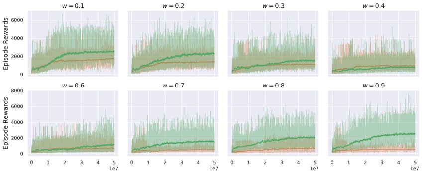
Under review as a conference paper at ICLR 2019

In this paper, we develop an unbiased reward estimator aided robust framework that enables an RL
agent to learn in a noisy environment with observing only perturbed rewards. Our solution frame-
work builds on existing reinforcement learning algorithms, including the recently developed DRL
ones (Q-Learning (Watkins, 1989; Watkins & Dayan, 1992), Cross-Entropy Method (CEM) (Szita
& Lörincz, 2006), Deep SARSA (Sutton & Barto, 1998), Deep Q-Network (DQN) (Mnih et al.,
2013; 2015; van Hasselt et al., 2016), Dueling DQN (DDQN) (Wang et al., 2016), Deep Determin-
istic Policy Gradient (DDPG) (Lillicrap et al., 2015), Continuous DQN (NAF) (Gu et al., 2016) and
Proximal Policy Optimization (PPO) (Schulman et al., 2017) algorithms).
The main challenge is that the observed rewards are likely to be biased, and in RL or DRL the
accumulated errors could amplify the reward estimation error over time. We do not require any
assumption on knowing the true distribution of reward or adversarial strategies, other than the fact
that the generation of noises follow an unknown reward confusion matrix. Instead, we address the
issue of estimating the reward confusion matrices by proposing an efficient and flexible estimation
module. Everitt et al. (2017) provided preliminary studies for the noisy reward problem and gave
some general negative results. The authors proved a No Free Lunch theorem, which is, without
any assumption about what the reward corruption is, all agents can be misled. Our results do not
contradict with the results therein, as we consider a specific noise generation model (that leads to a
set of perturbed rewards). We analyze the convergence and sample complexity for the policy trained
based on our proposed method using surrogate rewards in RL, using Q-Learning as an example.
We conduct extensive experiments on OpenAI Gym (Brockman et al., 2016) (AirRaid, Alien, Car-
nival, MsPacman, Pong, Phoenix, Seaquest) and show that the proposed reward robust RL method
achieves comparable performance with the policy trained using the true rewards. In some cases, our
method even achieves higher cumulative reward - this is surprising to us at first, but we conjecture
that the inserted noise together with our noisy-removal unbiased estimator adds another layer of
exploration, which proves to be beneficial in some settings. This merits a future study.
Our contributions are summarized as follows: (1) We adapt and generalize the idea of defining
a simple but effective unbiased estimator for true rewards using observed and perturbed rewards
to the reinforcement learning setting. The proposed estimator helps guarantee the convergence to
the optimal policy even when the RL agents only have noisy observations of the rewards. (2) We
analyze the convergence to the optimal policy and finite sample complexity of our reward robust RL
methods, using Q-Learning as the running example. (3) Extensive experiments on OpenAI Gym
show that our proposed algorithms perform robustly even at high noise rates.

1.1   R ELATED W ORK

Robust Reinforcement Learning It is known that RL algorithms are vulnerable to noisy envi-
ronments (Irpan, 2018). Recent studies (Huang et al., 2017; Kos & Song, 2017; Lin et al., 2017)
show that learned RL policies can be easily misled with small perturbations in observations. The
presence of noise is very common in real-world environments, especially in robotics-relevant appli-
cations. Consequently, robust (adversarial) reinforcement learning (RRL/RARL) algorithms have
been widely studied, aiming to train a robust policy which is capable of withstanding perturbed
observations (Teh et al., 2017; Pinto et al., 2017; Gu et al., 2018) or transferring to unseen envi-
ronments (Rajeswaran et al., 2016; Fu et al., 2017). However, these robust RL algorithms mainly
focus on noisy vision observations, instead of the observed rewards. A couple of recent works (Lim
et al., 2016; Roy et al., 2017) have also looked into a rather parallel question of training robust RL
algorithms with uncertainty in models.
Learning with Noisy Data Learning appropriately with biased data has received quite a bit of
attention in recent machine learning studies Natarajan et al. (2013); Scott et al. (2013); Scott (2015);
Sukhbaatar & Fergus (2014); van Rooyen & Williamson (2015); Menon et al. (2015). The idea of
above line of works is to define unbiased surrogate loss function to recover the true loss using the
knowledge of the noises. We adapt these approaches to reinforcement learning. Though intuitively
the idea should apply in our RL settings, our work is the first one to formally establish this extension
both theoretically and empirically. Our quantitative understandings will provide practical insights
when implementing reinforcement learning algorithms in noisy environments.

                                                   2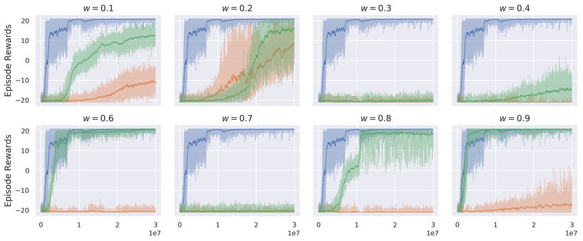
Under review as a conference paper at ICLR 2019

2       P ROBLEM FORMULATION AND PRELIMINARIES

In this section, we define our problem of learning from perturbed rewards in reinforcement learning.
Throughout this paper, we will use perturbed reward and noisy reward interchangeably, as each
time step of our sequential decision making setting is similar to the “learning with noisy data”
setting in supervised learning (Natarajan et al., 2013; Scott et al., 2013; Scott, 2015; Sukhbaatar &
Fergus, 2014). In what follows, we formulate our Markov Decision Process (MDP) problem and the
reinforcement learning (RL) problem with perturbed (noisy) rewards.

2.1     R EINFORCEMENT L EARNING : T HE N OISE -F REE S ETTING

Our RL agent interacts with an unknown environment and attempts to maximize the total of his
collected reward. The environment is formalized as a Markov Decision Process (MDP), denot-
ing as M = hS, A, R, P, γi. At each time t, the agent in state st ∈ S takes an action at ∈ A,
which returns a reward r(st , at , st+1 ) ∈ R (which we will also shorthand as rt ), and leads to
the next state st+1 ∈ S according to a transition probability kernel P, which encodes the proba-
bility Pa (st , st+1 ). Commonly P is unknown to the agent. The agent’s goal is to learn the opti-
mal policy, a conditional distribution π(a|s) that maximizes the state’s value function. The value
function calculates the cumulative reward the agent is expected to receiveP    given he would follow
                                                                                  ∞
the current policy π after observing the current state st : V π (s) = Eπ               k

                                                                                  k=1 γ rt+k | st = s ,
where 0 ≤ γ ≤ 11 is a discount factor. Intuitively, the agent evaluates how preferable each
state is given the currentP policy. From the Bellman Equation, the optimal value function is given
by V ∗ (s) = maxa∈A st+1 ∈S Pa (st , st+1 ) [rt + γV ∗ (st+1 )] . It is a standard practice for RL al-
gorithms to learn a state-action value function, also called the Q-function. Q-function denotes
the expected cumulative reward if agent chooses a in the current state and follows π thereafter:
Qπ (s, a) = Eπ [r(st , at , st+1 ) + γV π (st+1 ) | st = s, at = a] .

2.2     P ERTURBED R EWARD IN RL

In many practical settings, our RL agent does not observe the reward feedback perfectly. We con-
sider the following MDP with perturbed reward, denoting as M̃ = hS, A, R, C, P, γi2 : instead
of observing rt ∈ R at each time t directly (following his action), our RL agent only observes a
perturbed version of rt , denoting as r̃t ∈ R̃. For most of our presentations, we focus on the cases
where R, R̃ are finite sets; but our results generalize to the continuous reward settings.
The generation of r̃ follows a certain function C : S × R → R̃. To let our presentation stay focused,
we consider the following simple state-independent3 flipping error rates model: if the rewards are
binary (consider r+ and r− ), r̃(st , at , st+1 ) (r̃t ) can be characterized by the following noise rate
parameters e+ , e− : e+ = P(r̃(st , at , st+1 ) = r− |r(st , at , st+1 ) = r+ ), e− = P(r̃(st , at , st+1 ) =
r+ |r(st , at , st+1 ) = r− ). When the signal levels are beyond binary, suppose there are M outcomes
in total, denoting as [R0 , R1 , · · · , RM −1 ]. r̃t will be generated according to the following confusion
matrix CM ×M where each entry cj,k indicates the flipping probability for generating a perturbed
outcome: cj,k = P(r̃t = Rk |rt = Rj ). Again we’d like to note that we focus on settings with finite
reward levels for most of our paper, but we provide discussions in Section 3.1 on how to handle
continuous rewards with discretizations.
In the paper, we do not assume knowing the noise rates (i.e., the reward confusion matrices), which
is different from the assumption of knowing them as adopted in many supervised learning works
Natarajan et al. (2013). Instead we will estimate the confusion matrices (Section 3.3).

    1
     γ = 1 indicates an undiscounted MDP setting (Schwartz, 1993; Sobel, 1994; Kakade, 2003).
    2
     The MDP with perturbed reward can equivalently be defined as a tuple M̃ = hS, A, R, R̃, P, γi, with the
perturbation function C implicitly defined as the difference between R and R̃.
   3
     The case of state-dependent perturbed reward is discussed in Appendix C.3

                                                         3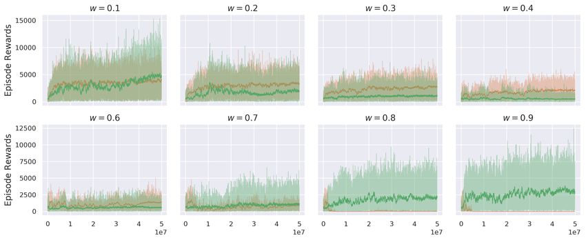
Under review as a conference paper at ICLR 2019

3     L EARNING WITH P ERTURBED R EWARDS
In this section, we first introduce an unbiased estimator for binary rewards in our reinforcement
learning setting when the error rates are known. This idea is inspired by Natarajan et al. (2013), but
we will extend the method to the multi-outcome, as well as the continuous reward settings.

3.1   U NBIASED E STIMATOR FOR T RUE R EWARD

With the knowledge of noise rates (reward confusion matrices), we are able to establish an unbiased
approximation of the true reward in a similar way as done in Natarajan et al. (2013). We will
call such a constructed unbiased reward as a surrogate reward. To give an intuition, we start with
replicating the results for binary reward R = {r− , r+ } in our RL setting:
Lemma 1. Let r be bounded. Then, if we define,
                                                 ( (1−e− )·r+ −e+ ·r−
                                                       1−e+ −e−
                                                                            (r̃(st , at , st+1 ) = r+ )
                        r̂(st , at , st+1 ) :=     (1−e+ )·r− −e− ·r+                                          (1)
                                                       1−e+ −e−
                                                                            (r̃(st , at , st+1 ) = r− )
we have for any r(st , at , st+1 ), Er̃|r [r̂(st , at , st+1 )] = r(st , at , st+1 ).
In the standard supervised learning setting, the above property guarantees convergence - as more
training data are collected, the empirical surrogate risk converges to its expectation, which is the
same as the expectation of the true risk (due to unbiased estimators). This is also the intuition why
we would like to replace the reward terms with surrogate rewards in our RL algorithms.
The above idea can be generalized to the multi-outcome setting in a fairly straight-forward way.
Define R̂ := [r̂(r̃ = R0 ), r̂(r̃ = R1 ), ..., r̂(r̃ = RM −1 )], where r̂(r̃ = Rm ) denotes the value of the
surrogate reward when the observed reward is Rk . Let R = [R0 ; R1 ; · · · ; RM −1 ] be the bounded
reward matrix with M values. We have the following results:
Lemma 2. Suppose CM ×M is invertible. With defining:
                                                       R̂ = C−1 · R.                                           (2)
we have for any r(st , at , st+1 ), Er̃|r [r̂(st , at , st+1 )] = r(st , at , st+1 ).
Continuous reward When the reward signal is continuous, we discretize it into M intervals and
view each interval as a reward level, with its value approximated by its middle point. With increasing
M , this quantization error can be made arbitrarily small. Our method is then the same as the solution
for the multi-outcome setting, except for replacing rewards with discretized ones. Note that the finer-
degree quantization we take, the smaller the quantization error - but we would suffer from learning
a bigger reward confusion matrix. This is a trade-off question that can be addressed empirically.
So far we have assumed knowing the confusion matrices, but we will address this additional estima-
tion issue in Section 3.3, and present our complete algorithm therein.

3.2   C ONVERGENCE AND S AMPLE C OMPLEXITY: Q-L EARNING

We now analyze the convergence and sample complexity of our surrogate reward based RL algo-
rithms (with assuming knowing C), taking Q-Learning as an example.
Convergence guarantee First, the convergence guarantee is stated in the following theorem:
Theorem 1. Given a finite MDP, denoting as M̂ = hS, A, R̂, P, γi, the Q-learning algorithm with
surrogate rewards, given by the update rule,

                      Qt+1 (st , at ) = (1 − αt )Q(st , at ) + αt r̂t + γ max Q(st+1 , b) ,                    (3)
                                                                                    b∈A

                                                                                                    αt2 < ∞.
                                                                   P                         P
converges w.p.1 to the optimal Q-function as long as                    t   αt = ∞ and          t

Note that the term on the right hand of Eqn. (3) includes surrogate reward r̂ estimated using Eqn. (1)
and Eqn. (2). Theorem 1 states that that agents will converge to the optimal policy w.p.1 with
replacing the rewards with surrogate rewards, despite of the noises in observing rewards. This result
is not surprising - though the surrogate rewards introduce larger variance, we are grateful of their
unbiasedness, which grants us the convergence. In other words, the addition of the perturbed reward
does not destroy the convergence guarantees of Q-Learning.

                                                              4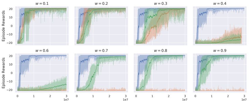
Under review as a conference paper at ICLR 2019

Sample complexity To establish our sample complexity results, we first introduce a generative
model following previous literature (Kearns & Singh, 1998; 2000; Kearns et al., 1999). This is a
practical MDP setting to simplify the analysis.
Definition 1. A generative model G(M) for an MDP M is a sampling model which takes a state-
action pair (st , at ) as input, and outputs the corresponding reward r(st , at ) and the next state st+1
randomly with the probability of Pa (st , st+1 ), i.e., st+1 ∼ P(·|s, a).
Exact value iteration is impractical if the agents follow the generative models above exactly (Kakade,
2003). Consequently, we introduce a phased Q-Learning which is similar to the ones presented
in Kakade (2003); Kearns & Singh (1998) for the convenience of proving our sample complexity
results. We briefly outline phased Q-Learning as follows - the complete description (Algorithm 2)
can be found in Appendix A.
Definition 2. Phased Q-Learning algorithm takes m samples per phase by calling generative model
G(M). It uses the collected m samples to estimate the transition probability P and update the
estimated value function per phase. Calling generative model G(M̂) means that surrogate rewards
are returned and used to update value function per phase.
The sample complexity of Phased Q-Learning is given as follows:
Theorem 2. (Upper Bound) Let r ∈ [0, Rmax ] be bounded reward, C be an invertible reward
confusion matrix with det(C) denoting its determinant. For anappropriate choice of m, the
                                                                                          Phased
                                                                  |S||A|T        |S||A|T
Q-Learning algorithm calls the generative model G(M̂) O 2 (1−γ)2 det(C)2 log δ            times in
T epochs, and returns a policy such that for all state s ∈ S, |Vπ (s) − V ∗ (s)| ≤ ,  > 0, w.p.
≥ 1 − δ, 0 < δ < 1.
Theorem 2 states that, to guarantee the convergence to the optimal policy, the number of samples
needed is no more than O(1/det(C)2 ) times of the one needed when the RL agent observes true
rewards perfectly. This additional constant is the price we pay for the noise presented in our learning
environment. When the noise level is high, we expect to see a much higher 1/det(C)2 ; otherwise
when we are in a low-noise regime , Q-Learning can be very efficient with surrogate reward (Kearns
& Singh, 2000). Note that Theorem 2 gives the upper bound in discounted MDP setting;          for undis-
                                                                           3
counted setting (γ = 1), the upper bound is at the order of O |S||A|T
                                                                    2 det(C)2 log |S||A|T
                                                                                      δ     . Lower bound
result is omitted due to the lack of space. Theidea of constructing MDP in which learning is difficult
and the algorithm must make |S||A|T       log 1δ calls to G(M̂), is similar to Kakade (2003).

While the surrogate reward guarantees the unbiasedness, we sacrifice the variance at each of our
learning steps, and this in turn delays the convergence (as also evidenced in the sample complexity
bound). It can be verified that the variance of surrogate reward is bounded when C is invertible, and
it is always higher than the variance of true reward. This is summarized in the following theorem:
Theorem 3. Let r ∈ [0, Rmax ] be bounded reward and confusion matrix C is invertible. Then, the
                                                                                 M2       2
variance of surrogate reward r̂ is bounded as follows: Var(r) ≤ Var(r̂) ≤ det(C)     2 · Rmax .

To give an intuition of the bound, when we have binary reward, the variance for surrogate reward
                                                4R2
bounds as follows: Var(r) ≤ Var(r̂) ≤ (1−e+max     −e− )2 . As e− + e+ → 1, the variance becomes
unbounded and the proposed estimator is no longer effective, nor will it be well-defined. In practice,
there is a trade-off question between bias and variance by tuning a linear combination of R and R̂,
i.e., Rproxy = ηR + (1 − η)R̂, and choosing an appropriate η ∈ [0, 1].

3.3   E STIMATION OF C ONFUSION M ATRICES

In Section 3.1 we have assumed the knowledge of reward confusion matrices, in order to compute
the surrogate reward. This knowledge is often not available in practice. Estimating these confusion
matrices is challenging without knowing any ground truth reward information; but we’d like to note
that efficient algorithms have been developed to estimate the confusion matrices in supervised learn-
ing settings (Bekker & Goldberger, 2016; Liu & Liu, 2017; Khetan et al., 2017; Hendrycks et al.,
2018). The idea in these algorithms is to dynamically refine the error rates based on aggregated re-
wards. Note this approach is not different from the inference methods in aggregating crowdsourcing

                                                    5
Under review as a conference paper at ICLR 2019

labels, as referred in the literature (Dawid & Skene, 1979; Karger et al., 2011; Liu et al., 2012). We
adapt this idea to our reinforcement learning setting, which is detailed as follows.
At each training step, the RL agent collects the noisy reward and the current state-action pair. Then,
for each pair in S × A, the agent predicts the true reward based on accumulated historical observa-
tions of reward for the corresponding state-action pair via, e.g., averaging (majority voting). Finally,
with the predicted true reward and the accuracy (error rate) for each state-action pair, the estimated
reward confusion matrices C̃ are given by
                                        P
                                        (s,a)∈S×A     # [r̃(s, a) = Rj |r̄(s, a) = Ri ]
                              c̃i,j =          P                                          ,                      (4)
                                                  (s,a)∈S×A    #[r̄(s, a) = Ri ]

 where in above # [·] denotes the number of state-action pair that satisfies the condition [·] in the
set of observed rewards R̃(s, a) (see Algorithm 1 and 3); r̄(s, a) and r̃(s, a) denote predicted true
rewards (using majority voting) and observed rewards when the state-action pair is (s, a). The above
procedure of updating c̃i,j continues indefinitely as more observation arrives.
Our final definition of surrogate           Algorithm 1 Reward Robust RL (sketch)
reward replaces a known reward
confusion C in Eqn. (2) with our            Input: M̃, α, β, R̃(s, a)
                                            Output: Q(s), π(s, t)
estimated one C̃. We denote this              Initialize value function Q(s, a) arbitrarily.
estimated surrogate reward as ṙ.             while Q is not converged do
We present (Reward Robust RL)                     Initialize state s ∈ S
in Algorithm 14 . Note that the                   while s is not terminal do
                                                       Choose a from s using policy derived from Q
algorithm is rather generic, and                       Take action a, observe s0 and noisy reward r̃
we can plug in any exisitng RL                         if collecting enough r̃ for every S × A pair then
algorithm into our reward robust                           Get predicted true reward r̄ using majority voting
one, with only changes in re-                              Estimate confusion matrix C̃ based on r̃ and r̄ (Eqn. 4)
placing the rewards with our es-                       Obtain surrogate reward ṙ (R̂ = (1 − η) · R + η · C−1 R)
timated surrogate rewards.                             Update Q using surrogate reward
                                                       s ← s0
                                              return Q(s) and π(s)
4       E XPERIMENTS

In this section, reward robust RL is tested in different games, with different noise settings. Due to
space limit, more experimental results can be found in Appendix D.

4.1       E XPERIMENTAL S ETUP

Environments and RL Algorithms To fully test the performance under different environments,
we evaluate the proposed robust reward RL method on two classic control games (CartPole, Pendu-
lum) and seven Atari 2600 games (AirRaid, Alien, Carnival, MsPacman, Pong, Phoenix, Seaquest),
which encompass a large variety of environments, as well as rewards. Specifically, the rewards
could be unary (CartPole), binary (most of Atari games), multivariate (Pong) and even continu-
ous (Pendulum). A set of state-of-the-art reinforcement learning algorithms are experimented with
while training under different amounts of noise (See Table 3)5 . For each game and algorithm, three
policies are trained based on different random initialization to decrease the variance.

Reward Post-Processing For each game and RL algorithm, we test the performances for learning
with true rewards, learning with noisy rewards and learning with surrogate rewards. Both symmet-
ric and asymmetric noise settings with different noise levels are tested. For symmetric noise, the
confusion matrices are symmetric. As for asymmetric noise, two types of random noise are tested:
1) rand-one, each reward level can only be perturbed into another reward; 2) rand-all, each reward
could be perturbed to any other reward, via adding a random noise matrix. To measure the amount
of noise w.r.t confusion matrices, we define the weight of noise ω in Appendix B.2. The larger ω is,
the higher the noise rates are.
    4
        One complete Q-Learning implementation (Algorithm 3) is provided in Appendix C.1.
    5
        The detailed settings are accessible in Appendix B.

                                                           6
Under review as a conference paper at ICLR 2019

4.2        ROBUSTNESS E VALUATION

CartPole The goal in CartPole is to prevent the pole from falling by controlling the cart’s direction
and velocity. The reward is +1 for every step taken, including the termination step. When the cart or
pole deviates too much or the episode length is longer than 200, the episode terminates. Due to the
unary reward {+1} in CartPole, a corrupted reward −1 is added as the unexpected error (e− = 0).
As a result, the reward space R is extended to {+1, −1}. Five algorithms Q-Learning (1992),
CEM (2006), SARSA (1998), DQN (2016) and DDQN (2016) are evaluated.
ω = 0.3
ω = 0.7

          (a) Q-Learning          (b) CEM         (c) SARSA            (d) DQN            (e) DDQN

Figure 1: Learning curves from five RL algorithms on CartPole game with true rewards (r) , noisy
rewards (r̃) and estimated surrogate rewards (ṙ) (η = 1) . Note that reward confusion matrices
C are unknown to the agents here. Full results are in Appendix D.2 (Figure 6).
In Figure 1, we show that our estimator successfully produces meaningful surrogate rewards that
adapt the underlying RL algorithms to the noisy settings, without any assumption of the true distri-
bution of rewards. With the noise rate increasing (from 0.1 to 0.9), the models with noisy rewards
converge slower due to larger biases. However, we observe that the models always converge to the
best score 200 with the help of surrogate rewards.
In some circumstances (slight noise - see Figure 6a, 6b, 6c, 6d), the surrogate rewards even lead to
faster convergence. This points out an interesting observation: learning with surrogate reward even
outperforms the case with observing the true reward. We conjecture that the way of adding noise
and then removing the bias introduces implicit exploration. This implies that for settings even with
true reward, we might consider manually adding noise and then remove it in expectation.

Pendulum The goal in Pendulum is to keep a frictionless pendulum standing up. Different from
the CartPole setting, the rewards in pendulum are continuous: r ∈ (−16.28, 0.0]. The closer the
reward is to zero, the better performance the model achieves. Following our extension (see Sec-
tion 3.1), the (−17, 0] is firstly discretized into 17 intervals: (−17, −16], (−16, −15], · · · , (−1, 0],
with its value approximated using its maximum point. After the quantization step, the surrogate
rewards can be estimated using multi-outcome extensions presented in Section 3.1.
Table 1: Average scores of various RL algorithms on CartPole and Pendulum with noisy rewards (r̃)
and surrogate rewards under known (r̂) or estimated (ṙ) noise rates. Note that the results for last two
algorithms DDPG (rand-one) & NAF (rand-all) are on Pendulum, but the others are on CartPole.

             Noise Rate    Reward    Q-Learn   CEM     SARSA   DQN      DDQN     DDPG      NAF
                             r̃       170.0     98.1   165.2   187.2    187.8     -1.03    -4.48
               ω = 0.1       r̂       165.8    108.9   173.6   200.0    181.4     -0.87    -0.89
                             ṙ       181.9    99.3    171.5   200.0    185.6     -0.90    -1.13
                             r̃       134.9    28.8    144.4   173.4    168.6     -1.23    -4.52
               ω = 0.3       r̂       149.3    85.9    152.4   175.3    198.7     -1.03    -1.15
                             ṙ       161.1    82.2    159.6   186.7    200.0     -1.05    -1.36

We experiment two popular algorithms, DDPG (2015) and NAF (2016) in this game. In Figure 2,
both algorithms perform well with surrogate rewards under different amounts of noise. In most
cases, the biases were corrected in the long-term, even when the amount of noise is extensive (e.g.,
ω = 0.7). The quantitative scores on CartPole and Pendulum are given in Table 1, where the

                                                       7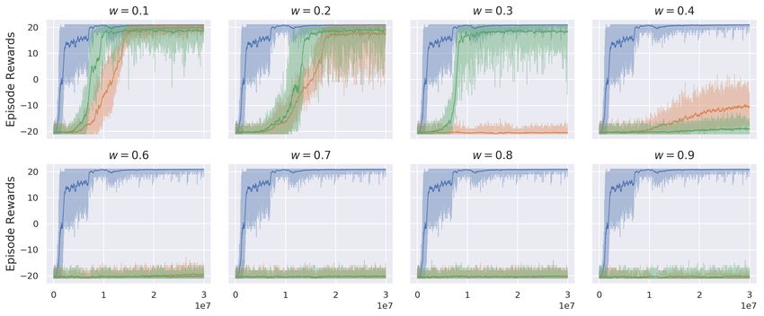
Under review as a conference paper at ICLR 2019
ω = 0.3
ω = 0.7
(a) DDPG (symmetric) (b) DDPG (rand-one) (c) DDPG (rand-all) (d) NAF (rand-all)
Figure 2: Learning curves from DDPG and NAF on Pendulum game with true rewards (r) , noisy
rewards (r̃) and surrogate rewards (r̂) (η = 1) . Both symmetric and asymmetric noise are
conduced in the experiments. Full results are in Appendix D.2 (Figure 8).
scores are averaged based on the last thirty episodes. The full results (ω > 0.5) can be found in
Appendix D.1, so does Table 2. Our reward robust RL method is able to achieve consistently good
scores.
Atari We validate our algorithm on seven Atari 2600 games using the state-of-the-art algorithm
PPO (Schulman et al., 2017). The games are chosen to cover a variety of environments. The rewards
in the Atari games are clipped into {−1, 0, 1}. We leave the detailed settings to Appendix B.
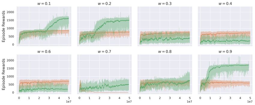
Figure 3: Learning curves from PPO on Pong-v4 game with true rewards (r) , noisy rewards (r̃)
and surrogate rewards (η = 1) (r̂) . The noise rates increase from 0.1 to 0.9, with a step of 0.1.
Results for PPO on Pong-v4 in symmetric noise setting are presented in Figure 3. Due to limited
space, more results on other Atari games and noise settings are given in Appendix D.3. Similar to
previous results, our surrogate estimator performs consistently well and helps PPO converge to the
optimal policy. Table 2 shows the average scores of PPO on five selected Atari games with different
amounts of noise (symmetric & asymmetric). In particular, when the noise rates e+ = e− > 0.3,
agents with surrogate rewards obtain significant amounts of improvements in average scores. We do
not present the results for the case with unknown C because the state-space (image-input) is very
large for Atari games, which is difficult to handle with the solution given in Section 3.3.
5 C ONCLUSION
Only an underwhelming amount of reinforcement learning studies have focused on the settings with
perturbed and noisy rewards, despite the fact that such noises are common when exploring a real-
world scenario, that faces sensor errors or adversarial examples. We adapt the ideas from supervised
8
Under review as a conference paper at ICLR 2019

Table 2: Average scores of PPO on five selected games with noisy rewards (r̃) and surrogate rewards
(r̂). The experiments are repeated three times with different random seeds.

       Noise Rate        Reward   Lift (↑)   Mean         Alien   Carnival   Phoenix   MsPacman   Seaquest
                           r̃        -       2044.2   1814.8      1239.2     4608.9     1709.1     849.2
      e− = e+ = 0.1
                           r̂     67.5%↑     3423.1   1741.0      3630.3     7586.3     2547.3    1610.6
                           r̃        -       770.5        893.3    841.8      250.7     1151.1     715.7
    e− = 0.1, e+ = 0.3
                           r̂     20.3%↑     926.6        973.7    955.2      643.9     1307.1     753.1
                           r̃        -       1180.1    543.1       919.8     2600.3     1109.6     727.8
      e− = e+ = 0.3
                           r̂     46.7%↑     1730.8   1637.7       966.1     4171.5     1470.2     408.6

learning with noisy examples (Natarajan et al., 2013), and propose a simple but effective RL frame-
work for dealing with noisy rewards. The convergence guarantee and finite sample complexity of
Q-Learning (or its variant) with estimated surrogate rewards are given. To validate the effective-
ness of our approach, extensive experiments are conducted on OpenAI Gym, showing that surrogate
rewards successfully rescue models from misleading rewards even at high noise rates.

R EFERENCES
Alan Joseph Bekker and Jacob Goldberger. Training deep neural-networks based on unreliable
  labels. In ICASSP, pp. 2682–2686. IEEE, 2016.

Greg Brockman, Vicki Cheung, Ludwig Pettersson, Jonas Schneider, John Schulman, Jie Tang, and
  Wojciech Zaremba. Openai gym, 2016.

Alexander Philip Dawid and Allan M Skene. Maximum likelihood estimation of observer error-rates
  using the em algorithm. Applied statistics, pp. 20–28, 1979.

Prafulla Dhariwal, Christopher Hesse, Oleg Klimov, Alex Nichol, Matthias Plappert, Alec Radford,
  John Schulman, Szymon Sidor, and Yuhuai Wu. Openai baselines. https://github.com/
  openai/baselines, 2017.

Tom Everitt, Victoria Krakovna, Laurent Orseau, and Shane Legg. Reinforcement learning with a
  corrupted reward channel. In IJCAI, pp. 4705–4713. ijcai.org, 2017.

Justin Fu, Katie Luo, and Sergey Levine. Learning robust rewards with adversarial inverse rein-
  forcement learning. CoRR, abs/1710.11248, 2017.

Shixiang Gu, Timothy P. Lillicrap, Ilya Sutskever, and Sergey Levine. Continuous deep q-learning
  with model-based acceleration. In ICML, volume 48 of JMLR Workshop and Conference Pro-
  ceedings, pp. 2829–2838. JMLR.org, 2016.

Zhaoyuan Gu, Zhenzhong Jia, and Howie Choset. Adversary a3c for robust reinforcement learning,
  2018. URL https://openreview.net/forum?id=SJvrXqvaZ.

Dylan Hadfield-Menell, Smitha Milli, Pieter Abbeel, Stuart J Russell, and Anca Dragan. Inverse
  reward design. In Advances in Neural Information Processing Systems, pp. 6765–6774, 2017.

Dan Hendrycks, Mantas Mazeika, Duncan Wilson, and Kevin Gimpel. Using trusted data to train
  deep networks on labels corrupted by severe noise. CoRR, abs/1802.05300, 2018.

Sandy Huang, Nicolas Papernot, Ian Goodfellow, Yan Duan, and Pieter Abbeel. Adversarial attacks
  on neural network policies. arXiv preprint arXiv:1702.02284, 2017.

Alex Irpan. Deep reinforcement learning doesn’t work yet. https://www.alexirpan.com/
  2018/02/14/rl-hard.html, 2018.

Tommi S. Jaakkola, Michael I. Jordan, and Satinder P. Singh. Convergence of stochastic iterative
  dynamic programming algorithms. In NIPS, pp. 703–710. Morgan Kaufmann, 1993.

                                                      9
Under review as a conference paper at ICLR 2019

Sham Machandranath Kakade. On the Sample Complexity of Reinforcement Learning. PhD thesis,
  University of London, 2003.
David R Karger, Sewoong Oh, and Devavrat Shah. Iterative learning for reliable crowdsourcing
  systems. In Advances in neural information processing systems, pp. 1953–1961, 2011.
Michael J. Kearns and Satinder P. Singh. Finite-sample convergence rates for q-learning and indirect
 algorithms. In NIPS, pp. 996–1002. The MIT Press, 1998.
Michael J. Kearns and Satinder P. Singh. Bias-variance error bounds for temporal difference updates.
 In COLT, pp. 142–147. Morgan Kaufmann, 2000.
Michael J. Kearns, Yishay Mansour, and Andrew Y. Ng. A sparse sampling algorithm for near-
 optimal planning in large markov decision processes. In IJCAI, pp. 1324–1231. Morgan Kauf-
 mann, 1999.
Ashish Khetan, Zachary C. Lipton, and Anima Anandkumar. Learning from noisy singly-labeled
  data. CoRR, abs/1712.04577, 2017.
Jernej Kos and Dawn Song.          Delving into adversarial attacks on deep policies.        CoRR,
   abs/1705.06452, 2017.
Timothy P. Lillicrap, Jonathan J. Hunt, Alexander Pritzel, Nicolas Heess, Tom Erez, Yuval Tassa,
  David Silver, and Daan Wierstra. Continuous control with deep reinforcement learning. CoRR,
  abs/1509.02971, 2015.
Shiau Hong Lim, Huan Xu, and Shie Mannor. Reinforcement learning in robust markov decision
  processes. Math. Oper. Res., 41(4):1325–1353, 2016.
Yen-Chen Lin, Zhang-Wei Hong, Yuan-Hong Liao, Meng-Li Shih, Ming-Yu Liu, and Min Sun.
  Tactics of adversarial attack on deep reinforcement learning agents. In IJCAI, pp. 3756–3762.
  ijcai.org, 2017.
Qiang Liu, Jian Peng, and Alexander T Ihler. Variational inference for crowdsourcing. In Proc. of
  NIPS, 2012.
Yang Liu and Mingyan Liu. An online learning approach to improving the quality of crowd-
  sourcing. IEEE/ACM Transactions on Networking, 25(4):2166–2179, Aug 2017.
R. Loftin, B. Peng, J. MacGlashan, M. L. Littman, M. E. Taylor, J. Huang, and D. L. Roberts.
  Learning something from nothing: Leveraging implicit human feedback strategies. In The 23rd
  IEEE International Symposium on Robot and Human Interactive Communication, pp. 607–612,
  Aug 2014.
Aditya Menon, Brendan Van Rooyen, Cheng Soon Ong, and Bob Williamson. Learning from cor-
  rupted binary labels via class-probability estimation. In International Conference on Machine
  Learning, pp. 125–134, 2015.
Volodymyr Mnih, Koray Kavukcuoglu, David Silver, Alex Graves, Ioannis Antonoglou, Daan
  Wierstra, and Martin A. Riedmiller. Playing atari with deep reinforcement learning. CoRR,
  abs/1312.5602, 2013.
Volodymyr Mnih, Koray Kavukcuoglu, David Silver, Andrei A Rusu, Joel Veness, Marc G Belle-
  mare, Alex Graves, Martin Riedmiller, Andreas K Fidjeland, Georg Ostrovski, et al. Human-level
  control through deep reinforcement learning. Nature, 518(7540):529, 2015.
Nagarajan Natarajan, Inderjit S Dhillon, Pradeep K Ravikumar, and Ambuj Tewari. Learning with
  noisy labels. In Advances in neural information processing systems, pp. 1196–1204, 2013.
Lerrel Pinto, James Davidson, Rahul Sukthankar, and Abhinav Gupta. Robust adversarial rein-
  forcement learning. In ICML, volume 70 of Proceedings of Machine Learning Research, pp.
  2817–2826. PMLR, 2017.
Matthias Plappert. keras-rl. https://github.com/keras-rl/keras-rl, 2016.

                                                10
Under review as a conference paper at ICLR 2019
Aravind Rajeswaran, Sarvjeet Ghotra, Sergey Levine, and Balaraman Ravindran. Epopt: Learning
robust neural network policies using model ensembles. CoRR, abs/1610.01283, 2016.
Joshua Romoff, Alexandre Piché, Peter Henderson, Vincent François-Lavet, and Joelle Pineau. Re-
ward estimation for variance reduction in deep reinforcement learning. CoRR, abs/1805.03359,
2018.
Aurko Roy, Huan Xu, and Sebastian Pokutta. Reinforcement learning under model mismatch.
CoRR, abs/1706.04711, 2017.
John Schulman, Filip Wolski, Prafulla Dhariwal, Alec Radford, and Oleg Klimov. Proximal policy
optimization algorithms. CoRR, abs/1707.06347, 2017.
Anton Schwartz. A reinforcement learning method for maximizing undiscounted rewards. In ICML,
pp. 298–305. Morgan Kaufmann, 1993.
Clayton Scott. A rate of convergence for mixture proportion estimation, with application to learning
from noisy labels. In AISTATS, 2015.
Clayton Scott, Gilles Blanchard, Gregory Handy, Sara Pozzi, and Marek Flaska. Classification with
asymmetric label noise: Consistency and maximal denoising. In COLT, pp. 489–511, 2013.
Matthew J. Sobel. Mean-variance tradeoffs in an undiscounted MDP. Operations Research, 42(1):
175–183, 1994.
Sainbayar Sukhbaatar and Rob Fergus. Learning from noisy labels with deep neural networks. arXiv
preprint arXiv:1406.2080, 2(3):4, 2014.
Richard S. Sutton and Andrew G. Barto. Reinforcement learning - an introduction. Adaptive com-
putation and machine learning. MIT Press, 1998.
Istvan Szita and András Lörincz. Learning tetris using the noisy cross-entropy method. Neural
Computation, 18(12):2936–2941, 2006.
Yee Whye Teh, Victor Bapst, Wojciech M. Czarnecki, John Quan, James Kirkpatrick, Raia Hadsell,
Nicolas Heess, and Razvan Pascanu. Distral: Robust multitask reinforcement learning. In NIPS,
pp. 4499–4509, 2017.
Andrea Lockerd Thomaz, Cynthia Breazeal, et al. Reinforcement learning with human teachers:
Evidence of feedback and guidance with implications for learning performance. 2006.
John N. Tsitsiklis. Asynchronous stochastic approximation and q-learning. Machine Learning, 16
(3):185–202, 1994.
Hado van Hasselt, Arthur Guez, and David Silver. Deep reinforcement learning with double q-
learning. In AAAI, pp. 2094–2100. AAAI Press, 2016.
Brendan van Rooyen and Robert C Williamson. Learning in the presence of corruption. arXiv
preprint arXiv:1504.00091, 2015.
Ziyu Wang, Tom Schaul, Matteo Hessel, Hado van Hasselt, Marc Lanctot, and Nando de Freitas.
Dueling network architectures for deep reinforcement learning. In ICML, volume 48 of JMLR
Workshop and Conference Proceedings, pp. 1995–2003. JMLR.org, 2016.
Christopher J. C. H. Watkins and Peter Dayan. Q-learning. In Machine Learning, pp. 279–292,
1992.
Christopher John Cornish Hellaby Watkins. Learning from Delayed Rewards. PhD thesis, King’s
College, Cambridge, UK, May 1989.
Yuchen Zhang, Xi Chen, Denny Zhou, and Michael I Jordan. Spectral methods meet em: A provably
optimal algorithm for crowdsourcing. In Advances in neural information processing systems, pp.
1260–1268, 2014.
11Under review as a conference paper at ICLR 2019
A P ROOFS
Proof of Lemma 1. For simplicity, we shorthand r̂(st , at , st+1 ), r̃(st , at , st+1 ), r(st , at , st+1 ) as
r̂, r̃, r, and let r+ , r− , r̂+ , r̂− denote the general reward levels and corresponding surrogate ones:
Er̃|r (r̂) = Pr̃|r (r̂ = r̂− )r̂− + Pr̃|r (r̂ = r̂+ )r̂+ . (5)
When r = r+ , from the definition in Lemma 1:
Pr̃|r (r̂ = r̂− ) = e+ , Pr̃|r (r̂ = r̂+ ) = 1 − e+ .
Taking the definition of surrogate rewards Eqn. (1) into Eqn. (5), we have
Er̃|r (r̂) = e+ · r̂− + (1 − e+ ) · r̂+
(1 − e+ )r− − e− r+ (1 − e− )r+ − e+ r−
= e+ · + (1 − e+ ) · = r+ .
1 − e− − e+ 1 − e− − e+
Similarly, when r = r− , it also verifies Er̃|r [r̂(st , at , st+1 )] = r(st , at , st+1 ).
Proof of Lemma 2. The idea of constructing unbiased estimator is easily adapted to multi-outcome
reward settings via writing out the conditions for the unbiasedness property (s.t. Er̃|r [r̂] = r.). For
simplicity, we shorthand r̂(r̃ = Ri ) as R̂i in the following proofs. Similar to Lemma 1, we need to
solve the following set of functions to obtain r̂:
R0 = c0,0 · R̂0 + c0,1 · R̂1 + · · · + c0,M −1 · R̂M −1
R1 = c1,0 · R̂0 + c1,1 · R̂1 + · · · + c1,M −1 · R̂M −1
···
RM −1 = cM −1,0 · R̂0 + cM −1,1 · R̂1 + · · · + cM −1,M −1 · R̂M −1
where R̂i denotes the value of the surrogate reward when the observed reward is Ri . Define R :=
[R0 ; R1 ; · · · ; RM −1 ], and R̂ := [R̂0 , R̂1 , ..., R̂M −1 ], then the above equations are equivalent to:
R = C · R̂. If the confusion matrix C is invertible, we obtain the surrogate reward:
R̂ = C−1 · R.
According to above definition, for any true reward level Ri , i = 0, 1, · · · , M − 1, we have
Er̃|r=Ri [r̂] = ci,0 · R̂0 + ci,1 · R̂1 + · · · + ci,M −1 · R̂M −1 = Ri .
Furthermore, the probabilities for observing surrogate rewards can be written as follows:
X X X
P̂ = [p̂1 , p̂2 , · · · , p̂M ] = pj cj,1 , pj cj,2 , · · · , pj cj,M ,
j j j
P
where p̂i = j pj cj,i , and p̂i , pi represent the probabilities of occurrence for surrogate reward R̂i
and true reward Ri respectively.
Corollary 1. Let p̂i and pi denote the probabilities of occurrence for surrogate reward r̂(r̃ = Ri )
and true reward Ri . Then the surrogate reward satisfies,
X X X
Pa (st , st+1 )r(st , a, st+1 ) = pj Rj = p̂j R̂j . (6)
s0 ∈S j j
Proof of Corollary 1. From Lemma 2, we have,
X X
Pa (st , st+1 )r(st , a, st+1 ) = Pa (st , st+1 , Rj )Rj
st ∈S st+1 ∈S;Rj ∈R
X X X X
= Pa (st , st+1 )Rj = pj Rj = pj Rj .
Rj ∈R st+1 ∈S Rj ∈R j
12Under review as a conference paper at ICLR 2019
Consequently,
X XX X X
p̂j R̂j = pk ck,j R̂j = pk ck,j R̂j
j j k k j
X X
= p k Rk = Pa (st , st+1 )r(st , a, st+1 ).
k st ∈S
To establish Theorem 1, we need an auxiliary result (Lemma 3) from stochastic process approxi-
mation, which is widely adopted for the convergence proof for Q-Learning (Jaakkola et al., 1993;
Tsitsiklis, 1994).
Lemma 3. The random process {∆t } taking values in Rn and defined as
∆t+1 (x) = (1 − αt (x))∆t (x) + αt (x)Ft (x)
converges to zero w.p.1 under the following assumptions:
• 0 ≤ αt ≤ 1, t αt (x) = ∞ and t αt (x)2 < ∞;
P P
• ||E [Ft (x)|Ft ] ||W ≤ γ||∆t ||, with γ < 1;
• var [Ft (x)|Ft ] ≤ C(1 + ||∆t ||2W ), for C > 0.
Here Ft = {∆t , ∆t−1 , · · · , Ft−1 · · · , αt , · · · } stands for the past at step t, αt (x) is allowed to
depend on the past insofar as the above conditions remain valid. The notation || · ||W refers to some
weighted maximum norm.
Proof of Lemma 3. See previous literature (Jaakkola et al., 1993; Tsitsiklis, 1994).
Proof of Theorem 1. For simplicity, we abbreviate st , st+1 , Qt , Qt+1 , rt , r̂t and αt as s, s0 , Q, Q0 ,
r, r̂, and α, respectively.
Subtracting from both sides the quantity Q∗ (s, a) in Eqn. (3):
Q0 (s, a) − Q∗ (s, a) = (1 − α) (Q(s, a) − Q∗ (s, a)) + α r̂ + γ max Q(s0 , b) − Q∗ (s, a) .
b∈A
Let ∆t (s, a) = Q(s, a) − Q (s, a) and Ft (s, a) = r̂ + γ maxb∈A Q(s0 , b) − Q∗ (s, a).
∗
∆t+1 (s0 , a) = (1 − α)∆t (s, a) + αFt (s, a).
In consequence,
X
E [Ft (x)|Ft ] = Pa (s, s , r̂) r̂ + γ max Q(s , b) − Q∗ (s, a)
0 0
b∈A
s0 ∈S;r̂∈R
X X
0 0 0 ∗ 0
= Pa (s, s , r̂)r̂ + Pa (s, s ) γ max Q(s , b) − r − γ max Q (s , b)
b∈A b∈A
s0 ∈S;r̂∈R s0 ∈S
X X X
= Pa (s, s0 , r̂)r̂ − Pa (s, s0 )r + Pa (s, s0 )γ max Q(s0 , b) − max Q∗ (s0 , b)
b∈A b∈A
s0 ∈S;r̂∈R s0 ∈S s0 ∈S
X X X
= p̂j r̂j − Pa (s, s0 )r + Pa (s, s0 )γ max Q(s0 , b) − max Q∗ (s0 , b)
b∈A b∈A
j s0 ∈S s0 ∈S
X
= Pa (s, s0 )γ max Q(s0 , b) − max Q∗ (s0 , b) (using Eqn. (6))
b∈A b∈A
s0 ∈S
X
≤γ Pa (s, s0 ) max
0
|Q(s0 , b) − Q∗ (s0 , b)|
b∈A,s ∈S
s0 ∈S
X
=γ Pa (s, s0 )||Q − Q∗ ||∞ = γ||Q − Q∗ ||∞ = γ||∆t ||∞ .
s0 ∈S
13Under review as a conference paper at ICLR 2019
Finally,
X 2
Var [Ft (x)|Ft ] = E r̂ + γ max Q(s0 , b) − P0 (s, s0 , r̂) r̂ + γ max Q(s0 , b)
b∈A b∈A
s0 ∈S;r̂∈R
= Var r̂ + γ max Q(s0 , b)|Ft
b∈A
.
Because r̂ is bounded, it can be clearly verified that
Var [Ft (x)|Ft ] ≤ C(1 + ||∆t ||2W )
for some constant C. Then, due to the Lemma 3, ∆t converges to zero w.p.1, i.e., Q0 (s, a) converges
to Q∗ (s, a).
The procedure of Phased Q-Learning is described as Algorithm 2:
Algorithm 2 Phased Q-Learning
Input: G(M): generative model of M = (S, A, R, P, γ), T : number of iterations.
Output: V̂ (s): value function, π̂(s, t): policy function.
1: Set V̂T (s) = 0
2: for t = T − 1, · · · , 0 do
1. Calling G(M) m times for each state-action pair.
#[(st , at ) → st+1 ]
P̂a (st , st+1 ) =
m
2. Set
X h i
V̂ (s) = max P̂a (st , st+1 ) rt + γ V̂ (st+1 )
a∈A
st+1 ∈S
π̂(s, t) = arg max V̂ (s)
a∈A
3: return V̂ (s) and π̂(s, t)
Note that P̂ here is the estimated transition probability, which is different from P in Eqn. (6).
To obtain the sample complexity results, the range of our surrogate reward needs to be known.
Assuming reward r is bounded in [0, Rmax ], Lemma 4 below states that the surrogate reward is also
bounded, when the confusion matrices are invertible:
Lemma 4. Let r ∈ [0, Rmax ] be bounded, where Rmax is a constant; suppose CM ×M , the confusion
matrix, is invertible with its determinant denoting as det(C). Then the surrogate reward satisfies
M
0 ≤ |r̂| ≤ Rmax . (7)
det(C)
Proof of Lemma 4. From Eqn. (2), we have,
adj(C)
R̂ = C−1 · R = · R,
det(C)
where adj(C) is the adjugate matrix of C; det(C) is the determinant of C. It is known from linear
algebra that,
adj(C)ij = (−1)i+j · Mji ,
14Under review as a conference paper at ICLR 2019
where Mji is the determinant of the (M − 1) × (M − 1) matrix that results from deleting row j and
column i of C. Therefore, Mji is also bounded:
! M −1 M −1 !
X Y Y X
0
Mji ≤ |sgn(σ)| cm,σn ≤ cm,n = 1M = 1,
σ∈Sn m=1 m=0 n=0
where the sum is computed over all permutations σ of the set {0, 1, · · · , M − 2}; c0 is the element
of Mji ; sgn(σ) returns a value that is +1 whenever the reordering given by σ can be achieved by
successively interchanging two entries an even number of times, and −1 whenever it can not.
Consequently,
P
j |adj(C)ij | · |Rj | M
R̂i = ≤ · Rmax .
det(C) det(C)
Proof of Theorem 2. From Hoeffding’s inequality, we obtain:
X X
∗ ∗
P Pa (st , st+1 )Vt+1 (st+1 ) − P̂a (st , st+1 )Vt+1 (st+1 ) ≥
st+1 ∈S st+1 ∈S
−2m2 (1 − γ)2
≤ 2 exp 2
,
Rmax
Rmax M
because Vt (st ) is bounded within 1−γ . In the same way, r̂t is bounded by det(C) · Rmax from
Lemma 4. We then have,
−2m2 det(C)2
X X
P
Pa (st , st+1 , r̂t )r̂t − P̂a (st , st+1 , r̂t )r̂t ≥ ≤ 2 exp
.
M 2 R2 max
st+1 ∈S st+1 ∈S
r̂t ∈R̂ r̂t ∈R̂
Further, due to the unbiasedness of surrogate rewards, we have
X X
Pa (st , st+1 )rt = Pa (st , st+1 , r̂t )r̂t .
st+1 ∈S st+1 ∈S;r̂t ∈R̂
As a result,
X
Vt∗ (s) − V̂t (s) = max ∗
Pa (st , st+1 ) rt + γVt+1 (st+1 )
a∈A
st+1 ∈S
X
∗
− max P̂a (st , st+1 ) r̂t + γVt+1 (st+1 )
a∈A
st+1 ∈S
X X
∗ ∗
≤ 1 + γ max Pa (st , st+1 )Vt+1 (st+1 ) − P̂a (st , st+1 )Vt+1 (st+1 )
a∈A
st+1 ∈S st+1 ∈S
X X
+ max Pa (st , st+1 )rt − Pa (st , st+1 , r̂t )r̂t
a∈A
st+1 ∈S st+1 ∈S;r̂t ∈R̂
∗
≤ γ max Vt+1 (s) − V̂t+1 (s) + 1 + γ2
s∈S
In the same way,
∗
Vt (s) − V̂t (s) ≤ γ max Vt+1 (s) − V̂t+1 (s) + 1 + γ2
s∈S
15Under review as a conference paper at ICLR 2019
Recursing the two equations in two directions (0 → T ), we get
max V ∗ (s) − V̂ (s) ≤ (1 + γ2 ) + γ(1 + γ2 ) + · · · + γ T −1 (1 + γ2 )
s∈S
(1 + γ2 )(1 − γ T )
=
1−γ
(1 + γ2 )(1 − γ T )
max V (s) − V̂ (s) ≤
s∈S 1−γ
Combining these two inequalities above we have:
(1 + γ2 )(1 − γ T ) (1 + γ2 )
max |V ∗ (s) − V (s)| ≤ 2 ≤2 .
s∈S 1−γ 1−γ
Let 1 = 2 , so maxs∈S |V ∗ (s) − V (s)| ≤ as long as
(1 − γ)
1 = 2 ≤ .
2(1 + γ)
(1−γ)
For arbitrarily small , by choosing m appropriately, there always exists 1 = 2 = 2(1+γ) such that
the policy error is bounded within . That is to say, the Phased Q-Learning algorithm can converge
to the near optimal policy within finite steps using our proposed surrogate rewards.
Finally, there are |S||A|T transitions under which these conditions must hold, where | · | represent
the number of elements in a specific set. Using a union bound, the probability of failure in any
condition is smaller than
2 (1 − γ)2 2
2 det(C)
2|S||A|T · exp −m · min{(1 − γ) , } .
2(1 + γ)2 M2
We set the error rate less than δ, and m should satisfy that
1 |S||A|T
m=O 2 log .
(1 − γ)2 det(C)2 δ
|S||A|T |S||A|T
In consequence, after m|S||A|T calls, which is, O 2 (1−γ) 2 det(C)2 log δ , the value function
converges to the optimal one for every state s, with probability greater than 1 − δ.
The above bound is for discounted MDP setting with 0 ≤ γ < 1. For undiscounted setting γ = 1,
since the total error (for entire trajectory of T time-steps) has to be bounded by , therefore, the error
for each time step has to be bounded by T . Repeating our anayslis, we obtain the following upper
bound:
|S||A|T 3
|S||A|T
O 2 log .
det(C)2 δ
Proof of Theorem 3.
h i
2
Var(r̂) − Var(r) = E (r̂ − E[r̂])2 − E (r − E[r])
= E[r̂2 ] − E[r̂]2 + E[r2 ] − E[r]2
2 2
X 2 X X X
= p̂j R̂j − p̂j R̂j − pj Rj 2 − pj Rj
j j j j
!2
X 2 X
2
XX 2 X X
= p̂j R̂j − pj Rj = pi ci,j R̂j − pj cj,i R̂i
j j j i j i
!2
X X 2 X
= pj cj,i R̂i − cj,i R̂i .
j i i
16Under review as a conference paper at ICLR 2019
Using the CauchySchwarz inequality,
!2
X 2 X√ X √ 2 X
2
cj,i R̂i = cj,i · cj,i R̂i ≥ cj,i R̂i .
i i i i
So we get,
Var(r̂) − Var(r) ≥ 0.
In addition,
2
X 2 X X 2
Var(r̂) = p̂j R̂j − p̂j R̂j ≤ p̂j R̂j
j j j
2 2
X M 2 M 2
≤ p̂j · Rmax = · Rmax .
j
det(C)2 det(C)2
B E XPERIMENTAL S ETUP
We set up our experiments within the popular OpenAI baselines (Dhariwal et al., 2017) and keras-
rl (Plappert, 2016) framework. Specifically, we integrate the algorithms and interact with OpenAI
Gym (Brockman et al., 2016) environments (Table 3).
B.1 RL A LGORITHMS
A set of state-of-the-art reinforcement learning algorithms are ex- Table 3: RL algorithms utilized
perimented with while training under different amounts of noise, in the robustness evaluation.
including Q-Learning (Watkins, 1989; Watkins & Dayan, 1992),
Cross-Entropy Method (CEM) (Szita & Lörincz, 2006), Deep Environment RL Algorithm
SARSA (Sutton & Barto, 1998), Deep Q-Network (DQN) (Mnih Q-Learning (1989)
et al., 2013; 2015; van Hasselt et al., 2016), Dueling DQN CEM (2006)
(DDQN) (Wang et al., 2016), Deep Deterministic Policy Gradi- CartPole SARSA (1998)
ent (DDPG) (Lillicrap et al., 2015), Continuous DQN (NAF) (Gu DQN (2013; 2015)
et al., 2016) and Proximal Policy Optimization (PPO) (Schulman DDQN (2016)
DDPG (2015)
et al., 2017) algorithms. For each game and algorithm, three poli- Pendulum
NAF (2016)
cies are trained based on different random initialization to de- Atari Games PPO (2017)
crease the variance in experiments.
B.2 P OST-P ROCESSING R EWARDS
We explore both symmetric and asymmetric noise of different noise levels. For symmetric noise,
the confusion matrices are symmetric, which means the probabilities of corruption for each reward
choice are equivalent. For instance, a confusion matrix
0.8 0.2
C=
0.2 0.8
says that r1 could be corrupted into r2 with a probability of 0.2 and so does r2 (weight = 0.2).
As for asymmetric noise, two types of random noise are tested: 1) rand-one, each reward level can
only be perturbed into another reward; 2) rand-all, each reward could be perturbed to any other
reward. To measure the amount of noise w.r.t confusion matrices, we define the weight of noise as
follows:
C = (1 − ω) · I + ω · N, ω ∈ [0, 1],
where ω controls the weight of noise; I and N denote the identity and noise matrix respectively.
Suppose there are M outcomes for true rewards, N writes as:
n0,0 n0,1 ··· n0,M −1
" #
N= ··· ··· ··· ··· ,
nM −1,0 nM −1,1 · · · nM −1,M −1
17Under review as a conference paper at ICLR 2019
where for each row i, 1) rand-one: randomly chooseP j, s.t ni,j = 1 and ni,k 6= 0 if k 6= j; 2) rand-
all: generate M random numbers that sum to 1, i.e., j ni,j = 1. For the simplicity, for symmetric
noise, we choose N as an anti-identity matrix. As a result, ci,j = 0, if i 6= j or i + j 6= M .
B.3 P ERTURBED -R EWARD MDP E XAMPLE
To obtain an intuitive view of the reward perturbation model, where the observed rewards are gen-
erated based on a reward confusion matrix, we constructed a simple MDP and evaluated the per-
formance of robust reward Q-Learning (Algorithm 1) on different noise ratios (both symmetric and
asymmetric). The finite MDP is formulated as Figure 4a: when the agent reaches state 5, it gets an
instant reward of r+ = 1, otherwise a zero reward r− = 0. During the explorations, the rewards are
perturbed according to the confusion matrix C2×2 = [1 − e− , e− ; e+ , 1 − e+ ].
(a) Finite MDP (six-state) (b) Estimation process in time-variant noise
Figure 4: Perturbed-Reward MDP Example
There are two experiments conducted in this setting: 1) performance of Q-Learning under different
noise rates (Table 4); 2) robustness of estimation module in time-variant noise (Figure 4b). As shown
in Table 4, Q-Learning achieved better results consistently with the guidance of surrogate rewards
and the confusion matrix estimation algorithm. For time-variant noise, we generated varying amount
of noise at different training stages: 1) e− = 0.1, e+ = 0.3 (0 to 1e4 steps); 2) e− = 0.2, e+ = 0.1
(1e4 to 3e4 steps); 3) e− = 0.3, e+ = 0.2 (3e4 to 5e4 steps); 4) e− = 0.1, e+ = 0.2 (5e4 to 7e4
steps). In Figure 4b, we show that Algorithm 1 is robust against time-variant noise, which dynam-
ically adjusts the estimated C̃ after the noise distribution changes. Note that we set a maximum
memory size for collected noisy rewards to let the agents only learn with recent observations.
Table 4: Average performance of Q-Learning on Perturbed MDP example (Figure 4a) with noisy
rewards (r̃), surrogate rewards under known (r̂) or estimated (ṙ) noise rates. Note that the success
means the agents can find the optimal policy at every initial state according to learned Q-function.
We repeated the experiments 1,000 times to calculate the successful rate for each noisy setting.
Noise Rate Reward Lift (↑) Success Noise Rate Reward Lift (↑) Success
r̃ - 93.4% r̃ - 89.5%
e− = e+ = 0.1 r̂ 2.7% ↑ 96.1% e− = 0.1, e+ = 0.3 r̂ 3.4% ↑ 92.9%
ṙ 3.2% ↑ 96.6% ṙ 2.9% ↑ 92.4%
r̃ - 85.5% r̃ - 90.3%
e− = e+ = 0.3 r̂ 1.4% ↑ 86.9% e− = 0.3, e+ = 0.1 r̂ 0.9% ↑ 91.2%
ṙ 0.9% ↑ 86.4% ṙ 1.2% ↑ 91.5%
B.4 T RAINING D ETAILS
CartPole and Pendulum The policies use the default network from keras-rl framework. which
is a five-layer fully connected network6 . There are three hidden layers, each of which has 16 units
and followed by a rectified nonlinearity. The last output layer is activated by the linear function. For
6
https://github.com/keras-rl/keras-rl/examples
18You can also read