Rate-Distortion Theoretic Model Compression: Successive Refinement for Pruning
←
→
Page content transcription
If your browser does not render page correctly, please read the page content below

Rate-Distortion Theoretic Model Compression:
                                                     Successive Refinement for Pruning

                                                        Berivan Isik                                        Albert No
                                             Department of Electrical Engineering       Department of Electronic and Electrical Engineering
                                                    Stanford University                                 Hongik University
arXiv:2102.08329v3 [cs.LG] 13 Jun 2021

                                               berivan.isik@stanford.edu                           albertno@hongik.ac.kr

                                                                                 Tsachy Weissman
                                                                          Department of Electrical Engineering
                                                                                 Stanford University
                                                                               tsachy@stanford.edu

                                                                                        Abstract

                                                   We study the neural network (NN) compression problem, viewing the tension be-
                                                   tween the compression ratio and NN performance through the lens of rate-distortion
                                                   theory. We choose a distortion metric that reflects the effect of NN compression on
                                                   the model output and then derive the tradeoff between rate (compression ratio) and
                                                   distortion. In addition to characterizing theoretical limits of NN compression, this
                                                   formulation shows that pruning, implicitly or explicitly, must be a part of a good
                                                   compression algorithm. This observation bridges a gap between parts of the litera-
                                                   ture pertaining to NN and data compression, respectively, providing insight into
                                                   the empirical success of pruning for NN compression. Finally, we propose a novel
                                                   pruning strategy derived from our information-theoretic formulation and show that
                                                   it outperforms the relevant baselines on CIFAR-10 and ImageNet datasets.

                                         1    Introduction

                                         The recent success of NNs in various machine learning applications has come with their over-
                                         parameterization [16, 57]. Deployment of such over-parameterized models on edge devices is
                                         challenging as these devices have limited storage, computation, and power resources. Motivated
                                         by this, there has been significant interest in NN compression by the research community [7, 11].
                                         The most established NN compression techniques can be broadly grouped into five categories:
                                         quantization [3, 12, 45, 48, 49, 60, 91, 97, 104, 105] and coding [38, 77, 100, 108] of NN parameters,
                                         pruning [6, 8, 19, 20, 26, 35, 54, 61, 62, 64, 65, 66, 72, 78, 80, 82, 85, 89, 90, 98, 102, 103, 106, 107],
                                         Bayesian compression [15, 23, 67, 68, 71, 101], distillation [32, 40, 81, 96], and low-rank matrix
                                         factorization [43, 44, 46, 83]. The fact that these techniques have achieved compressing NN models
                                         without a significant performance loss brings a theoretical question: what is the highest achievable
                                         compression ratio given a target performance for the compressed model?
                                         A similar question arises in the classical data compression problem as well [84]. Shannon introduced
                                         the mathematical formulation of the data compression problem, where the goal is to describe a
                                         source sequence with the minimum number of bits [87]. In an information-theoretic sense, entropy
                                         is the limit of how much a source sequence can be losslessly compressed. However, in practice, there
                                         are many sources such as image, video, and audio, where lossless compression cannot achieve a high
                                         enough compression rate. In such cases, we need to compress the source sequence in a lossy manner
                                         allowing some distortion between the source and reconstruction. This is where rate-distortion theory

                                         Preprint. Under review.
comes into the picture. For lossy compression, rate-distortion theory gives the limit of how much
a source sequence can be compressed without exceeding a target distortion level [5].
In this work, we connect these two lines of research and study the theoretical limits of lossy NN
compression via rate-distortion theory. In particular, we consider a classical lossy compression
problem to compress NN weights while minimizing the perturbation in the NN output space. We
first (1) define a distortion metric that upper bounds the output perturbation due to compression, then
(2) find a probability distribution that fits NN parameters, and finally (3) derive the rate-distortion
function for the chosen distortion metric and distribution. This function describes the theoretical
tradeoff between rate (compression ratio) and NN output perturbation, thus providing insight into
how compressible NN models are. Furthermore, our findings indicate that the compressed model
that reaches the optimal achievable compression ratio must be sparse. This suggests that a good
NN compression algorithm must, implicitly or explicitly, involve a pruning step, complimenting the
empirical success of pruning strategies [27]. Therefore, we provide theoretical support for pruning
as a rate-distortion theoretic compression scheme that maintains the model output.
Inspired by this observation, we propose a practical lossy compression algorithm for NN models.
The reconstruction of our algorithm is a sparse model, which naturally induces a novel pruning
strategy. Our algorithm is based on successive refinability – a property that often helps to reduce
the complexity of lossy compression algorithms [21]. Our strategy differs from previous score-based
pruning methods as it relies solely on an information-theoretic approach to a data compression
problem with additional practical benefits that we cover in Section 6. We also prove that the proposed
algorithm is sound from a rate-distortion theoretic perspective. We demonstrate the efficacy of our
pruning strategy on CIFAR-10 and ImageNet datasets. Lastly, we show that our strategy provides
a tool for compressing NN gradients as well, an important objective in communication-efficient
federated learning (FL) settings [50]. The contributions of our paper can be summarized as:

       • We take a step in bridging the gap between NN compression and data compression.
       • We present the rate-distortion theoretical limit of achievable NN compression given a target
         distortion level and show that pruning is an essential part of a good compression algorithm.
       • We propose a novel pruning strategy derived from our findings, which outperforms relevant
         baselines in the literature.

2   Related Work
This section is devoted to prior work on NN compression that has the same flavor as ours, in particular,
we touch on (a) data compression approaches to NN compression and (b) pruning. We cover related
works in classical data compression as we go through the methodology in Sections 3, 4, and 5.

Data Compression Approaches to NN Compression. To date, several works have proposed to
minimize the bit-rate (compressed size) of NNs with quantization techniques [45, 91, 97]. Some recent
work has shown promising results to go beyond quantization using tools from data compression. For
instance, Havasi et al. [38] and Oktay et al. [77] have trained a model to jointly optimize compression
and performance of the model using tools from minimum description length principle [33] and a
recently advanced image compression framework [2], respectively. While we share the same goal
with these papers, our focus is on compressing any NN model post-training. With this distinction, our
work is most related to [30], where the authors have put the first attempt to approach NN compression
from a rate-distortion theoretic perspective. While they have shown achievability results on one-layer
networks, their results do not generalize to deeper networks without first-order Taylor approximations.
Moreover, their formulation relies on the assumption that NN weights follow a Gaussian distribution,
which currently lacks empirical evidence. On the other hand, we show achievable compression
ratios generalized to multi-layer networks without making linear approximations and provide strong
empirical evidence for our choice of Laplacian distribution for NN weights.

Pruning. Starting from early works of [9, 14, 37], overparameterized nature of NNs has motivated
researchers to explore ways to find and remove redundant parameters. The idea of iterative magnitude
pruning was shown to be remarkably successful in deep NNs first by Han et al. [36], and since then,
NN pruning research has accelerated. To improve upon the iterative magnitude pruning scheme of
[36], researchers have looked for more clever ways to adjust the pruning ratios across layers. For

                                                   2
instance, [109] have suggested pruning the parameters uniformly across layers. Gale et al. [28], on
the other hand, have shown better results when the first convolutional layer is excluded from the
pruning and the last fully-connected layer is not pruned more than 80%. Layerwise pruning ratio
has also been investigated for NNs pruned at initialization since the explosion of the Lottery Ticket
Hypothesis [24, 25, 73]. Evci et al. [22] have shown promising results on NNs pruned at initialization
where the pruning ratio across layers is adjusted by Erdős-Rényi kernel method, as introduced in
[70]. More recently, Lee et al. [58] have proposed adjusting the pruning threshold for each layer
based on the norm of the weights at that layer. We follow a similar methodology in [58] to normalize
the parameters prior to applying our novel pruning algorithm. Unlike other pruning strategies, our
algorithm outputs a pruned (sparse) model, without explicitly performing a score-based pruning step.
Instead, we develop the algorithm from a theoretical formulation of the NN compression problem,
where our reconstruction goes from the coarsest (sparsest) to the finest representation of the model.
Parallel to our work, a recent study has proposed a heuristic bottom-up approach as opposed to the
common top-down pruning approach and provided promising empirical results [10]. To the best
of our knowledge, our work is the first to provide a rate-distortion theoretic foundation for pruning.

3   Preliminaries
In this section, we present the problem setup and briefly introduce the rate-distortion theory and the
successive refinement concept.
Problem Statement: We study a NN compression problem where the network y = f (x; w)
characterizes a prediction from the input space X to the output space Y, parameterized by weights
w. Our goal is to minimize the difference between y = f (x; w) and ŷ = f (x; ŵ), where ŵ is a
compressed version of the trained parameters w. In Section 4.1, we define an appropriate distortion
function d(w, ŵ) that reflects the perturbation in the output space kf (x; w) − f (x; ŵ)k1 . This is
a lossy compression problem where the distortion is a measure of the distance between the original
model and the compressed model, and the rate is the number of bits required to represent one weight.
In information-theoretic term, rate distortion theory characterizes the minimum achievable rate given
the target distortion.
Notation: Throughout the paper, w ∈ Rn is the weights of a trained model. Logarithms are natural
logarithms. Rate is defined as nats (the unit of information obtained from natural logarithm) per
symbol (weight in our case). We use lower case u to denote the realization of a scalar random variable
U and u = un = (u1 , . . . , un ) to denote the realization of a random vector U = U n = (U1 , . . . , Un ).
We use the term “perturbation” for the change in the model output due to compression,   Pwhereas       “dis-
                                                                                          n
tortion” d(w, ŵ) refers to the change in the parameter space. Lastly, d(un , ûn ) = n1 i=1 d(ui , ûi )
is the regular extension of the distortion function for an n dimensional vector.
Rate-Distortion Theory: Let U1 , . . . , Un ∈ U be a source sequence generated by i.i.d. ∼ p(u)
where p(u) is a probability density function and U = R. The encoder fe : U n → {0, 1}nR describes
this sequence in nR bits, where this binary representation is called a “message” m. The decoder
fd : {0, 1}nR → Û n reconstructs an estimate û = ûn ∈ Û n based on m ∈ {0, 1}nR where
Û = R as well. The number of bits per source symbol ( nR  n = R in this case) and the “distance”
                              Pn
d(u, û) = d(un , ûn ) = n1 i=1 d(ui , ûi ) between u and û are named as rate and distortion,
respectively. Ideally, we would like to keep both rate and distortion low, but there is a tradeoff
between these two quantities, which is characterized by the rate-distortion function [87, 5, 13] as:
                                  R(D) =           min             I(U ; Û )                           (1)
                                            p(û|u):E[d(u,û)]≤D

where I(U ; Û ) is the mutual information between U and Û , and d(·, ·) is a predefined distortion
metric, e.g. `2 distance. The rate-distortion function R(D) in Eq. 1 is the minimum achievable
rate at distortion D, and the conditional distribution p(û|u) that achieves I(U ; Û ) = R(D) explains
how an optimal encoder-decoder pair should operate for the source p(u). We can also define the
inverse, namely the distortion-rate function D(R), which is the minimum achievable distortion at
rate R. Clearly, source distribution has a critical role in the solution of the rate distortion problem.
We discuss possible assumptions for the distribution of NN weights in Section 4.2.
Successive Refinement: In the successive refinement problem, the encoder wants to describe the
source to two decoders, where each decoder has its own target distortion, D1 and D2 . Instead of

                                                     3
having separate encoding schemes for each decoder, the successive refinement encoder encodes a
message m1 for Decoder 1 (with higher target distortion, D1 ), and encodes an extra message m2
where the second decoder gets both m1 and m2 . Receiving both m1 and m2 , Decoder 2 reconstructs
Û2 with distortion D2 . Since the message m1 is re-used, the performance of successive refinement
encoder is sub-optimal in general. However, in some cases, the successive refinement encoder
achieves the optimum rate-distortion tradeoff as if dedicated encoders were used separately. In such
a case, we call the source (distribution) and the distortion pair successively refinable [21, 52]. In
Section 5.1, we discuss how to achieve low complexity via successive refinement.

4     Rate-Distortion Theory for Neural Network Parameters
In this section, we first derive the distortion metric to be used in the rate-distortion function, then
we estimate the source distribution (probability density of NN weights), and finally, we present the
rate-distortion function associated with the chosen distortion metric and the source distribution.

4.1   Distortion Metric

Our objective is to minimize the difference between the output of the original NN model and the
compressed model. Formally, we would like to keep the output perturbation kf (x; w) − f (x; ŵ)k1
small. Since the effect of a weight distortion on the output space f (x; w) is intractable for deep NNs,
we seek to find a distortion function on parameter space that upper bounds kf (x; w) − f (x; ŵ)k1 .
Prior work has derived an upper bound for `2 norm of output perturbation involving Frobenius norm
of the difference between w and ŵ when only the single layer is compressed [58]. More precisely,
consider a NN model with d layers. Let w be the weights of the original trained model and ŵ be a
compressed version of w where ŵ is the same with w except in the l-th layer. In such a case, i.e.,
when only a single layer is compressed, the output perturbation is bounded by
                                                                      d
                                                                                  !
                                                kw(l) − ŵ(l) kF      Y
                 sup kf (x; w) − f (x; ŵ)k2 ≤                     ·     kw(k) kF              (2)
                kxk2 ≤1                             kw(l) kF         k=1
where w(l) indicates the weights of the l-th layer. Inspired by Eq. 2, Lee
                                                                       Pet al. [58]have introduced
                                                                 (l) 2         (l) 2
Layer-Adaptive Magnitude-based Pruning (LAMP) score (wi ) /                j (wj )    to measure the
                             (l)
importance of the weight wi for pruning. Notice that Eq. 2 holds only when a single layer is pruned.
In this work, we follow a similar strategy to relate the “`1 norm of perturbation on the output space”
to “`1 norm of the weight difference due to compression”, but not limited to single-layer compression.
Theorem 1. Suppose f (·; w) is a fully-connected NN model with d layers and 1-Lipschitz activations,
e.g., ReLU. Let ŵ be the reconstructed weight (after compression) where all layers are subject to
compression. Then, we have the following bound on the output perturbation:
                                                   d
                                                                        ! d             !
                                                  X    kw(l) − ŵ(l) k1    Y
              sup kf (x, w) − f (x, ŵ)k1 ≤                   (l) k
                                                                               kw(k) k1            (3)
             kxk1 ≤1                              l=1
                                                           kw       1      k=1
i.e., the output perturbation is bounded by the `1 distortion of normalized weights.
The matrix norm k · k1 is an induced norm by `1 vector norm. The proof is given in Appendix A. In
Section 5.2 (Remark 2), we show that the proposed compression algorithm satisfiesQ the additional
                (l)        (l)                                                       d        (k)
assumption kw k1 ≥ kŵ k1 for all 1 ≤ l ≤ d. Since the last term in Eq. 3,           k=1 kw       k1 ,
is independent of the compression, we do not include this term in our weight distortion function.
                                                                                      (l)  (l)
One distortion function that naturally arises from Theorem 1 is d(w, ŵ) = l=1 kwkw−(l)ŵk1 k1 . By
                                                                            Pd

changing the notation slightly, we would like to minimize the following distortion function
                                                    n
                                                 1X
                                     d(u, û) =        |ui − ûi |                                 (4)
                                                 n i=1
                                                                                                  (l)
where u is the normalized weights arisen from the normalization in Eq. 3, i.e., u(l) = kww(l) k1 for
l = 1, . . . , d. In the next section, we derive the rate-distortion function with the distortion metric in
Eq. 4, which approximates the perturbation (`1 loss) on the output space due to compression.

                                                    4
(a) VGG-16.                         (b) ResNet-18.                       (c) ResNet-34.

Figure 1: Density of normalized weights. (a) VGG-16, (b) ResNet-18, and (c) ResNet-34. Gaus:
Gaussian, Lap.: Laplacian, Wt.: Normalized NN weights.

4.2        Rate-Distortion Function for Neural Network Parameters

Since we define our distortion function as the `1 distortion between u and û as in Eq. 4, where u is
the normalized NN weights, we can formulate the compression problem as a lossy compression of the
normalized NN weights. Before deriving the rate-distortion function, we need a source distribution
that fits the normalized weights u. Figure 1 shows that Laplacian distribution is a good fit for trained
NN weights after normalization (we show that it is a good fit without the normalization as well in
Appendix B) as opposed to the common Gaussian assumption in the prior work [30].
Now that we have a distortion metric and a source distribution, suitable for NN compression problem,
we can finally derive the rate-distortion function. We consider i.i.d. Laplacian source sequence
u1 , . . . , un distributed according to fL (u; λ) = λ2 e−λ|u| with zero-mean and scale factor of λ,
reconstructed sequence v1 , . . . , vn , and `1 distortion given in Eq. 4 with û = v. The rate-distortion
function, which is the minimum achievable rate given the target distortion D follows by:
Lemma 1 ([5]). The rate-distortion function for a Laplacian source with `1 distortion is given by
                                               − log(λD), 0 ≤ D ≤ λ1

                                  R(D) =                                                               (5)
                                               0,             D > λ1
with the following optimal conditional probability distribution that achieves the minimum rate:
               1 −|u−v|/D
fU|V (u|v) = 2D  e        . Moreover, the marginal distribution of V for the optimal reconstruction
is fV (v) = λ D · δ(v) + (1 − λ2 D2 ) · λ2 e−λ|v| , where δ(v) is a Dirac measure at 0.
              2 2

The proof of Lemma 1 is given in Appendix C. The rate-distortion function in Eq. 5 describes the
tradeoff between NN compression ratio and weight distortion D – which upper bounds the output
perturbation. Lemma 1 further indicates that:

          (1) The rate-distortion theoretic optimal encoder-decoder pair makes the reconstruction sparse
              as the marginal distribution in Lemma 1 is a sparse Laplacian distribution where λ2 D2
              fraction of the elements are 0. More concretely, the reconstructed NN model must be
              sparse to satisfy the conditions for the optimal compression scheme. Therefore, unless a
              compression scheme involves an implicit or explicit pruning step (to make the reconstruction
              sparse), the reconstruction does not follow the marginal distribution in Lemma 1. This
              would make the compression scheme sub-optimal since the mutual information between the
              source U and the reconstruction Û would be strictly larger than the rate-distortion function.
          (2) Once V is reconstructed at the decoder, the error term on the encoder side, U − V, follows a
              Laplacian distribution with parameter 1/D (see conditional distribution in Lemma 1). This
              allows for a practical coding scheme with low complexity based on successive refinement.
              That is, we can iteratively 1 describe NN weights with reasonable complexity.

In Theorem 1, we add another constraint that the norm of the reconstructed weights at each layer is
smaller than the norm of the original weights at the same layer (kw(l) k1 ≥ kŵ(l) k1 ). This is mainly
because (1) sign change in the NN weights can significantly affect the NN output, hence sign bits
      1
          The term “iterative” in our proposed algorithm is different from the “iterative” magnitude pruning concept.

                                                            5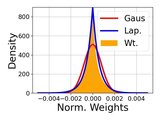
must be protected to maintain the performance [47]; and (2) this inequality (kw(l) k1 ≥ kŵ(l) k1 )
is necessary to apply the iterative compression algorithm based on successive refinement (to be
discussed in Section 5).
In the next section, we develop a NN compression algorithm merging (i) our theoretical findings in
Lemma 1 for optimality and (ii) successive refinement property for practicality.

5     Successive Refinement for Pruning (SuRP)
Rate-distortion theory, although, gives the limit of lossy compression and suggests that pruning
must be a part of a good compression algorithm, does not explicitly give the optimal compression
algorithm. In theory, a compression algorithm could be designed by letting the encoder pick the
closest codeword from a random codebook generated according to the marginal distribution of V in
Lemma 1, as suggested by Shannon [87]. However, such a compressor would not be practical due to
the size of the randomly generated codebook |C| = 2nR(D) (exponential in n – number of weights in
our case). While designing practical compression algorithms without sacrificing the optimality is a
fundamental dilemma in data compression, recent studies have shown that it is possible to design
theoretically optimal schemes with low complexity for certain source distributions. In particular, for
a successively refinable source, an optimal compression algorithm can also be practical [76]. We
exploit this idea for the Laplacian source and develop a practical iterative compression algorithm that
is rate-distortion theoretically optimal. We call it Successive Refinement for Pruning (SuRP) since it
also outputs a sparse model, which can be viewed as a pruned model (although we do not explicitly
prune the model). We first present the successive refinement scheme for Laplacian source that shows
the core idea to achieve lower complexity, but still impractical. We then push further to provide the
practical algorithm and prove the optimality in a rate-distortion theoretic sense.

5.1   Successive Refinement with Randomly Generated Codebooks

Instead of a successive refinement scheme with two decoders as described in Section 3, we consider
the successive refinement problem with L decoders. Let λ = λ1 < · · · < λL where Dt = 1/λt+1 is
a target distortion at the t-th decoder. This is because the error term at iteration t has a Laplacian
distribution with parameter λt+1 = 1/Dt in an optimal compression scheme (see Lemma 1). We
begin by setting U(1) = un . At t-th iteration, the encoder finds V(t) that minimizes the distance
between d(U(t) , V(t) ) from a codebook C (t) , then computes U(t+1) = U(t) − V(t) . More precisely,
the t-th codebook consists of 2nR/L codewords generated by the marginal distribution in Lemma 1:
                                      λ2                    λ2

                                                                    λt
                         fV(t) (v) = 2 t · δ(v) + 1 − 2 t         · e−λt |v|                       (6)
                                     λt+1                  λt+1      2

Since U(t+1) is also an i.i.d. Laplacian random sequence with parameter λt+1 = 1/Dt from the
conditional probability in Lemma 1, the encoder can keep applying the same steps for Laplacian
sources at each iteration. In summary, for 1 ≤ t ≤ L − 1, the information-theoretic successive
refinement encoder performs the following steps iteratively: (1) find V(t) ∈ C (t) that minimizes
d(U(t) , V(t) ); and (2) update U as U(t+1) = U(t) − V(t) . The decoder, on the other hand,
                     Pt
reconstructs Û(t) = τ =1 V(τ ) at iteration t. This scheme has a complexity of L · 2nR/L (the total
size of the codebooks in L iterations), which is lower than the naive random coding strategy (2nR at
once). At the same time, it still achieves the rate-distortion limit, i.e., does not sacrifice the optimality,
thanks to successive refinability of Laplacian source. However, the complexity is still exponential in
n, which is impractical. We fix this in the next section.

5.2   SuRP Algorithm

We saw in Section 5.1 that the information-theoretic approach is rate-distortion theoretic optimal
with lower complexity due to successive refinability, but still impractical with the exponential size
of codebooks. In this section, we develop a new algorithm SuRP, that enjoys both practicality
and optimality. Concretely, SuRP does not require a random codebook or a search for the nearest
codeword V(t) from U(t) at each iteration, yet still rate-distortion theoretic optimal. With the same
initialization U(1) = un and λ1 = λ, new iterative coding scheme for 1 ≤ t ≤ L − 1 is as follows:

                                                      6
(t)                 (t)
      1. Find index i and j such that Ui ≥ λ1t log 2β   n
                                                          and Uj ≤ − λ1t log 2βn
                                                                                  . If there are more
         than one such indices, pick an index i (or j) randomly. Encode (i, j) as mt .
                                                                        (t)       1          n          (t)
      2. Let V(t) be an n-dimensional all-zero vector except Vi               =   λt   log   2β   and Vj      =
                   n
         − λ1t log 2β .
      3. Let U(t+1) = U(t) − V(t) .
                          n
      4. Set λt+1 =   n−2 log   n    · λt .
                                2β

Here, β > 1 is a tunable parameter. Similar to the algorithm in Section 5.1, the reconstruction at t-th
                           Pt
iteration would be Û(t) = τ =1 V(τ ) . We give the pseudocode for SuRP in Appendix D.
                                                                                                              n
                                                                                                    n−2 log
This coding scheme is equivalent to the original scheme in Section 5.1, where λλt+1    t
                                                                                         =       n
                                                                                                    2β

for 1 ≤ t ≤ L − 1 except the fact that the encoder does not do a search over a randomly generated
codebook with exponential size, i.e., SuRP is practical. However, there is still an implicit codebook
C (t) at every iteration t, which consists of n-dimensional all-zero vectors except for two nonzero
                         1       n
elements of values ± λt−1    log 2β . The size of this codebook is n(n − 1) (not exponential anymore).
Since these implicit codebooks are not directly generated from the optimal marginal distribution in
Lemma 1, it is not obvious that SuRP is rate-distortion theoretic optimal. However, we prove in
Section 5.3 that it is rate-distortion theoretic optimal under certain criteria. We highlight that our
scheme can be viewed as a bottom-up approach, in that sparsity in the reconstructed weights starts
from 100% at the first iteration and it decreases as the decoder receives new indices from the encoder
(see Figure 2-right). Similarly, from the same figure, accuracy increases through the iterations.
                                                                        (t)      1       n              (t)
As a practical issue, when there is no index i or j such that Ui ≥ λt−1             log 2β   or Uj ≤
    1         n
− λt−1 log 2β , the encoder re-estimates λ and sends a refreshed value to the decoder. However,
this is a rare situation in our experiments (20 refreshments in 20M iterations) and hence has a negli-
gible effect on the overall optimality. In fact, we control the probability of this undesired situation
(when there is no index to send) with the tunable parameter β. More precisely, the probability that all
Laplacian random variables are smaller than λ1 log 2β n
                                                         in magnitude (i.e., no index i or j found) is

                      1       n                 1      n
    Pr max Xi < log              or min Xi > − log                                                   (7)
                      λ      2β                 λ     2β
                                                                               n
                          1      n                      1      n               1 2β
     ≤ Pr max Xi < log                + Pr min Xi > − log          =2 1−                ≈ 2e−β . (8)
                          λ     2β                      λ     2β               2 n

We set β = log n to bound the probability in Eq. 8 by n2 , which converges to zero as n increases.
Remark 1. From the extreme value theory, it is known that the maximum of n Laplacian random
variables concentrates near λ1 log n2 , which is the case of β = 1. Thus, one iteration of SuRP can
be viewed as finding a near-maximum (and minimum) element. From this perspective, magnitude
pruning can be viewed as a special case of SuRP.
Remark 2. SuRP guarantees kU(t) k1 ≥ kV(t) k1 for all t. This implies that the magnitude of
weights in w is always larger than the magnitude of weights in ŵ. From Theorem 1, we can say that
the `1 weight distortion of SuRP algorithm is an upper bound to the NN model’s output perturbation.

5.3   Zero-Rate Optimality of SuRP

In this section, we prove that SuRP is a zero-rate optimal compression algorithm. Given that SuRP
uses an implicit codebook of size n(n − 1) at each iteration, the rate is found as Rn = log n(n−1)
                                                                                             n     . We
note that Rn gets arbitrarily close to zero as n increases. Moreover, the decrement in the distortion at
                                   2
each iteration is given as Dn = nλ    log 2βnn , where βn = β as before. We start with the definition of
zero-rate optimality, which states that a sub-linear number of bits (in our case log n(n − 1) nats) is
being used optimally in the rate-distortion theoretic sense.
Definition 1 (Zero-rate optimality). A scheme with rate Rn , distortion decrement Dn , and distortion-
rate function D(·), is zero-rate optimal if limn→∞ Rn = 0 and limn→∞ D             0
                                                                           Rn = D (0).
                                                                             n

                                                    7
This implies that a zero-rate optimal scheme achieves the “slope” of the distortion-rate function at
zero rate R = 0. In the case of Laplacian source, this slope is D0 (0) = − λ1 since the distortion-rate
function is D(R) = λ1 e−R , which can be derived from the rate-distortion function in Lemma 1.
Finally, the following theorem states that a single iteration of SuRP is zero-rate optimal.
                                                                            log 2βn
Theorem 2. An iteration of SuRP is zero-rate optimal if limn→∞            log n(n−1)    = 0 holds.

                                                  log n(n−1)               2          n
Proof. In an iteration of SuRP, where Rn =             n       and Dn =   nλ   log   2βn ,   we have
                                 2      n
                   Dn      λ log 2βn     1    log n2     1 2 log 2βn
                      =−              =−               +               .                               (9)
                   Rn    log n(n − 1)    λ log n(n − 1) λ log n(n − 1)
              log 2βn                            Dn
If limn→∞   log n(n−1)   = 0, it is clear that   Rn   converges to D0 (0) = − λ1 as n increases. Therefore,
                                                                      log 2βn
SuRP is zero-rate optimal under the condition that limn→∞           log n(n−1)   = 0.

In Section 5.2, we choose βn = log n to keep the probability in Eq. 8 small. With this choice of βn ,
limn→∞ loglog  2βn
             n(n−1) = 0 holds. Therefore, from Theorem 2, our implementation of SuRP is indeed
zero-rate optimal.
Remark 3. In pure information-theoretic compression setting (main concern is not NN compression),
similar zero-rate optimal schemes were proposed [75, 93] for Gaussian source under mean squared
error, which is also successively refinable. They iteratively applied zero-rate optimal schemes and
further achieved the rate-distortion limit using a special property of Gaussian random variables.

6   Experiments
In this section, we empirically investigate (1) the performance of SuRP compared to other recent
pruning strategies in terms of accuracy-sparsity tradeoff and (2) improvements in the communication
efficiency of federated learning when gradients are compressed with SuRP. We emphasize that the
main contribution of our paper is to bridge the gap between data compression and NN compression
through a rate-distortion theoretic analysis of NN compression problem. SuRP is designed solely
to show that an algorithm derived with an information-theoretic approach indeed outputs a pruned
model, as suggested by the rate-distortion theory. This also provides theoretical support for the recent
success of pruning strategies.
For ease of implementation, instead of reconstructing two weights larger than λ1 log 2βn
                                                                                          in magnitude
                                                         1     n
at each iteration, we reconstruct one weight larger than λ log β . This is equivalent to the algorithm
described in Section 5, and the zero-rate optimality still holds (see AppendixD for details). We
present experimental results averaged over 3-5 runs (see Appendix I for complete results).
We consider three image datasets: CIFAR-10 [53] and ImageNet [17] for NN compression and
MNIST [56] for federated learning experiments. For MNIST, we use LeNet-5-Caffe. For CIFAR-10,
we use two architectures: ResNet-20 [39] and VGG-16 [88]. For ImageNet, we use ResNet-50
[39, 79]. We give additional details on model architectures and hyperparameters in Appendix H.
NN Compression/Pruning: In Table 1 and Figure 2-left, we compare our scheme with the recent
pruning papers. We apply iterative pruning, meaning that we apply SuRP in repeating cycles (see
Appendix I for details). As baselines, we consider Global [73], Uniform [109], and Adaptive [27]
pruning techniques and LAMP [58]. Additionally, we include comparisons to recent works on weight
rewinding and dynamic sparsity, in particular SNIP [59], DSR [74], SNFS [18], and RiGL [22].
We present the performance of pruned ResNet-50 on ImageNet in Figure 2-left, and VGG-16 and
ResNet-20 architectures on CIFAR-10 in Table 1. As can be seen from Table 1, SuRP outperforms
prior work in all sparsity levels. From Figure 2-left, SuRP and Adaptive pruning [28] perform
similarly (with ±0.06% difference in the accuracy), and they both outperform other baselines.
We emphasize that our algorithm SuRP has an additional advantage in optimizing the bit rate of the
model thanks to the rate-distortion theoretic basis of our approach. In particular, the decoder has only
access to a list of indices, and these indices represent the whole (compressed) model – more efficient
than describing the precise values of surviving weights. However, our current implementation does

                                                        8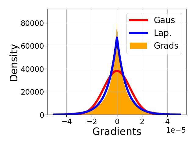
Pruning Ratio:        80%       90%
    Adaptive [27]        75.60      73.90
    SNIP [59]            72.00      67.20
    DSR [74]             73.30      71.60
    SNFS [18]            74.90      72.90
    RiGL [22]            74.60      72.00
    SuRP (ours)          75.54      73.93

Figure 2: (left) Accuracy of ResNet-50 on ImageNet. Results are averaged over three runs. (right)
Sparsity and accuracy of the reconstructed ResNet-50 on ImageNet during one cycle of SuRP.
Iterations correspond to the iterations running inside SuRP.

not exploit this efficiency to the full extent due to retraining steps after each pruning iteration. Like
many, we will also look for ways to prune (compress in general) NN models without a retraining step
afterward. That way, SuRP can be improved to provide a better accuracy-bit rate tradeoff, together
with the already demonstrated superior sparsity-accuracy tradeoff. We give more details on this and
share experimental results in Appendix F and I. Finally, to give an idea about the bit rate efficiency of
SuRP, we apply it for compressing gradients in a federated learning setting. Since the compressed
gradients are not exposed to fine-tuning (like retraining in pruning), SuRP provides a substantial
improvement on the bit rate compared to prior work. We elaborate more on this in the next paragraph.

                Pruning Ratio: 93.12% 95.60% 97.19% 98.20% 98.85% 99.26% 99.53% 99.70% 99.81% 99.88%
                 Global [73]    91.30   90.80   89.28   85.55   81.56   54.58   41.91   31.93   21.87   11.72
                Uniform [109]   91.47   90.78   88.61   84.17   55.68   38.51   26.41   16.75   11.58    9.95
                Adaptive [27]   91.54   91.20   90.16   89.44   87.85   86.53   84.84   82.41   74.54   24.46
    VGG-16
                 RiGL [22]      92.34   91.99   91.66   91.15   90.55   89.51   88.21   86.73   84.85   81.50
                 LAMP [58]      92.24   92.06   91.71   91.66   91.07   90.49   89.64   88.75   87.07   84.90
                SuRP (ours)     92.55   92.13   91.95   91.72   91.21   90.73   90.65   89.70   87.28   85.04
                Pruning Ratio: 79.03% 86.58% 91.41% 94.50% 96.48% 97.75% 98.56% 99.08% 99.41% 99.62%
                 Global [73]    87.48   86.97   86.29   85.02   83.15   80.52   76.28   70.69   47.47   12.02
                Uniform [109]   87.24   86.70   86.09   84.53   82.05   77.19   64.24   47.97   20.45   13.35
                Adaptive [27]   87.30   87.00   86.27   85.00   83.23   80.40   76.40   69.31   52.06   20.19
    ResNet-20
                  RiGL [22]     87.63   87.49   86.83   85.84   84.08   81.76   78.70   74.40   66.42   50.90
                 LAMP [58]      87.54   87.12   86.56   85.64   84.18   81.56   78.63   74.20   67.01   51.24
                 SuRP (ours)    91.37   90.44   89.00   88.87   87.05   83.98   79.00   74.86   70.64   54.22

 Table 1: Accuracy of VGG-16 and ResNet-20 on CIFAR-10. Results are averaged over five runs.

Compression for Federated Learning (FL): FL is a distributed training setting where edge devices
are responsible for doing local training and sending local gradients to a central server [50]. Given
the resource limitations of edge devices, gradient communication is a significant bottleneck in FL,
and gradient compression is crucial [51]. We show in Appendix G that Laplacian distribution is a
good fit for NN gradients. Therefore, SuRP is applicable to this problem as well. Our preliminary
experiments with LeNet-5-Caffe on MNIST compare SuRP with DGC [63] and rTop-k [4]. We
compute the communication budget for prior work by assuming a naive encoding with k(log n + 32)
bits (n is the model size) since no other method is provided. With the same sparsity ratio 99.9%, DGC
achieves 98.5% accuracy with 2.05KB of budget, rTop-k achieves 99.1% accuracy with 2.05KB of
budget, and SuRP achieves 99.1% accuracy with 218B of budget. Thus, SuRP provides 10× times
improvement in the gradients’ compression rate while achieving the same accuracy as rTop-k.

7      Discussion and Conclusion

In this work, we connected two lines of research, namely, data compression and NN compression.
In particular, we explained the compressibility of NN models via rate-distortion theory. Although
our initial goal was to understand the theoretical tradeoff between the compression ratio and output
perturbation, we found out that the rate-distortion theoretic formulation of the problem also introduces
a theoretical foundation for pruning. Guided by this, we developed a NN compression algorithm that
outputs a pruned model and outperforms prior work on CIFAR-10 and ImageNet datasets.

                                                         9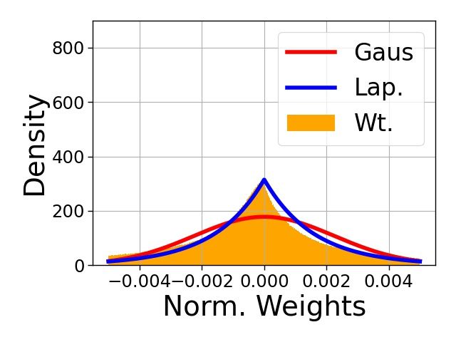
Limitations: One limitation of the proposed approach is i.i.d. source assumption. While previous
score-based pruning approaches make the same assumption implicitly, empirical results indicate that
NN weights are correlated, hence not independent. In future work, we plan to formalize the problem
without i.i.d. assumption while also hypothesizing about the source distribution more rigorously.
Societal Impact: When we evaluated our strategy, we only considered accuracy as a metric.
However, compression might have a negative impact on other properties of the model as well, such
as fairness, as pointed out in a recent work [41]. Like many NN compression works, our distortion
function does not address the potential disproportionate effects of compression on different subgroups
of data. We agree that this is an issue that must attract more attention from the research community.

8     Acknowledgement
This work was supported in part by a Sony Stanford Graduate Fellowship.

References
    [1] A. F. Aji and K. Heafield. Sparse communication for distributed gradient descent. arXiv
        preprint arXiv:1704.05021, 2017.
    [2] J. Ballé, V. Laparra, and E. P. Simoncelli. End-to-end optimized image compression. arXiv
        preprint arXiv:1611.01704, 2016.
    [3] R. Banner, I. Hubara, E. Hoffer, and D. Soudry. Scalable methods for 8-bit training of neural
        networks. In Advances in neural information processing systems, pages 5145–5153, 2018.
    [4] L. P. Barnes, H. A. Inan, B. Isik, and A. Ozgur. rtop-k: A statistical estimation approach to
        distributed sgd. arXiv preprint arXiv:2005.10761, 2020.
    [5] T. Berger. Rate-distortion theory. Wiley Encyclopedia of Telecommunications, 2003.
    [6] D. Blalock, J. J. G. Ortiz, J. Frankle, and J. Guttag. What is the state of neural network
        pruning? arXiv preprint arXiv:2003.03033, 2020.
    [7] C. Bucilua, R. Caruana, and A. Niculescu-Mizil. Model compression. In Proceedings of the
        12th ACM SIGKDD International Conference on Knowledge Discovery and Data Mining,
        KDD ’06, page 535–541, New York, NY, USA, 2006. Association for Computing Machinery.
        ISBN 1595933395. doi: 10.1145/1150402.1150464. URL https://doi.org/10.1145/
        1150402.1150464.
    [8] M. A. Carreira-Perpinan and Y. Idelbayev. “learning-compression” algorithms for neural net
        pruning. In Proceedings of the IEEE Conference on Computer Vision and Pattern Recognition,
        pages 8532–8541, 2018.
    [9] G. Castellano, A. M. Fanelli, and M. Pelillo. An iterative pruning algorithm for feedforward
        neural networks. IEEE transactions on Neural networks, 8(3):519–531, 1997.
 [10] T. Chen, Z. Zhang, S. Liu, S. Chang, and Z. Wang. Long live the lottery: The existence of
      winning tickets in lifelong learning. In International Conference on Learning Representations,
      2021a. URL https://openreview. net/forum, 2021.
 [11] Y. Cheng, D. Wang, P. Zhou, and T. Zhang. Model compression and acceleration for deep
      neural networks: The principles, progress, and challenges. IEEE Signal Processing Magazine,
      35(1):126–136, 2018.
 [12] Y. Choi, M. El-Khamy, and J. Lee. Universal deep neural network compression. IEEE Journal
      of Selected Topics in Signal Processing, 2020.
 [13] T. M. Cover and J. A. Thomas. Elements of Information Theory (Wiley Series in Telecommuni-
      cations and Signal Processing). Wiley-Interscience, USA, 2006. ISBN 0471241954.
 [14] Y. L. Cun, J. S. Denker, and S. A. Solla. Optimal Brain Damage, page 598–605. Morgan
      Kaufmann Publishers Inc., San Francisco, CA, USA, 1990. ISBN 1558601007.

                                                 10
[15] B. Dai, C. Zhu, B. Guo, and D. Wipf. Compressing neural networks using the variational
information bottleneck. In J. Dy and A. Krause, editors, Proceedings of the 35th International
Conference on Machine Learning, volume 80 of Proceedings of Machine Learning Research,
pages 1135–1144. PMLR, 10–15 Jul 2018. URL http://proceedings.mlr.press/v80/
dai18d.html.
[16] J. Dean, G. Corrado, R. Monga, K. Chen, M. Devin, M. Mao, M. Ranzato, A. Senior, P. Tucker,
K. Yang, et al. Large scale distributed deep networks. In Advances in neural information
processing systems, pages 1223–1231, 2012.
[17] J. Deng, W. Dong, R. Socher, L.-J. Li, K. Li, and L. Fei-Fei. ImageNet: A Large-Scale
Hierarchical Image Database. In CVPR09, 2009.
[18] T. Dettmers and L. Zettlemoyer. Sparse networks from scratch: Faster training without losing
performance. arXiv preprint arXiv:1907.04840, 2019.
[19] E. Elsen, M. Dukhan, T. Gale, and K. Simonyan. Fast sparse convnets. In Proceedings of the
IEEE/CVF conference on computer vision and pattern recognition, pages 14629–14638, 2020.
[20] A. P. Engelbrecht. A new pruning heuristic based on variance analysis of sensitivity information.
IEEE transactions on Neural Networks, 12(6):1386–1399, 2001.
[21] W. H. Equitz and T. M. Cover. Successive refinement of information. IEEE Transactions on
Information Theory, 37(2):269–275, 1991.
[22] U. Evci, T. Gale, J. Menick, P. S. Castro, and E. Elsen. Rigging the lottery: Making all tickets
winners. In International Conference on Machine Learning, pages 2943–2952. PMLR, 2020.
[23] M. Federici, K. Ullrich, and M. Welling. Improved bayesian compression. arXiv preprint
arXiv:1711.06494, 2017.
[24] J. Frankle and M. Carbin. The lottery ticket hypothesis: Finding sparse, trainable neural
networks. International Conference on Learning Representations (ICLR), 2019.
[25] J. Frankle, G. K. Dziugaite, D. Roy, and M. Carbin. Linear mode connectivity and the lottery
ticket hypothesis. In International Conference on Machine Learning, pages 3259–3269. PMLR,
2020.
[26] J. Frankle, G. K. Dziugaite, D. M. Roy, and M. Carbin. Pruning neural networks at initialization:
Why are we missing the mark? arXiv preprint arXiv:2009.08576, 2020.
[27] T. Gale, E. Elsen, and S. Hooker. The state of sparsity in deep neural networks. arXiv preprint
arXiv:1902.09574, 2019.
[28] T. Gale, M. Zaharia, C. Young, and E. Elsen. Sparse gpu kernels for deep learning. arXiv
preprint arXiv:2006.10901, 2020.
[29] R. Gallager and D. Van Voorhis. Optimal source codes for geometrically distributed integer
alphabets (corresp.). IEEE Transactions on Information theory, 21(2):228–230, 1975.
[30] W. Gao, Y.-H. Liu, C. Wang, and S. Oh. Rate distortion for model compression: From theory
to practice. In International Conference on Machine Learning, pages 2102–2111. PMLR,
2019.
[31] S. Golomb. Run-length encodings (corresp.). IEEE transactions on information theory, 12(3):
399–401, 1966.
[32] J. Gou, B. Yu, S. J. Maybank, and D. Tao. Knowledge distillation: A survey. International
Journal of Computer Vision, pages 1–31, 2021.
[33] P. D. Grünwald and A. Grunwald. The minimum description length principle. MIT press,
2007.
[34] Y. Guo, A. Yao, and Y. Chen. Dynamic network surgery for efficient dnns. In Advances in
neural information processing systems, pages 1379–1387, 2016.
11[35] S. Han, J. Pool, J. Tran, and W. Dally. Learning both weights and connections for efficient
neural network. In Advances in neural information processing systems, pages 1135–1143,
2015.
[36] S. Han, H. Mao, and W. J. Dally. Deep compression: Compressing deep neural networks
with pruning, trained quantization and huffman coding. International Conference on Learning
Representations (ICLR), 2016.
[37] B. Hassibi, D. G. Stork, G. Wolff, and T. Watanabe. Optimal brain surgeon: Extensions and
performance comparisons. In Proceedings of the 6th International Conference on Neural
Information Processing Systems, NIPS’93, page 263–270, San Francisco, CA, USA, 1993.
[38] M. Havasi, R. Peharz, and J. M. Hernández-Lobato. Minimal random code learning: Getting
bits back from compressed model parameters. In International Conference on Learning
Representations (ICLR), 2019.
[39] K. He, X. Zhang, S. Ren, and J. Sun. Deep residual learning for image recognition. In
Proceedings of the IEEE conference on computer vision and pattern recognition, pages 770–
778, 2016.
[40] G. Hinton, O. Vinyals, and J. Dean. Distilling the knowledge in a neural network. In NIPS
Deep Learning and Representation Learning Workshop, 2015. URL http://arxiv.org/
abs/1503.02531.
[41] S. Hooker, N. Moorosi, G. Clark, S. Bengio, and E. Denton. Characterising bias in compressed
models. arXiv preprint arXiv:2010.03058, 2020.
[42] D. A. Huffman. A method for the construction of minimum-redundancy codes. Proceedings
of the IRE, 40(9):1098–1101, 1952.
[43] Y. Idelbayev and M. A. Carreira-Perpinan. Low-rank compression of neural nets: Learning
the rank of each layer. In Proceedings of the IEEE/CVF Conference on Computer Vision and
Pattern Recognition (CVPR), June 2020.
[44] Y. Idelbayev and M. A. Carreira-Perpinan. Neural network compression via additive combina-
tion of reshaped, low-rank matrices. In 2021 Data Compression Conference (DCC), pages
243–252, 2021. doi: 10.1109/DCC50243.2021.00032.
[45] Y. Idelbayev, P. Molchanov, M. Shen, H. Yin, M. A. Carreira-Perpinan, and J. M. Alvarez.
Optimal quantization using scaled codebook. In Proc. of the 2021 IEEE Computer Society
Conf. Computer Vision and Pattern Recognition (CVPR’21), Virtual, 2021.
[46] Y. Ioannou, D. Robertson, J. Shotton, R. Cipolla, and A. Criminisi. Training cnns with
low-rank filters for efficient image classification. arXiv preprint arXiv:1511.06744, 2015.
[47] B. Isik, K. Choi, X. Zheng, T. Weissman, S. Ermon, H. S. P. Wong, and A. Alaghi. Neural
network compression for noisy storage devices. arXiv preprint arXiv:2102.07725, 2021.
[48] B. Jacob, S. Kligys, B. Chen, M. Zhu, M. Tang, A. Howard, H. Adam, and D. Kalenichenko.
Quantization and training of neural networks for efficient integer-arithmetic-only inference.
In Proceedings of the IEEE Conference on Computer Vision and Pattern Recognition, pages
2704–2713, 2018.
[49] S. Jung, C. Son, S. Lee, J. Son, J.-J. Han, Y. Kwak, S. J. Hwang, and C. Choi. Learning to
quantize deep networks by optimizing quantization intervals with task loss. In Proceedings of
the IEEE/CVF Conference on Computer Vision and Pattern Recognition, pages 4350–4359,
2019.
[50] P. Kairouz, H. B. McMahan, B. Avent, A. Bellet, M. Bennis, A. N. Bhagoji, K. Bonawitz,
Z. Charles, G. Cormode, R. Cummings, et al. Advances and open problems in federated
learning. arXiv preprint arXiv:1912.04977, 2019.
[51] J. Konečný, H. B. McMahan, F. X. Yu, P. Richtarik, A. T. Suresh, and D. Bacon. Federated
learning: Strategies for improving communication efficiency. In NIPS Workshop on Private
Multi-Party Machine Learning, 2016.
12[52] V. N. Koshelev. Hierarchical coding of discrete sources. Problemy peredachi informatsii, 16
(3):31–49, 1980.
[53] A. Krizhevsky, G. Hinton, et al. Learning multiple layers of features from tiny images. 2009.
[54] A. Kusupati, V. Ramanujan, R. Somani, M. Wortsman, P. Jain, S. Kakade, and A. Farhadi.
Soft threshold weight reparameterization for learnable sparsity. In International Conference
on Machine Learning, pages 5544–5555. PMLR, 2020.
[55] Y. LeCun, L. Bottou, Y. Bengio, and P. Haffner. Gradient-based learning applied to document
recognition. Proceedings of the IEEE, 86(11):2278–2324, 1998.
[56] Y. LeCun, C. Cortes, and C. Burges. Mnist handwritten digit database, 2010.
[57] Y. LeCun, Y. Bengio, and G. Hinton. Deep learning. nature, 521(7553):436–444, 2015.
[58] J. Lee, S. Park, S. Mo, S. Ahn, and J. Shin. Layer-adaptive sparsity for the magnitude-based
pruning. International Conference on Learning Representations, 2021.
[59] N. Lee, T. Ajanthan, and P. H. Torr. Snip: Single-shot network pruning based on connection
sensitivity. arXiv preprint arXiv:1810.02340, 2018.
[60] F. Li, B. Zhang, and B. Liu. Ternary weight networks. arXiv preprint arXiv:1605.04711, 2016.
[61] J. Lin, Y. Rao, J. Lu, and J. Zhou. Runtime neural pruning. In Proceedings of the 31st
International Conference on Neural Information Processing Systems, pages 2178–2188, 2017.
[62] S. Lin, R. Ji, C. Yan, B. Zhang, L. Cao, Q. Ye, F. Huang, and D. Doermann. Towards optimal
structured cnn pruning via generative adversarial learning. In Proceedings of the IEEE/CVF
Conference on Computer Vision and Pattern Recognition, pages 2790–2799, 2019.
[63] Y. Lin, S. Han, H. Mao, Y. Wang, and W. J. Dally. Deep gradient compression: Reducing
the communication bandwidth for distributed training. International Conference on Learning
Representations (ICLR), 2017.
[64] Z. Liu, M. Sun, T. Zhou, G. Huang, and T. Darrell. Rethinking the value of network pruning.
arXiv preprint arXiv:1810.05270, 2018.
[65] Z. Liu, J. Xu, X. Peng, and R. Xiong. Frequency-domain dynamic pruning for convolutional
neural networks. In Proceedings of the 32nd International Conference on Neural Information
Processing Systems, pages 1051–1061, 2018.
[66] Z. Liu, H. Mu, X. Zhang, Z. Guo, X. Yang, K.-T. Cheng, and J. Sun. Metapruning: Meta
learning for automatic neural network channel pruning. In Proceedings of the IEEE/CVF
International Conference on Computer Vision, pages 3296–3305, 2019.
[67] C. Louizos, K. Ullrich, and M. Welling. Bayesian compression for deep learning. arXiv
preprint arXiv:1705.08665, 2017.
[68] C. Louizos, M. Welling, and D. P. Kingma. Learning sparse neural networks through l_0
regularization. arXiv preprint arXiv:1712.01312, 2017.
[69] H. B. McMahan, E. Moore, D. Ramage, S. Hampson, and B. A. y Arcas. Communication-
efficient learning of deep networks from decentralized data. In AISTATS, 2017.
[70] D. C. Mocanu, E. Mocanu, P. Stone, P. H. Nguyen, M. Gibescu, and A. Liotta. Scalable
training of artificial neural networks with adaptive sparse connectivity inspired by network
science. Nature communications, 9(1):1–12, 2018.
[71] D. Molchanov, A. Ashukha, and D. Vetrov. Variational dropout sparsifies deep neural networks.
In International Conference on Machine Learning, pages 2498–2507. PMLR, 2017.
[72] P. Molchanov, S. Tyree, T. Karras, T. Aila, and J. Kautz. Pruning convolutional neural networks
for resource efficient inference. arXiv preprint arXiv:1611.06440, 2016.
13[73] A. S. Morcos, H. Yu, M. Paganini, and Y. Tian. One ticket to win them all: generalizing lottery
ticket initializations across datasets and optimizers. arXiv preprint arXiv:1906.02773, 2019.
[74] H. Mostafa and X. Wang. Parameter efficient training of deep convolutional neural networks
by dynamic sparse reparameterization. In International Conference on Machine Learning,
pages 4646–4655. PMLR, 2019.
[75] A. No and T. Weissman. Rateless lossy compression via the extremes. IEEE transactions on
information theory, 62(10):5484–5495, 2016.
[76] A. No, A. Ingber, and T. Weissman. Strong successive refinability and rate-distortion-
complexity tradeoff. IEEE Transactions on Information Theory, 62(6):3618–3635, 2016.
[77] D. Oktay, J. Ballé, S. Singh, and A. Shrivastava. Scalable model compression by entropy
penalized reparameterization. In International Conference on Learning Representations
(ICLR), 2019.
[78] S. Park, J. Lee, S. Mo, and J. Shin. Lookahead: A far-sighted alternative of magnitude-based
pruning. International Conference on Learning Representations (ICLR), 2020.
[79] A. Paszke, S. Gross, F. Massa, A. Lerer, J. Bradbury, G. Chanan, T. Killeen, Z. Lin,
N. Gimelshein, L. Antiga, A. Desmaison, A. Kopf, E. Yang, Z. DeVito, M. Raison, A. Te-
jani, S. Chilamkurthy, B. Steiner, L. Fang, J. Bai, and S. Chintala. Pytorch: An imperative
style, high-performance deep learning library. In H. Wallach, H. Larochelle, A. Beygelzimer,
F. d'Alché-Buc, E. Fox, and R. Garnett, editors, Advances in Neural Information Processing
Systems 32, pages 8024–8035. Curran Associates, Inc., 2019.
[80] H. Peng, J. Wu, S. Chen, and J. Huang. Collaborative channel pruning for deep networks. In
International Conference on Machine Learning, pages 5113–5122. PMLR, 2019.
[81] A. Polino, R. Pascanu, and D. Alistarh. Model compression via distillation and quantization.
arXiv preprint arXiv:1802.05668, 2018.
[82] A. Renda, J. Frankle, and M. Carbin. Comparing fine-tuning and rewinding in neural network
pruning. In International Conference on Learning Representations, 2020.
[83] T. N. Sainath, B. Kingsbury, V. Sindhwani, E. Arisoy, and B. Ramabhadran. Low-rank matrix
factorization for deep neural network training with high-dimensional output targets. In 2013
IEEE international conference on acoustics, speech and signal processing, pages 6655–6659.
IEEE, 2013.
[84] D. Salomon. Data compression: the complete reference. Springer Science & Business Media,
2004.
[85] V. Sehwag, S. Wang, P. Mittal, and S. Jana. Hydra: Pruning adversarially robust neural
networks. Advances in Neural Information Processing Systems (NeurIPS), 7, 2020.
[86] C. E. Shannon. Coding theorems for a discrete source with a fidelity criterion. IRE Nat. Conv.
Rec, 4(142-163):1, 1959.
[87] C. E. Shannon. A mathematical theory of communication. ACM SIGMOBILE mobile comput-
ing and communications review, 5(1):3–55, 2001.
[88] K. Simonyan and A. Zisserman. Very deep convolutional networks for large-scale image
recognition. arXiv preprint arXiv:1409.1556, 2014.
[89] S. P. Singh and D. Alistarh. Woodfisher: Efficient second-order approximations for model
compression. arXiv preprint arXiv:2004.14340, 2020.
[90] S. Srinivas and R. V. Babu. Data-free parameter pruning for deep neural networks. arXiv
preprint arXiv:1507.06149, 2015.
[91] P. Stock, A. Fan, B. Graham, E. Grave, R. Gribonval, H. Jegou, and A. Joulin. Training with
quantization noise for extreme model compression. In International Conference on Learning
Representations, 2021. URL https://openreview.net/forum?id=dV19Yyi1fS3.
14[92] K. Ullrich, E. Meeds, and M. Welling. Soft weight-sharing for neural network compression.
arXiv preprint arXiv:1702.04008, 2017.
[93] R. Venkataramanan, T. Sarkar, and S. Tatikonda. Lossy compression via sparse linear regres-
sion: Computationally efficient encoding and decoding. IEEE transactions on information
theory, 60(6):3265–3278, 2014.
[94] S. Verdu. The exponential distribution in information theory. Problemy peredachi informatsii,
32(1):100–111, 1996.
[95] H. Wang, S. Sievert, S. Liu, Z. B. Charles, D. S. Papailiopoulos, and S. Wright. Atomo:
Communication-efficient learning via atomic sparsification. In NeurIPS, 2018.
[96] J. Wang, W. Bao, L. Sun, X. Zhu, B. Cao, and S. Y. Philip. Private model compression via
knowledge distillation. In Proceedings of the AAAI Conference on Artificial Intelligence,
volume 33, pages 1190–1197, 2019.
[97] K. Wang, Z. Liu, Y. Lin, J. Lin, and S. Han. Haq: Hardware-aware automated quantization
with mixed precision. In Proceedings of the IEEE/CVF Conference on Computer Vision and
Pattern Recognition, pages 8612–8620, 2019.
[98] Y. Wang, X. Zhang, L. Xie, J. Zhou, H. Su, B. Zhang, and X. Hu. Pruning from scratch. In
Proceedings of the AAAI Conference on Artificial Intelligence, volume 34, pages 12273–12280,
2020.
[99] J. Wangni, J. Wang, J. Liu, and T. Zhang. Gradient sparsification for communication-efficient
distributed optimization. In S. Bengio, H. Wallach, H. Larochelle, K. Grauman, N. Cesa-
Bianchi, and R. Garnett, editors, Advances in Neural Information Processing Systems 31,
pages 1299–1309. Curran Associates, Inc., 2018.
[100] S. Wiedemann, H. Kirchhoffer, S. Matlage, P. Haase, A. Marban, T. Marinč, D. Neumann,
T. Nguyen, H. Schwarz, T. Wiegand, D. Marpe, and W. Samek. Deepcabac: A universal
compression algorithm for deep neural networks. IEEE Journal of Selected Topics in Signal
Processing, 14(4):700–714, 2020.
[101] P. M. Williams. Bayesian regularization and pruning using a laplace prior. Neural computation,
7(1):117–143, 1995.
[102] X. Xiao, Z. Wang, and S. Rajasekaran. Autoprune: Automatic network pruning by regularizing
auxiliary parameters. Advances in neural information processing systems, 32, 2019.
[103] T.-J. Yang, Y.-H. Chen, and V. Sze. Designing energy-efficient convolutional neural networks
using energy-aware pruning. In Proceedings of the IEEE Conference on Computer Vision and
Pattern Recognition (CVPR), July 2017.
[104] P. Yin, S. Zhang, J. Lyu, S. Osher, Y. Qi, and J. Xin. Binaryrelax: A relaxation approach for
training deep neural networks with quantized weights. SIAM Journal on Imaging Sciences, 11
(4):2205–2223, 2018.
[105] S. I. Young, W. Zhe, D. Taubman, and B. Girod. Transform quantization for cnn compression.
arXiv preprint arXiv:2009.01174, 2020.
[106] R. Yu, A. Li, C.-F. Chen, J.-H. Lai, V. I. Morariu, X. Han, M. Gao, C.-Y. Lin, and L. S. Davis.
Nisp: Pruning networks using neuron importance score propagation. In Proceedings of the
IEEE Conference on Computer Vision and Pattern Recognition, pages 9194–9203, 2018.
[107] C. Zhao, B. Ni, J. Zhang, Q. Zhao, W. Zhang, and Q. Tian. Variational convolutional neural
network pruning. In Proceedings of the IEEE/CVF Conference on Computer Vision and
Pattern Recognition, pages 2780–2789, 2019.
[108] W. Zhe, J. Lin, M. S. Aly, S. Young, V. Chandrasekhar, and B. Girod. Rate-distortion optimized
coding for efficient cnn compression. In 2021 Data Compression Conference (DCC), pages
253–262. IEEE, 2021.
[109] M. Zhu and S. Gupta. To prune, or not to prune: exploring the efficacy of pruning for model
compression. arXiv preprint arXiv:1710.01878, 2017.
15You can also read