Is the Covid equity bubble rational? A machine learning answer - Finance Innovation
←
→
Page content transcription
If your browser does not render page correctly, please read the page content below
Is the Covid equity bubble rational?
                                          A machine learning answer

                        Jean Jacques Ohana 1 Eric Benhamou 2 3 David Saltiel 2 4 Beatrice Guez 2

                           Abstract                                    group of traditional investment managers and in particular
       Is the Covid Equity bubble rational? In 2020,                   whose qualified as value, this excitement is not very under-
       stock prices ballooned with S&P 500 gaining                     standable neither explainable or audible. Current valuations
       16%, and the tech-heavy Nasdaq soaring to 43%,                  are absurd and totally disconnected from the fundamentals
       while fundamentals deteriorated with decreasing                 of the company and the macroeconomic context. In contrast,
       GDP forecasts, shrinking sales and revenues esti-               for the young millennials and in particular the Covid gener-
       mates and higher government deficits. To answer                 ation also referred to as the Robinhood traders, named after
       this fundamental question, with little bias as possi-           the stock exchange platform created in the United States on
       ble, we explore a gradient boosting decision trees              which all (young) Americans who are interested in stock
       (GBDT) approach that enables us to crunch nu-                   markets are, this is completely logic. Stocks can only go
       merous variables and let the data speak. We define              up. For them, there is no need to be interested in macroeco-
       a crisis regime to identify specific downturns in               nomics to invest in the stock market. They just have to ride
       stock markets and normal rising equity markets.                 the wave and in particular the news and jump on stocks that
       We test our approach and report improved accu-                  everyone is looking after. For sure, markets cannot reach
       racy of GBDT over other ML methods. Thanks                      the sky. But at least on the short term, one must concede
       to Shapley values, we are able to identify most                 that markets are still in bull regime. And the real question is
       important features, making this current work in-                not whether this bubble is going to burst but when thanks
       novative and a suitable answer to the justification             to a proper understanding of the rational behind it. If we
       of current equity level.                                        are precisely able to get the logic, we can have a chance to
                                                                       detect when stocks will reverse. Hence the true question is
                                                                       not to say if market are overvalued or not but find the key
1. Introduction                                                        drivers and rational behind current level. To answer this
                                                                       question, we take a machine learning point of view as we
Recent stock market news are filled more than ever with                want to use a large quantity of data and be able to extract
euphoric and frenetic stories about easy and quick money.              information.
Take for instance the Tesla stock. Its market capitalization
is now hovering around $ 850 billion USD, despite a price              The novelty of this approach is to answer an economical
earning over 134 to be compared with the automotive indus-             debate whether equity market current valuation makes sense
try PE of 18 and a market capitalization larger than the sum           using a very modern and scientific approach thanks to ma-
of the next nine largest automotive companies. Likewise,               chine learning that is able to exploit many variables and
bitcoin has gone ballistic reaching 40 000 USD despite its             provides answer without any specific bias. In contrast to
pure virtual status, its implicit connection to criminal crime         statistical approaches that are often geared towards validat-
or fraudulent money and recurrent stories of electronic wal-           ing a human intuition, machine learning can provide new
lets lost or hack. Likewise, unknown companies have been               reasoning and unknown and non linear relationship between
suddenly put on the front stage because of some tweets or              variables and output. In this work, we explore a gradi-
other social media hot news. This has been for instance                ent boosting decision trees (GBDT) approach to provide a
the case of the company Signal that was confused with the              suitable and explainable answer to the rationality of Covid
social media company and whose share exploded despite                  equity bubble.
being non related to the social media Signal app. For a large
                                                                       1.1. Related works
   1
    Homa Capital, France 2 Ai for Alpha, France 3 Lamsade, Paris
Dauphine, France 4 Lisic, ULCO, France. Correspondence to: Jean        Our work can be related to the ever growing theme of using
Jacques Ohana .                                machine learning in financial markets. Indeed, with increas-
                                                                       ing competition and pace in the financial markets, robust
                                                                   1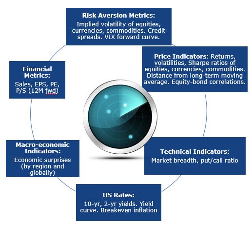
forecasting methods has become a vital subject for asset             of input data types and in particular text inputs. But when
managers. The promise of machine learning algorithms to              it comes to small data set like daily data with properly for-
offer a way to find and model non-linearity in time series           matted data from times series, the real choice of the best
has attracted lot of attention and efforts that can be traced        machine learning is not so obvious.
back as early as the late 2000’s where machine learning
                                                                     Interestingly, Gradient boosting decision trees (GBDT) are
started to pick up. Instead of listing the large amount of
                                                                     almost non-existent in the financial market forecasting liter-
works, we will refer readers to various works that reviewed
                                                                     ature. One can argue that GBDT are well known to suffer
the existing literature in chronological order.
                                                                     from over fitting when tackling regression problems. How-
In 2009, (Atsalakis & Valavanis, 2009) surveyed already              ever, they are the method of choice for classification prob-
more than 100 related published articles using neural and            lems as reported by the machine learning platform Kaggle.
neuro-fuzzy techniques derived and applied to forecast stock         In finance, the only space where GBDT are really cited in
markets, or discussing classifications of financial market           the literature is the credit scoring and retail banking. For
data and forecasting methods. In 2010, (Li & Ma, 2010)               instance, (Brown & Mues, 2012) or (Marceau et al., 2019)
gave a survey on the application of artificial neural networks       reported that GBDT are the best ML method for this specific
in forecasting financial market prices, including exchange           task as they can cope with limited amount of data and very
rates, stock prices, and financial crisis prediction as well         imbalanced classes.
as option pricing. And the stream of machine learning was
                                                                     If we are interested in classifying stock market into two
not only based on neural network but also generic and evo-
                                                                     regimes: a normal rising one and a crisis one, we are pre-
lutionary algorithms as reviewed in (Aguilar-Rivera et al.,
                                                                     cisely facing very imbalanced classes and a binary classi-
2015).
                                                                     fication challenge. In addition, if we are looking at daily
More recently, (Xing et al., 2018) reviewed the application          observations, we have also a machine learning problem with
of cutting-edge NLP techniques for financial forecasting,            limited number of data. This two points can hinder seri-
using text from financial news or twitters. (Rundo et al.,           ously the performance of deep learning algorithms that are
2019) covered the wider topic of usage of machine learning           well known to be data greedy. Hence, our work has con-
techniques, including deep learning, to financial portfolio          sisted in researching whether GBDT can provide a suitable
allocation and optimization systems. (Nti et al., 2019) fo-          method to identify regimes in stock markets. In addition, as
cused on the usage of support vector machine and artificial          a byproduct, GBDT provide explicit rules (even if they can
neural networks to forecast prices and regimes based on              be quite complex) as opposed to deep learning making it an
fundamental and technical analysis. Later on, (Shah et al.,          ideal candidate to investigate regime qualification for stock
2019) discussed some of the challenges and research op-              markets. In this work, we apply our methodology to the US
portunities, including issues for algorithmic trading, back          S&P 500 future. Naturally, this can be easily transposed
testing and live testing on single stocks and more gener-            and extended to other main stock markets like the Nasdaq,
ally prediction in financial market. Finally, (Sezer et al.,         the Eurostoxx, the FTSE, the Nikkei or the MSCI Emerging
2019) reviewed not only deep learning methods but also               future.
other machine learning methods to forecast financial times.
As the hype has been recently mostly on deep learning, it            1.2. Contribution
is not a surprise that most of their reviewed works are on
deep learning. The only work cited that is gradient boosted          Our contributions are threefold:
decision tree is (Krauss et al., 2017)
                                                                        • we specify a valid methodology using GBDT to deter-
In addition, there are works that aim to review the best al-              mine regimes in financial markets, based on a combi-
gorithms for predicting financial markets. With only a few                nation of more than 150 features including financial
exceptions, these papers argue that deep networks outper-                 metrics, macro economics, risk aversion, price and
form traditional machine learning techniques, like support                technical indicators. Not only does this provide a suit-
vector machine or logistic regression. There is however                   able explanation for current equity levels thanks to
the notable exception of (Ballings et al., 2015) that argue               features analysis but it also provides a tool to attempt
that Random Forest is the best algorithm when compared                    for early signals should a turn point in the market come.
with peers like Support Vector Machines, Kernel Factory,
AdaBoost, Neural Networks, K-Nearest Neighbors and Lo-                  • we discuss in greater details technical subtleties for
gistic Regression. Indeed, for high frequency trading and                 imbalance data sets and features selection that is key
a large amount of input data types coming from financial                  for the success of this methods. We show that for many
news and twitter, it comes at no surprise that deep learning              other machine learning algorithm, selecting fewer very
is the method of choice as it can incorporate large amount                specific features provides improvement across all meth-
                                                                          ods.
                                                                 2
• Finally, we compare this methodology with other ma- We formally say that we are in crisis regime if returns are
chine learning (ML) methods and report improved ac- below the historical 5 percentile computed on the training
curacy of GBDT over other ML methods on the S & P data set. The parameter 5 is not taken randomly but has
500 future. been validated historically to provide meaningful levels,
indicative of real panic and more importantly forecastable.
1.3. Why machine learning? For instance for the S&P 500 market, typical levels are
returns at minus 6 to minus 5 percents over a period of 15
The aim and promise of Machine learning (ML) is to use days. To make our prediction whether the coming 15 days
data without any preconceived bias, with a rigorous and return will be below 5 percentile (hence be classified as in
scientific approach. Compared to statistics that is geared to- crisis regime), we use more than 150 features described later
wards validating or rejecting a test, ML uses blindly the data on as they deserve a full description. Simply speaking these
to find relationship between them and the targeted answer. 150 features are variables ranging from implied volatility of
In case of supervised learning, this means finding relation- equities, currencies, commodities, credit and VIX forward
ship between our 150 variables and the labeled regime. curve, to financial metrics indicators like 12 month forward
estimates for sales, earning per share, price earning, macro
1.4. Why GBDT? economics surprise indexes (like the aggregated Citigroup
The motivations for Gradient boosting decision trees index that compiles and Z-scores most important economic
(GBDT) are multiple: difference for major figures like ISM numbers, non farm
payrolls, unemployment rates, etc).
• GBDT are well know methods to provide state of the We are looking explicitly at only two regimes with a specific
art ML methods for small data sets and classification focus on tailed events on the returns distribution because
problems. They are supposed to perform better than we found that it is easier to characterize extreme returns
their state of the art brother, Deep Learning methods, than to predict returns using our set of financial features. In
for small data sets. In particular, GBDT methods have machine learning language, our regime detection problem is
been one of the preferred methods from Kagglers and a pure supervised learning exercise, with two classes classifi-
have won multiple challenges. cation. Hence the probability of being in the normal regime
is precisely the opposite of the crisis regime probability.
• GBDT methods can handle data without any prior re-
scaling as opposed to logistic regression or any penal- In the rest, we assume daily price data are denoted by Pt .
ized methods. Hence they are less sensitive to data The return over a period p is simply given by the correspond-
re-scaling ing percentage change over the period: Rtd = Pt /Pt−d − 1.
The crisis regime is determined by the subset of events
• they can cope with imbalanced data sets as detailed in where returns are lower or equal to the historical 5 per-
section 3.3. centile or centile denoted by C. Returns that are below this
threshold are labeled 1 while the label value for the normal
• when using the leaf-wise use leaf-wise tree growth
regime is set to 0. Using traditional binary classification
compared to level-wise tree growth, they provide very
formalism, we denote the training data X = {xi }i = 1N
fast training.
with xi ∈ RD and their corresponding labels Y = {yi }N i=1
with yi ∈ 0, 1. The goal of our classification is to find the
2. Methodology best classification function F ∗ (x) according to the sum of
some specific loss function L(yi , F (xi )) as follows:
In a normal regime, equity markets are rising as investors are
paid for their risks. This has been referred to as the equity N
X
premium in the financial economics literature (Mehra & F ∗ = argmin L(yi , F (xi ))
Prescott, 1985). However, there are subsequent down turns F i=1
when financial markets are in panic and falling. Hence, we
can simply assume that there are two regimes for equity Gradient boosting considers the function estimation of F
markets: to be in additive form where T is the number of boosted
rounds:
T
• a normal regime where an asset manager should be
X
F (x) = fm (x)
long to benefit from the long bias of equity markets. m=1
• and a crisis regime, where an asset manager should where T is the number of iterations. The set of weak learners
either reduce its equity exposure or even sell short it if fm (x) are designed in an incremental fashion. At the m-th
the strategy is a long short one. stage, the newly added function, fm is chosen to optimize
3the aggregated loss while keeping the previous found weak There is a parameter playing a central role in the proper
learners {fj }m−1
j=1 fixed. Each function fm belongs to a set use of GBDT which is the max depth. On the S&P 500
of parameterized base learners that are modeled as decision future, we found that very small trees with a max depth of
trees. Hence, in GBDT, there is an obvious design choice one performs better over time than any larger tree. These
between taking a large number of boosted round and very 5 parameters mentioned above are determined as the best
simple based decision trees or a limited number of base hyper parameters on the validation set.
learners but of large size. In other words, we can decide to
use a small boosted round and a large decision trees whose 2.2. Features used
complexity is mostly driven by its maximum depth or we
can alternatively choose a large boosted round and very As we can see in figure 1, the model is fed by more than
simple decision trees. In our experience, it is better to take 150 features to derive a daily ’crash’ probability. These data
small decision trees to avoid over-fitting and an important can be grouped into 6 families:
number of boosted round. In our experiment, we use 500
boosted rounds. The intuition between this design choice is • Risk aversion metrics such as implied volatility of
to prefer a large crowd of experts that can not memorize data equities, currencies or commodities.
and hence should not over fit compared to a small number • Price indicators such as returns or equity-bond corre-
of strong experts that are represented by large decision trees. lation.
If these trees go wrong, their failure is not averaged as
opposed to the first solution. Typical implementations of • Financial metrics such as sales or price earnings.
GBDT are XGBoost as presented in (Chen & Guestrin,
• Macro economics indicators such as economic sur-
2016), LightGBM as presented (Ke et al., 2017), or Catboost
prises indices by region and globally.
as presented (Prokhorenkova et al., 2018). We tested both
XGBoost and LightGBM and found an improvement in • Technical indicators such as market breath indicator
terms of speed of three time faster for LighGBM compared or put-call ratio.
to XGBoost for similar learning performances. Hence, in the
rest of the paper, whenever we will be mentioning GBDT, it • Rates such as 10 year us rate, 2 years yields or break-
will be indeed LightGBM. even inflation information.
To make experiments, we take daily historical returns for the
S&P 500 merged back-adjusted future using Homa internal
market data. Our daily observations are from 01Jan2003 to
15Jan2021. We split our data into three subsets:
• a train data set from 01Jan2003 to 31Dec2018
• a validation data set used to find best hyper-parameters
from 01Jan2019 to 31Dec2019
• and a test data set from 01Jan2020 to 15 Jan2021
2.1. GBDT hyperparamers
GBDT have a lot of hyper parameters to specify. To our
experience, the following hyper parameters are very relevant
for imbalanced data sets and need to be fine tuned using
Figure 1. Probabilities of crash
evolutionary optimisations as presented in (Benhamou et al.,
2019):
2.3. Process of features selection
• min sum hessian in leaf
Using all the raw features would add too much noise to our
• min gain to split model and would lead to bias decision. We thus need to
select or extract the main meaning full features. As we can
• feature fraction see in figure 2, we do so by removing the features in 2 steps.
• bagging fraction
• Based on gradient boosting trees, we rank the features
• lambda l2 by importance or contribution.
4• We then pay attention to the severity of multicollinear- combination of a small max depth and a large number
ity in an ordinary least squares regression analysis by of boosted rounds performs well.
computing the variance inflation factor (VIF) to re-
move co-linear features. Considering a linear model • a first deep learning model, referred in our experiment
Y = β0 + β1 X1 + β2 X2 + .. + βn Xn + , the VIF as Deep FC (for fully connected layers) that is naive
1 2 built with three fully connected layers (64, 32 and one
is equal to 1−R 2 , with Rj the multiple 2 for the re-
j for the final layer) with a drop out in of 5 % between
gression of Xj . The VIF reflects all other factors that and Relu activation, whose implementation details rely
influence the uncertainty in the coefficient estimates. on tensorflow keras 2.0
At the end of this 2-part process, we only keep 33% of the • a second more advance deep learning model consist-
initial dataset. ing of two layers referred in our experiment as Deep
LSTM: a 64 nodes LSTM layer followed by a 5%
dropout followed by a 32 nodes dense layer followed
by a dense layer with a single node and a sigmoid
activation.
For both deep learning models, we use a standard Adam op-
timizer whose benefit is combine adaptive gradient descent
with root mean square propagation (Kingma & Ba, 2014).
For each model, we train them either using the full data set
of features or only the remaining features that are resulting
from the features selection process as described in 2. Hence,
for each model, we add a suffix ’ raw’ or ’ FS’ to specify
if the model is trained on the full data set or after features
selections. We provide the performance of these models
according to different metrics, namely accuracy, precision,
recall, f1-score, average precision, auc and auc-pr in table
Figure 2. Probabilities of crash 1. The GBDT with features selection is among all metrics
superior and outperform the deep learning model based on
It is interesting to validate that removing many data makes LSTM validating our assumption that on small and imbal-
the model more robust and less prone to overfiting. In the anced data set, GBDT outperform deep learning models. In
next section, we will validate this point experimentally. table 2, we compare the model with and without feature
selection. We can see that using a lower and more sparse
number of feature improves the performance of the model
3. Results for the AUC and AUC pr metric.
3.1. Model presentation
3.2. AUC graphics
Although our work is mostly describing the GBDT model,
we compare it against common machine learning models. Figure 3 provides the ROC Curve for the two best perform-
Hence we compare our model with four other models: ing models, namely the GBDT and the Deep learning LSTM
model with features selection. Simply said, ROC curves
• RBF SVM that is a support vector model with a radial enables to visualize and analyse the relationship between
basis function kernel denoted and with a γ parameter precision and recall and to stress test the model whether it
of 2 and a C parameter of 1. We use the sklearn im- makes more error of type I or error of type II when trying to
plementation. The two hyper parameters γ and C are find the right answer. The receiver operating characteristic
found on the validation set. (ROC) curve plots the true positive rate (sensitivity) on the
vertical axis against the false positive rate (1 - specificity,
• a Random Forest model whose max depth is taken fall-out) on the horizontal axis for all possible threshold
to 1 and its boosted round to 500. On purpose, we values. We can notice that the two curves are well above the
take similar parameters as for our GBDT model so blind guess benchmark that is represented by the dotted red
that we benefit from the averaging principle of taking line. This effectively demonstrates that these two models
a large boosted round and small decision trees. We have some predictability power, although being far from
found that for annual validation data set ranging from a perfect score that will be represented by a half square.
year 2015 on-wards and for the S&P 500 markets, the The ROC curve also gives some intuition whether a model
5is rather concentrating on accuracy or recall precision. In probability, we compute its mean over a rolling window
an ideal world, if the ROC curve of the model was above of one week. We see that the probability spikes in end of
all other models’ ROC curve, it will Pareto dominates all February indicating a regime of crisis that is progressively
other and will be the best choice without any doubt. Here, turn down to normal regime in mid to end of March. Again
we see that the area under the curve for the GBDT with in June, we see a spike in our crisis probability indicating a
features selection is 0.83 to be compared with 0.74 which is deterioration of market conditions.
the one of the second best model, namely the Deep LSTM
model with also Features selection. The curve of the first
best model GBDT represented in blue is mostly over the
one of the second best model the Deep LSTM model. This
indicates that in most situations, we expect this model to
perform better than the Deep LSTM model
Figure 4. Mean over a rolling window of 5 observation of the
probabilities of crash
3.5. Can it act as an early indicator of future crisis?
Although the subject of this paper is to examine if a crisis
Figure 3. ROC Curve of the two best models model is effective or not, we can do a simple test to check if
the model can be an early indicator of future crisis. Hence,
we perform a simple strategy consisting in deleveraging as
3.3. Dealing with imbalanced data soon as we reach a level of 40 % for the crisis probability.
Machine learning algorithms work best when samples num- The objective here is by no means to provide an investment
ber in each class are about equal. However, when one or strategy as this is beyond the scope of this work and would
more classes are very rare, many models don’t work too require some other machine learning techniques likes the
well at identifying the minority classes. In our case, we ones around deep reinforcement learning to use this early
have very imbalanced class as the crisis regime only occurs indicator signal as presented in (Benhamou et al., 2020c)
5 percents of the time. Hence the ratio between the normal (Benhamou et al., 2020a) or (Benhamou et al., 2020b).
regime and the crisis regime occurrence is 20! This is a The goal of this simple strategy that deleverages as soon
highly imbalanced supervised learning binary classification as we reach the 40% threshold for the crisis probability is
and can not be done using standard accuracy metric. To to validate that this crisis probability is an early indicator
avoid this drawback, first, we use the ROC AUC as a loss of future crisis. To be very realistic, we apply a 5 bps
metric. The ROC AUC metrics is a good balance between transaction cost in this strategy. We see that this simple
precision and recall and hence accounts well for imbalanced method provides a powerful way to identify crisis and to
data sets. We also weight more the crisis regime occurrence deleverage accordingly as shown by the figure 5.
by playing with the scale pos weight parameter in Light-
GBM and set it to 20 which is the ratio between the class
4. Understanding the model
labeled 0 and the class labeled 1.
4.1. Shapley values
3.4. Out of sample probabilities
Understanding why the model makes a certain prediction
We provide in figure 4 the out of sample probabilities in can be as crucial as its prediction’s accuracy. Using the
connection with the evolution of the price of the S&P 500 work of (Lundberg & Lee, 2017), we use Shapley value to
merged back adjusted rolled future. In order to smooth the provide a fine understanding of the model. The Shapley
6the feature evolution and the logit contribution. We pro-
vide here two figures to provide intuition about the model.
Figure 6 displays the shap value sorted by order with the
corresponding correlation and a color code to quantify if a
feature is mainly increasing or decreasing the crisis probabil-
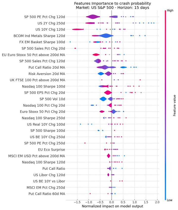
ity. Figure 7 provides the full distribution and is commented
in section 4.3.
Concerning figure 6, we find that the the most significant
feature is the 250 days change in S&P 500 Price Earnings
ratio (the forward 1 Yr Earnings of the index as provided
by Bloomberg). Its correlation with the logit contribution is
negative.
This relationship infers that a positive (resp. negative)
change in P/E over one year lowers (resp. increases) the
Figure 5. Simple strategy probability of crash. It indicates that a positive change in P/E
over a one year horizon translates into a perception of im-
provement in the economic cycle and a positive regime for
value (Shapley, 1953) of a classifier is the average marginal equities. This makes a lot of sense as it is well known that
contribution of the model over the possible different permu- there are cycles of repricing whenever market participants
tations in which the ensemble can be formed (Chalkiadakis anticipate a positive and rising regime in the equity mar-
et al., 2011). It is rigorously defined as follows. kets. In short, when a majority of investors are optimistic, a
Definition 4.1. Shapley value. The Shapley value of binary higher valuation multiple prevail in equities’ market
classifier M in the ensemble M, for the data point level
ensemble game G = (M, v) is defined as By the same token, a positive (resp. negative) change in
X |S|! (|M| − |S| − 1)!
the US 2 Yrs yield over 250 days characterizes a regime
ΦM (v) = (v(S∪{M })−v(S)). of growth (resp. recession) in equities. A positive change
|M|!
S⊆M\{M } in the Bloomberg Base Metals index portrays a positive
regime in equities, thus diminishing the probability of crash.
where S is the subset of features used, v(S) is the predic- The same reasoning applies for Fx Emerging Basket, S&P
tion for features values in set S that are marginalized over Sales evolution, the Euro Stoxx distance to its 200 moving
features that are not included in set S: average. Similarly, the EU Economic Surprise Index is used
to characterize the economic cycle
Z
val(S) = fˆ(x1 , ..., xp )dPx∈X ˆ
/ − E[f (X)]
Interestingly, the Machine Learning approach has identified
the Put/Call ratio as a powerful contrarian indicator, using a
Theoretically, calculating the exact Shapley value for a low level of Put/Call ratio to detect a higher level of crash
model is a hard task and should take O(|M|!) time which in the S&P 500.
is computationally unfeasible in large scale settings. How-
ever, a practical solution is to calculate the approximate Indeed, a persistently low level of Put/Call ratio (as reflected
Shapley values using the conditional expectation instead of by a low 20 days moving average) indicates an excessive
the marginal expectation, which reduces computing time bias of positive investors vs. negative investors and therefore
to O(|M|2 ) and is implemented in most gradient boosting an under-hedged market.
decision trees library such as XGBoost or LightGBM or the The correlation between the Put/Call ratio and the logit
Shap library: https://github.com/slundberg/shap contribution is therefore negative, a low level of the Put/Call
ratio involving an increase in the probability of crash. This
4.2. Shapley interpretation makes a lot of sense. A higher (resp. lower) Risk Aversion
We can rank the Shapley values by order of magnitude accounts for a higher (resp. lower) crash probability and the
importance, defined as the average absolute value of the same relationship is verified with the realized 10 days S&P
Shapley value over the training set of the model. Further- 500 volatility.
more, the Shapley values are correlated with the feature, Last but not least, the Nasdaq 100 is used as a contrarian
therefore enabling to highlight the nature and the strength indicator : the higher the percentage of Nasdaq and the
of the relationship between the logit contribution and the Sharpe Ratio, the higher the crash probability. In general,
feature. As a matter of fact, a positive correlation (resp. neg- the trend of other markets is used in a pro cyclical ways
ative correlation) conveys a positive relationship between
7(Euro Stoxx, BCOM Industrials, FX emerging) whereas the Moving Average of the Put/Call Ratio is used as a contrar-
domestic price indicators are used in a contrarian way (Nas- ian indicator: low values of the indicator reflects an under
daq 100, S&P 500). This is where we can see some strong hedged market and convey an increase in the crash prob-
added value of the machine learning approach that mixes ability whereas elevated values carry a regime of extreme
contrarian and trend following approaches while human stress where hedging strategies prevail thus accounting for a
favor mostly one single approach. decrease in the crash probability. This finding is consistent
with the correlation of -0.88 between the Put/Call ratio and
4.3. Shapley Values’ Distribution the Shapley Values as showed in figure 6. The relationship
between the 20 days moving average of Risk Aversion and
Because some of the features have a strong non linear behav- the logit contribution is also clearly negative: above all,
ior, we also provide in figure 7 the full marginal distribution. lower values of Risk Aversion are related to negative contri-
More precisely, figure 7 displays a more precise relationship bution to crash probability, whereas higher Risk Aversion
between the Shapley values and the whole distribution of accounts for an increase in the crash probability. This rela-
any individual features. tionship is consistent with the correlation of -0.89 displayed
For instance, high 250 days change in P/E ratio represented in figure 6.
in red color has a negative impact on the logit contribution, The use of the change in Nasdaq 100 price over 20 days
everything else being equal. Therefore, an increase in the is confirmed as a contrarian indicator (correlation of -0.89
P/E ratio involves a decrease in the crash probability of S&P in figure 6). As illustrated in Figure 7, negative returns
500 and vice versa. The dependency of the crash probability of the Nasdaq 100 over 20 days are associated with lower
is similar for the change in US 10 Yrs and 2 Yrs yield: the crash probability, everything else being equal. Conversely,
higher (resp. lower) the change in yield, the lower (resp. the most elevated values of Nasdaq 100 20 days returns
higher) the crash probability of S&P 500. produces an increase in the crash probability but in a more
However, the dependency on BCOM Industrial Sharpe ratio muted way. Figure 7 therefore provides an additional infor-
calculated over 120 days is more complex and non linear. mation: negative returns of the Nasdaq 100 are more used
As a matter of fact, low Sharpe ratio of industrial metals than positive returns in the forecast of crash probability.
can have conflicting effects on the crash probability either Conversely, the 20 days Euro Stoxx returns is used in a pro
increasing or decreasing the probability whereas elevated cyclical way as inferred by the correlation -0.85 displayed
Sharpe ratio has always a negative impact on the crash in figure 6. Higher (resp. lower) Euro Stoxx returns are
probability. The same ambiguous dependency is observed associated with a decline (resp. surge) in the crash proba-
against the Sharpe ratio of FX Emerging calculated on a 100 bility. As previously stated, the GBDT model uses non US
days horizon. This behavior confirms the muted correlation markets in a procyclical way but US markets in a contrarian
between the FX EM Sharpe ratio and the Shapley value way and as displayed in figure 7, the type of relationship
although the variable is significant. This complex depen- seems to be univocal.
dency highlights the non linear use of the feature by GBDT
models and the interaction between this feature with other 4.4. Can the machine learning provide an answer to the
features uses by the model. By the same token, the change Covid Equity bubble?
in Sales of S&P 500 over 20 days has not a straightforward
Not only can Shapley values provide a global interpreta-
relationship with the crash probability. First of all, mostly
tion as described in section 4.2 and 7, it can also supply
elevated values of the change in sales are used by the model,
a local interpretation at every single date. Hence we have
shedding light on the conditional use of extreme values of
13 figures ranging from 8 to 20. These figures provide the
the features by the GBDT model. Furthermore, elevated
monthly evolution of the Shapley value over 2020. We can
changes in S&P 500 sales over 20 days are mostly associ-
notice that a lot of features are the same from months to
ated with a diminution of the crash probability but not in
months, indicating a persistence of behavior and importance
every instance.
of features like SP 500 Price Earning percentage over 120
The use of the distance to the Euro Stoxx 50 to its 200 days days, risk aversion, economical cycles variables like indus-
moving average is mostly unambiguous. Most of elevated trial metals and other equity markets as well as central bank
levels in the feature’s distribution involves a decrease in the influenced variables like nominal and real rates and some
crash probability whereas weak levels conveys a bear market technical indicator like put call ratio.
regime and therefore accounts for an increase in the crash
On 1st January 2020, the model was still positive on the
probability. Meanwhile, some rare occurrences of elevated
S&P 500 as the crash probability was fairly low, standing
values of the distance in Euro Stoxx prices’ to their 200 days
at 9.4%. The positive change in P/E at 6% accounted for a
moving average can be associated with higher probability
decrease in the probability, while a risk aversion reflected
of crash highlighting a non linear dependency. The 20 days
8ample liquidity and positive EU Economic Surprise index 15 days.
all reinforced a low probability crash. However, the decline
However, one must be careful and should not be overconfi-
in the US LIBOR is characteristic of a falling economy,
dent about the model forecast. The model presented in the
thus increasing the crash probability. Similarly, the elevated
paper has a short time horizon (15 days), which does not
Put/Call ratio reflected excessive speculative behavior. At
portend any equity evolution on a longer time frame. It may
the beginning of February, the probability, though still mod-
miss certain behavior or new relationships between markets
erate, started to increase slightly. Yet, at the onset of the
as it only monitors 150 variables. More importantly, the
Covid crash, probability increased dramatically on the back
model reasons using only past observations. Should the fu-
of deteriorating dynamics of industrial metals, falling euro
ture be very different from the past, it may wrongly compute
stoxx prices, declining FTSE prices, degradation of EU eco-
crash probabilities influenced by non repeating experience.
nomic surprises and failing S&P 500 P/E. In a nutshell, the
model identified a downturn in the equities’ cycle. This
anticipation eventually proved prescient. Meanwhile, at the 5. Conclusion
start of April 2020, the model eased the crash probability.
In conclusion, in this work, we see that GBDT methods
The Nasdaq Sharpe ratio appeared excessively negative, the
can provide a machine learning answer to the Covid Equity
Put/Call ratio displayed extremely prudent behavior among
Bubble. Using a simple approach of two modes, GBDT is
investors. Contrarian indicators eventually started to bal-
able to learn from past data and classify financial markets
ance pro cyclical indicators, therefore explaining the easing
in normal and crisis regimes. When applied to the S&P
of the crash probability. During several months, the crash
500, the method gives high AUC score providing some
probability stabilized between 20% and 30% until the start
evidence that the machine is able to learn from previous
of July which showed a noticeable decline of probability
crisis. We also report that GBDT report improved accuracy
towards 11.2%. The P/E cycle started to improve and neg-
over other ML methods, as the problem is a higly imbalance
ative signals on base metals and other equities’ dynamics
classification problem with a limited number of observation.
started to improve to the upside. Although the crash proba-
The analysis of Shapley values caters valid and interesting
bility fluctuated, it remained contained though out the rest
explanations of the current Covid equity high valuation. In
of 2020.
particular, the machine is able to find non linear relationships
At the turn of the year 2020, most of signals were positive on between different variables and detects the intervention of
the back on improving Sharpe ratio of Industrial metals, fail- central banks and their accommodative monetary policy that
ing dollar index, easing of Risk Aversion, reflecting ample somehow inflated the current Covid Equity bubble.
liquidity in financial markets, convalescent other equities
markets. For sure, this improving backdrop is moderated References
by lower rates over one year and various small contributors.
Meanwhile, the features’ vote leans towards the bullish side. Aguilar-Rivera, R., Valenzuela-Rendón, M., and Rodrı́guez-
Ortiz, J. Genetic algorithms and darwinian approaches
This rationalization of the post equity bubble does not in financial applications: A survey. Expert Systems with
provide an excuse of the absolute level of equity prices. Applications, 42(21):7684–7697, 2015. ISSN 0957-4174.
Nonetheless, the dynamics of equity prices can clearly be
explained in light of past crises and improving sentiment. Atsalakis, G. S. and Valavanis, K. P. Surveying stock market
For sure, sentiment may have been driven by unprecedented forecasting techniques – part ii: Soft computing methods.
fiscal and monetary interventions but the impact they had Expert Systems with Applications, 36(3, Part 2):5932–
on markets could have been successfully analyzed by a 5941, 2009.
machine learning approach learning only from pretended
episode. Therefore, equity prices may be irrational at the Ballings, M., den Poel, D. V., Hespeels, N., and Gryp, R.
turn of 2020 but dynamics of prices were nonetheless ratio- Evaluating multiple classifiers for stock price direction
nal from a machine learning perspective. prediction. Expert Systems with Applications, 42(20):
7046–7056, 2015. ISSN 0957-4174. doi: https://doi.org/
In summary, machine learning does provide an answer 10.1016/j.eswa.2015.05.013.
thanks to a detailed analysis of the different features. It
does spot that given the level of various indicators and in Benhamou, E., Saltiel, D., Vérel, S., and Teytaud, F.
particular industrial metals, long terms yield, break even BCMA-ES: A bayesian approach to CMA-ES. CoRR,
inflation, that reflect public intervention and accommodative abs/1904.01401, 2019.
monetary policies of central banks that mute and ignore any
offsetting factors like lower rates over one year, the model Benhamou, E., Saltiel, D., Ohana, J.-J., and Atif, J. Detect-
forecast a rather low probability of a large correction over ing and adapting to crisis pattern with context based deep
reinforcement learning, 2020a.
9Benhamou, E., Saltiel, D., Ungari, S., and Mukhopadhyay, Prokhorenkova, L., Gusev, G., Vorobev, A., Dorogush, A. V.,
A. Time your hedge with deep reinforcement learning, and Gulin, A. Catboost: unbiased boosting with categori-
2020b. cal features. In Bengio, S., Wallach, H., Larochelle, H.,
Grauman, K., Cesa-Bianchi, N., and Garnett, R. (eds.),
Benhamou, E., Saltiel, D., Ungari, S., and Mukhopadhyay, Advances in Neural Information Processing Systems, vol-
A. Aamdrl: Augmented asset management with deep ume 31, pp. 6638–6648. Curran Associates, Inc., 2018.
reinforcement learning. arXiv, 2020c.
Rundo, F., Trenta, F., di Stallo, A. L., and Battiato, S. Ma-
Brown, I. and Mues, C. An experimental comparison of chine learning for quantitative finance applications: A
classification algorithms for imbalanced credit scoring survey. Applied Sciences, 9(24):5574, 2019.
data sets. Expert Systems with Applications, 39(3):3446–
3453, 2012. ISSN 0957-4174. Sezer, O. B., Gudelek, M. U., and Ozbayoglu, A. M. Fi-
nancial time series forecasting with deep learning: A
Chalkiadakis, G., Elkind, E., and Wooldridge, M. Computa- systematic literature review: 2005-2019. arXiv preprint
tional Aspects of Cooperative Game Theory. Synthesis arXiv:1911.13288, 2019.
Lectures on Artificial Intelligence and Machine Learning,
5(6):1–168, 2011. Shah, D., Isah, H., and Zulkernine, F. Stock market anal-
ysis: A review and taxonomy of prediction techniques.
Chen, T. and Guestrin, C. Xgboost: A scalable tree boosting International Journal of Financial Studies, 7(2):26, 2019.
system. CoRR, abs/1603.02754, 2016.
Shapley, L. S. A Value for n-Person Games. Contributions
Ke, G., Meng, Q., Finley, T., Wang, T., Chen, W., Ma, to the Theory of Games, 2(28):307–317, 1953.
W., Ye, Q., and Liu, T.-Y. Lightgbm: A highly efficient
Xing, F. Z., Cambria, E., and Welsch, R. E. Natural lan-
gradient boosting decision tree. In Guyon, I., Luxburg,
guage based financial forecasting: a survey. Artificial
U. V., Bengio, S., Wallach, H., Fergus, R., Vishwanathan,
Intelligence Review, 50(1):49–73, 2018.
S., and Garnett, R. (eds.), Advances in Neural Information
Processing Systems, volume 30, pp. 3146–3154. Curran
Associates, Inc., 2017.
Kingma, D. and Ba, J. Adam: A method for stochastic
optimization, 2014.
Krauss, C., Do, X. A., and Huck, N. Deep neural networks,
gradient-boosted trees, random forests: Statistical arbi-
trage on the S&P 500. European Journal of Operational
Research, 259(2):689–702, 2017.
Li, Y. and Ma, W. Applications of artificial neural networks
in financial economics: A survey. In 2010 International
Symposium on Computational Intelligence and Design,
volume 1, pp. 211–214, 2010.
Lundberg, S. and Lee, S.-I. A unified approach to interpret-
ing model predictions, 2017.
Marceau, L., Qiu, L., Vandewiele, N., and Charton, E. A
comparison of deep learning performances with others
machine learning algorithms on credit scoring unbalanced
data. CoRR, abs/1907.12363, 2019.
Mehra, R. and Prescott, E. The equity premium: A puzzle.
Journal of Monetary Economics, 15(2):145–161, 1985.
Nti, I. K., Adekoya, A. F., and Weyori, B. A. A systematic
review of fundamental and technical analysis of stock
market predictions. Artificial Intelligence Review, pp.
1–51, 2019.
10A. Models comparison
Table 1. Model comparison
Model accuracy precision recall f1-score avg precision auc auc-pr
GBDT FS 0.89 0.55 0.55 0.55 0.35 0.83 0.58
Deep LSTM FS 0.87 0.06 0.02 0.05 0.13 0.74 0.56
RBF SVM FS 0.87 0.03 0.07 0.06 0.13 0.50 0.56
Random Forest FS 0.87 0.03 0.07 0.04 0.13 0.54 0.56
Deep FC FS 0.87 0.01 0.02 0.04 0.13 0.50 0.56
Deep LSTM Raw 0.84 0.37 0.33 0.35 0.21 0.63 0.39
RBF SVM Raw 0.87 0.02 0.01 0.05 0.13 0.50 0.36
Random Forest Raw 0.86 0.30 0.09 0.14 0.14 0.53 0.25
GBDT Raw 0.86 0.20 0.03 0.05 0.13 0.51 0.18
Deep FC Raw 0.85 0.07 0.05 0.02 0.13 0.49 0.06
Table 2. Difference between model with features selection and raw model
Model accuracy precision recall f1-score avg precision auc auc-pr
GBDT 0.02 0.35 0.52 0.49 0.23 0.32 0.41
Deep LSTM 0.03 - 0.31 - 0.31 - 0.30 - 0.08 0.11 0.17
RBF SVM - 0.01 0.06 0.01 - - 0.20
Random Forest 0.02 - 0.27 - 0.02 - 0.10 - 0.02 0.01 0.31
Deep FC 0.02 - 0.06 - 0.03 0.02 - 0.01 0.50
11B. Models Understanding with Shapley values
Figure 6. Marginal contribution of features
12Figure 7. Marginal contribution of features with full distribution
13Figure 8. Shapley values for 2020-01-01
14Figure 9. Shapley values for 2020-02-03
15Figure 10. Shapley values for 2020-03-02
16Figure 11. Shapley values for 2020-04-01
17Figure 12. Shapley values for 2020-05-01
18Figure 13. Shapley values for 2020-06-01
19Figure 14. Shapley values for 2020-07-01
20Figure 15. Shapley values for 2020-08-03
21Figure 16. Shapley values for 2020-09-01
22Figure 17. Shapley values for 2020-10-01
23Figure 18. Shapley values for 2020-11-02
24Figure 19. Shapley values for 2020-12-01
25Figure 20. Shapley values for 2020-12-31
26You can also read