Sector models-A toolkit for teaching general relativity: III. Spacetime geodesics
←
→
Page content transcription
If your browser does not render page correctly, please read the page content below

Sector models—A toolkit for teaching general
arXiv:1804.09765v1 [physics.ed-ph] 25 Apr 2018

                                                 relativity: III. Spacetime geodesics
                                                         U Kraus and C Zahn

                                                         Institut für Physik, Universität Hildesheim, Universitätsplatz 1, 31141 Hildesheim,
                                                         Germany
                                                         E-mail: ute.kraus@uni-hildesheim.de, corvin.zahn@uni-hildesheim.de

                                                         Abstract.
                                                         Sector models permit a model-based approach to the general theory of relativity. The
                                                         approach has its focus on the geometric concepts and uses no more than elementary
                                                         mathematics. This contribution shows how to construct the paths of light and free
                                                         particles on a spacetime sector model. Radial paths close to a black hole are used by
                                                         way of example. We outline two workshops on gravitational redshift and on vertical
                                                         free fall, respectively, that we teach for undergraduate students. The workshop on
                                                         redshift does not require knowledge of special relativity; the workshop on particles
                                                         in free fall presumes familiarity with the Lorentz transformation. The contribution
                                                         also describes a simplified calculation of the spacetime sector model that students
                                                         can carry out on their own if they are familiar with the Minkowski metric. The
                                                         teaching materials presented in this paper are available online for teaching purposes
                                                         at www.spacetimetravel.org.

                                                         Keywords: general relativity, geodesics, gravitational redshift, black hole, sector models
Sector models: III. Spacetime geodesics                                                   2

1. Introduction

In view of the goal of teaching introductory general relativity without going beyond
elementary mathematics, we are developing an approach based on a particular class
of physical models, so-called sector models. The approach relies on the fact that
general relativity is a geometric theory and is therefore accessible to intuitive geometric
understanding. In the first part of this series, we have developed sector models as
physical models of curved spaces and spacetimes (Zahn and Kraus 2014, in the following
referred to as paper I). Sector models implement the description of curved spacetimes
used in the Regge calculus (Regge 1961) by way of physical models. Sector models
can be two-dimensional (e.g. a symmetry plane of a spherically symmetric star), three-
dimensional (e.g. the three-dimensional curved space in the exterior region of a black
hole), or 1+1-dimensional (i.e. a spacetime with two spatial dimensions suppressed,
similar to the Minkowski diagrams of special relativity). Figure 1 illustrates the basic
principle using a sphere by way of example: The curved surface is subdivided into
small elements of area, in this case quadrilaterals (figure 1(a)). The edge lengths are
determined for each quadrilateral. Quadrilaterals in the plane are constructed with
the same edge lengths (figure 1(b)). These are the sectors that make up the sector
model. The sector model is an approximation to the curved surface, its accuracy being
determined by the resolution of the subdivision. For pedagogical purposes, a relatively
coarse resolution is useful. Using sector models, the geometry of the respective space
or spacetime can be studied with graphical methods. This includes the construction
of geodesics as described in the second paper of this series (Zahn and Kraus 2018, in
the following referred to as paper II). The construction implements the determination of
geodesics according to the Regge calculus (Williams and Ellis 1981). The basic principle
is illustrated in figure 1(c). Based on the definition of a geodesic as a locally straight
line, the geodesic is drawn using pencil and ruler: Inside a sector, a sector being a
flat element of area, a geodesic is a straight line. When the line reaches the border of
the sector, the neighbouring sector is joined and the line is continued straight across
the border. Sector models are computed true to scale, therefore, the properties read
off from them are quantitatively correct, within the discretization error. The accuracy
achievable for geodesics is studied in paper II.
      General relativity describes the paths of light and free particles as geodesics in
spacetime. This contribution shows how geodesics in spacetime can be constructed using
spacetime sector models as tools. Radial geodesics close to a black hole are used by way
of example. We outline two workshops the way that we teach them for undergraduate
students. In the workshop on gravitational redshift (section 2), null geodesics are
constructed and the phenomenon of gravitational redshift is inferred. The workshop
on radial free fall (section 3) includes the construction of radial timelike geodesics and a
comparison with the Newtonian descriptions of free fall and of tidal forces. Conclusions
and outlook follow in section 4.
Sector models: III. Spacetime geodesics                                                         3

(a)                             (b)                                (c)

              Figure 1. A sector model and the construction of a geodesic using a sphere by way
              of example. The curved surface is subdivided into small elements of area (a). Their
              edge lengths are determined and the sectors are constructed as flat pieces with the
              same edge lengths (b). A geodesic is constructed as a locally straight line using
              pencil and ruler (c).

2. Workshop on gravitational redshift

In this workshop, world lines of light are constructed as geodesics in spacetime. The
construction shows how gravitational redshift arises. A black hole is used by way of
example, because in its vicinity the effects are large and are clearly visible in the
graphical representation. The construction of geodesics is restricted to radial paths;
in the representation of the spacetime the other two spatial directions are suppressed so
that the spacetime sector model is 1+1-dimensional.
     The workshop presumes that the participants are familiar with the concept of a
geodesic as a locally straight line and with sector models as representations of surfaces
with curvature. A knowledge of special relativity is not required for this workshop.
Minkowski diagrams do play a role and if necessary they are explained to the extent
that they are needed in the workshop: Firstly they are introduced as path-time diagrams
that differ from the familiar diagrams used in Newtonian mechanics by the fact that
the vertical axis is the time axis. In order to familiarize the participants with this
representation, we show a diagram with world lines that tell a little story and ask
the participants to recount what happens (an example of such a diagram is available
online, Kraus and Zahn 2018). Secondly, the units of the axes are addressed, being
chosen to make motion at the speed of light run at 45◦ in the diagram. Finally the
terms event, world line and light cone are introduced.

2.1. Redshift close to a black hole
The workshop begins with the explanation that general relativity describes the paths
of light and free particles as geodesics in spacetime. Then a sector model is introduced
that represents the spacetime of a radial ray in the exterior region of a black hole. The
participants can calculate the sector model themselves (section 2.2) or can be provided
with a worksheet (available online, Kraus and Zahn 2018). In a thought experiment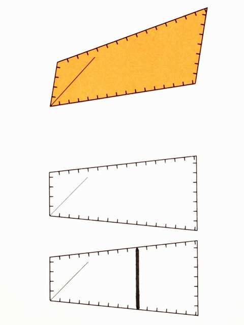
Sector models: III. Spacetime geodesics                                                               4

                                          r                     cT

                     B
             A

                                                                                                     X
(a)                                                             (b)

                 Figure 2. Sector model for the spacetime of a radial ray in the exterior region of
                 a black hole. (a) Radial ray. (b) Spacetime sector model for the segment marked in
                 (a). The edge on the left represents events at point A, the edge on the right events at
                 point B. The diagonal lines mark the light cone. The model can be extended in time
                 by adding identical sectors.

the sector model is created from measurements taken close to a black hole: Astronauts
travel to a black hole and take up positions along a radial ray. They choose a number
of events at these positions and use them as vertices for subdividing the spacetime of
the radial ray into quadrilaterals. In order to define an individual quadrilateral, two
positions are chosen on the radial ray (figure 2(a)). Two events at the inner position and
two at the outer position make up the four vertices. Each quadrilateral is represented
by a sector of a Minkowski space (figure 2(b)); the ensemble of sectors makes up the
sector model.‡ Since the black hole spacetime is static (we consider a non-rotating black
hole), it is possible to choose a subdivision of the spacetime for which the shape of the
sectors is independent of time (see section 2.2). This is here implemented, so that the
sector model can be arbitrarily extended in time by adding identical sectors.
     The first construction on the sector model is the world line of a light signal
propagating radially outwards. Starting from the bottom left corner of the model,
a locally straight line is drawn in the direction of the light cone (figure 3, bottom
line). Within the sector, the line is straight. When the line reaches the border of
the sector, the position of the border point is copied onto the respective border of the
neighbouring sector and the line is continued from there. The borders are provided with
equidistant tick marks to facilitate the transfer of the border points. The direction in
the neighbouring sector is again prescribed by the light cone, since we are concerned
with a world line of light.§
     In the second step the transmission of two consecutive light signals is studied. An
‡ The sector model covers the region from 1.25 to 2.5 Schwarzschild radii in the Schwarzschild radial
coordinate, see section 2.2.
§ Alternatively, one may join the neighbouring sector and then continue the line straight across the
border as described in figure 1. How to join spacetime sectors is described in section 3.1.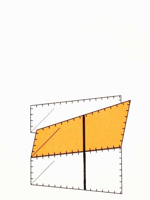
Sector models: III. Spacetime geodesics                                                                5

                    cT
                                                                  ∆t ≈ 3

                            ∆t = 2

                                                                               X

               Figure 3. World lines of two light signals propagating radially outwards. An observer
               at the inner rim of the sectors (left) sends the signals at an interval of two time units.
               An observer at the outer rim (right) receives them about three time units apart.

observer positioned close to the black hole and at a constant distance (point A at the
inner rim of the sectors, see figure 2), sends two light signals outwards, one a short
time after the other. In figure 3 the time interval is two time units. A second observer
positioned farther away from the black hole and also at a constant distance (point B at
the outer rim of the sectors), receives the two signals. In order to find the time interval
of the light signals upon reception, the world line of the other signal is added to the
diagram (figure 3, top line). The interval of the signals can then be read off and amounts
to a little over three time units. If one interprets the two signals as consecutive wave
crests of an electromagnetic wave, one concludes from the diagram that the wave is
received with an increased period by the outer observer. Thus, radiation receding from
a black hole is redshifted. The ratio of the periods Pouter and Pinner at points B and A,
respectively, read off from the construction on p  the sector model, is Pouter /Pinner ≈ 1.5.
The calculated exact value is Pouter /Pinner = (1 − rS /router )/(1 − rS /rinner ) = 1.73,
where rinner = 1.25 rS and router = 2.5 rS are the radial coordinates of points A and B,
respectively. The graphically determined value is too small by 13%; this deviation is
due to the relatively coarse resolution of the sector model.

2.2. Calculation of the spacetime sector model
A simplified calculation of sector models is introduced in paper II (section 2.4) for curved
surfaces and is here extended to the 1+1-dimensional case. This calculation presumes
knowledge of the Minkowski metric. Using the simplified method students can calculate
sector models on their own using elementary mathematics only. This enables them to
use sector models as tools for studying other curved spacetimes when given their metric.
Sector models: III. Spacetime geodesics                                                           6

        ct
    2.5 rS
                                                  cT
                                                                                       C
                                                            D
  1.25 rS                                                                 h
                       D     C                              b1                         b2
                                                             A
                                                                                       B
                       A     B
        0
             0     1.25 rS 2.5 rS 3.75 rS r                                                   X
  (a)                                             (b)

                 Figure 4. Calculation of the spacetime sector model of a radial ray. (a) The
                 subdivision of the spacetime in coordinate space. (b) Each sector is constructed in
                 the shape of a symmetric trapezium.

The approximations of the simplified method are discussed in paper II.
      The starting point of the construction is the metric
                               rS  2 2         1
               ds2 = − 1 −           c dt +             dr 2                             (1)
                                r             1 − rS /r
with the usual Schwarzschild coordinates t and r and the Schwarzschild radius rS =
2GM/c2 of the central mass M, where G is the gravitational constant and c the speed
of light.
      In space the sector model represents a segment of a radial ray from r = 1.25 rS to
r = 2.5 rS with coordinate length ∆r = 1.25 rS. The time coordinate t is subdivided into
segments of length ∆t with c∆t = 1.25 rS (figure 4(a)). Since the metric is independent
of the time coordinate, only a single segment in time needs to be calculated.
      The calculation of the edge intervals yields
                                   rS  2 2
               ∆s2t (r) = − 1 −         c ∆t          (∆r = 0)                           (2)
                                    r
for the timelike edges and
                             1
               ∆s2r =                 ∆r 2      (∆t = 0)                                 (3)
                        (1 − rS /rm )
for the spacelike edges, where the metric coefficient is evaluated at the mean coordinate
rm = (r1 +r2 )/2 with the coordinates r1 and r2 of the associated vertices. Since the sector
model is a column of identical sectors, each sector is constructed with the corresponding
time symmetry: As shown in figure 4(b),  p the bases of a trapezium arepdrawn in direction
of the time axis with the lengths b1 = −∆st (r = 1.25 rS ) and b2 = −∆s2t (r = 2.5 rS).
                                                 2

The height h of the trapezium is determined from the condition that the lateral sides
have the interval ∆s2r (figure 4(b)):
                                   2
                  2         b2 − b1
               ∆sr = −                  + h2 .                                           (4)
                               2
The result is the sector shown in figure 2.
Sector models: III. Spacetime geodesics 7
ct ct (x′ = 0) (x′ = l0 )
(t′ = t0 )
ct0 γ −1 ct0
θ (t′ = 0)
v
tan θ = c
0 0 θ
0 x 0 x
l0 γ −1 l0
(a) (b)
Figure 5. Graphic representation of a spacetime sector in two different reference
frames. The events are located inside a spaceship of length l0 at spaceship proper
times between zero and t0 . (a) Representation in the rest frame of the spaceship. (b)
Representation in the restp frame of a space station that the spaceship passes with
velocity v = 0.3 c (γ = 1/ 1 − v 2 /c2 ).
3. Workshop on particle paths
In this workshop world lines are constructed for freely falling particles close to a black
hole. As in the previous section the study is restricted to radial paths, so that it is
possible to use a 1+1-dimensional spacetime sector model. By means of the particle
paths, the connection between the relativistic and the classical descriptions of motion
in a gravitational field is pointed out. The workshop presumes that the participants are
familiar with the Lorentz transformation.
3.1. The construction of timelike geodesics
To study the paths of freely falling particles in the vicinity of a black hole, their world
lines are constructed on a sector model. As in the previous examples, the geodesics are
drawn as straight lines within each sector and after reaching the boundary are continued
in the neighbouring sector. Other than for the null geodesics discussed in section 2, the
direction in the neighbouring sector is not predetermined by the light cone. Therefore,
it is necessary to join the neighbouring sector and to continue the line straight across
the boundary. The joining of two sectors is more complex in spacetime than in the
purely spatial case. Clearly, rotating the neighbouring sector into a suitable position is
not an option: Since the speed of light has the same value in both sectors, their light
cones must coincide. This fixes the orientation of the neighbouring sector.
In the workshop we use a specific example for a spacetime sector in order to
introduce the way that neighbouring sectors can be joined. We consider a long and
very thin spaceship of rest length l0 . We define a spacetime sector that is made up ofSector models: III. Spacetime geodesics 8
Figure 6. Joining two spacetime sectors of the sector model shown in figure 2. The
upper sector has been Lorentz-transformed in such a way that it can be joined to the
lower sector (v/c = 0.21).
(a) (b) (c)
Figure 7. Construction of a geodesic on the spacetime sector model. (a) A sector
that has undergone Lorentz transformation serves as transfer sector (in colour). (b)
The geodesic is continued straight onto the transfer sector. (c) The line is copied from
the transfer sector onto the neighbouring sector in the original symmetric shape.
all events that are inside the spaceship and at spaceship proper times between zero and
t0 . The participants draw this spacetime sector in a Minkowski diagram, first in the
rest frame of the spaceship (figure 5(a)), then in the rest frame of a space station that
the spaceship passes at constant relative velocity (figure 5(b)). The geometric shape of
the sector, i.e., the geometric shape drawn on paper and understood in the euclidean
sense, clearly depends on the frame of reference. Figures 5(a) and (b) are two different
representations of one and the same spacetime sector. One turns into the other under
a Lorentz transformation.
This permits the joining of sectors: The neighbouring sector is brought into the
appropriate form by Lorentz transformation (figure 6). Thus, the transformation that
permits the joining of the neighbouring sector is a rotation in the spatial case and a
Lorentz transformation in the spacetime case.
When drawing geodesics, it is convenient to use a transformed sector in the role ofSector models: III. Spacetime geodesics 9
(a) (b)
Figure 8. Vertical free fall. (a) A geodesic constructed on the sector model. (b)
When all sectors are joined, the world line can clearly be seen to be straight.
transfer sector (paper II, section 2.3): When a geodesic reaches the border of a sector
(figure 7(a)), it is continued as a straight line across the border onto the transfer sector
joined to the respective edge (figure 7(b)) and is then transferred onto the neighbouring
sector in its original shape (figure 7(c)). This transfer amounts to reversing the Lorentz
transformation. In doing so, straight lines are mapped onto straight lines. Therefore,
using the tick marks at the borders, the end points of the line are transferred onto the
target sector and are then connected by a straight line (figure 7(c)).
3.2. Vertical free fall
Close to a black hole, a particle is thrown upwards. Its path is to be determined.
Intuitively, it is clear that the particle reaches a maximum height and then falls back
down (provided its initial velocity is less than the escape velocity).
In the relativistic description, the particle, being in free fall, follows a geodesic, i.e.,
its world line is locally straight. How can these two statements—straight world line on
the one hand and up-and-down motion on the other hand—be compatible?
For the construction of the world line, the sector model shown in figure 2 is used
with six rows plus an appropriately transformed transfer sector (figure 6). After choosing
an initial position and a timelike outward direction, the world line is constructed as a
geodesic on the sector model (figure 8(a)): The locally straight line at first leads away
from the black hole and then comes closer again. The spacetime geodesic thus provides
the expected up-and-down motion in space. In addition, figure 8(b) shows the sector
model with all the sectors joined, so that the straightness of the line is obvious. In orderSector models: III. Spacetime geodesics 10
ct
2.5 rS
1.25 rS
0
0 1.25 rS 2.5 rS 3.75 rS r
(a) (b)
Figure 9. Spacetime sector model for a radial ray in the exterior region of a black hole.
(a) Subdivision of the spacetime in coordinate space. (b) Sectors in symmetric form
(bottom) and suitably Lorentz-transformed transfer sectors (top). This is an extension
of the model shown in figure 2 by a second column with the associated transfer sector
(right hand side, v/c = 0.067). The model can be extended in time by adding identical
rows.
to draw the geodesic at a stretch as in this figure, one needs several representations of
the sector that are obtained by Lorentz transformations with different velocities. The
construction on the sector model displays both the straight line in spacetime and the
up-and-down motion in space, and so makes the connection between them quite clear.
3.3. Tidal forces and the curvature of spacetime
When the present workshop on particle paths is combined with the workshop on
curvature described in paper I, it is possible to illustrate the physical significance of
spacetime curvature with the help of geodesics. For this purpose a second column is
added to the sector model shown in figure 2, so that the model now covers the radial
ray between 1.25 rS and 3.75 rS in two columns (figure 9). The model is used with eight
rows plus a transfer sector for each column.
In a local inertial frame momentarily at rest with respect to the black hole, we
consider two particles that are slightly displaced in the radial direction. They are
released from rest simultaneously, so that they fall one after another radially into
the black hole. In the classical description the gravitational force decreases outwards.
Therefore, at each instant the outer particle experiences a smaller acceleration than the
inner one, so that the two freely falling particles are accelerated relative to each other:
As a result of tidal forces, the relative velocity of the particles increases.
In the general relativistic description, the world lines of the two particles are
geodesics that are initially parallel. These geodesics are constructed on the sector model
(figure 10). Both world lines start in the direction of the local time axis (figure 10,
bottom row). The two initially parallel world lines diverge more and more indicating a
relative velocity that increases.Sector models: III. Spacetime geodesics 11
Figure 10. The world lines of two particles that are simultaneously released from rest
and fall one after another towards a black hole.
The construction elucidates the origin of the divergence: The world lines are parallel
up to the point where they pass a vertex on different sides (figure 10, row 4 to row 5 from
the bottom). Each additional vertex between the world lines increases the difference in
direction, i.e., increases the relative velocity.
Figure 11 shows the run of a pair of geodesics close to a single vertex in more detail.
For clarity, sectors with double coordinate length in time are used (c∆t = 2.5 rS ). In
figures 11(a) and (b) the sectors are joined along the geodesic on the left and on the
right, respectively (the upper row being suitably Lorentz-transformed as a whole in each
case); in figure 11(c) the sectors are arranged symmetrically.
As described in paper I, in a sector model the so-called deficit angles of the vertices
represent curvature. The deficit angle of the vertex considered here is apparent in
figures 11(a) and (b) as the gap that remains when the four adjacent sectors are joined
around the vertex. This deficit angle is in a spacelike direction and is positivek; with the
metric signature used here, by convention, this means positive spacetime curvature. By
construction, the angle between the two lines behind the vertex depends on the deficit
angle. Thus, figures 10 and 11 show that positive spacetime curvature is linked with
the divergence of initially parallel world lines; the opposite holds in the case of negative
curvature. Spacetime curvature is less intuitive than spatial curvature. However, the
k The deficit angle is positive if a wedge-shaped gap remains after joining all adjacent sectors. It is
negative if, after joining all the sectors except one, the remaining space is too small to accommodate
the last sector.Sector models: III. Spacetime geodesics 12
(a) (b) (c) (d)
Figure 11. Initially parallel geodesics that pass a vertex on opposite sides
subsequently are no longer parallel. In (a) the sectors are joined along the geodesic
on the left and in (b) along the geodesic on the right; in (c) they are arranged
symmetrically. (d) Spacelike geodesics show the opposite behaviour. (Sector model as
in figure 9, but with double coordinate length in time, c∆t = 2.5 rS .)
run of neighbouring geodesics provides a criterion that can be understood geometrically.
Thus the construction shows how the relative acceleration of the two particles comes
about in the relativistic description. It can be traced back to the deficit angles at the
vertices, i.e. to curvature. This elucidates the physical meaning of spacetime curvature:
It corresponds to the Newtonian tidal force.
In addition, figure 11(d) shows the behaviour of initially parallel spacelike geodesics
near the same vertex: After the vertex they converge. The opposing behaviour of
timelike and spacelike geodesics reflects the corresponding properties of the deficit angles
in timelike and spacelike directions, respectively (paper I, section 4).
3.4. The construction of geodesics using transfer double sectors
When geodesics are constructed as described above, in some cases the line segment
within a sector is very short because it passes close to a vertex (e.g., in figure 10,
4th row from the bottom, left line). In this case the further construction is quite
imprecise because the subsequent direction is determined from this short segment. The
problem can be solved by using not a single transfer sector but a double one (figure 12).
This is built by joining a sector of the neighbouring column, after appropriate Lorentz
transformation, to a transfer sector. The line on the double sector is then longer and
the construction is more precise. In the workshops we first introduce the single transfer
sectors of figure 9. When the procedure is clear, we switch to the double sectors of
figure 12.Sector models: III. Spacetime geodesics 13
(a) (b)
Figure 12. Transfer double sectors. (a) For the left column of the sector model of
figure 9, (b) for the right column.
4. Conclusions and outlook
4.1. Summary and pedagogical comments
In this contribution we have shown how paths of light and free particles can be
constructed on spacetime sector models. The construction of null geodesics directly
leads to the phenomenon of gravitational redshift (section 2.1). The construction of
timelike geodesics shows that describing the motion of a particle in free fall as a geodesic
in spacetime, provides the expected up-and-down motion in space (section 3.2). By
studying timelike geodesics of neighbouring particles, the connection between spacetime
curvature and Newtonian tidal forces is revealed (section 3.3).
In connection with the use of spacetime sector models one can discuss the
equivalence principle that is expressed here in a clear way. It states that in sufficiently
small regions of a curved spacetime Minkowski geometry applies and that locally all
physical phenomena are described by the special theory of relativity. In a sector model
each sector constitutes such a small region. The curved spacetime is explicitly made up
of local regions with Minkowski geometry. In the sector model one can advance through
curved spacetime by passing from one Minkowski sector to the next. The local validity
of special relativity is directly implemented on sector models, when the world lines of
light and free particles are drawn as straight line segments within a sector.
The sector model used here represents a 1+1-dimensional subspace of the
Schwarzschild spacetime. It allows the construction of radial world lines. Non-radial
world lines can in principle be determined in a 2+1-dimensional sector model, but an
implementation with models made from paper or cardboard does not appear practicable.
An implementation using three-dimensional interactive computer visualization is being
studied.
The workshops on redshift and particle paths presented here were developed
and tested at Hildesheim University in the context of an introduction to general
relativity for pre-service physics teachers (Zahn and Kraus 2013, Kraus et al 2018).
This introductory course uses the model-based approach described here including the
calculation of the relevant sector models from their metrics. The calculation of sector
models is introduced step by step starting with the sphere via the equatorial planeSector models: III. Spacetime geodesics 14
of a black hole (paper II, section 2.4) to the spacetime of a radial ray (section 2.2).
The course uses the material described in papers I to III plus material from part four
currently in preparation. In the homework problems and the tutorials, the students
calculate sector models for other metrics on their own and use them to study curvature
and geodesics. Thus, in the model-based course students are taught the necessary skills
for studying (to a certain extent) the physical phenomena associated with a given metric.
Answers are here obtained graphically that in a standard university course would be
found by calculations. An example of a problem that can be solved with the methods
of the model-based course is the following: ‘The metric of a radial ray in an expanding
spacetime is given as ds2 = −c2 dt2 + (t/T0 )2 dx2 , where T0 is a constant. Two observers,
each at a constant coordinate x, exchange light signals. Will they observe a redshift?’
Details on the pre-service teacher course and its evaluation are presented by Kraus et al
(2018).
Other possible uses, e.g. in an astronomy club at school, exist, in particular, for
the workshop on redshift because it does not require the participants to have knowledge
of special relativity. Also, all of the material can be used as a supplement to a
mathematically oriented university course and help to strengthen geometric insight.
4.2. Comparison with other graphic approaches
Sector models provide a graphic representation of spacetime geodesics. Other graphic
representations of geodesics in spacetime have been described using embedding surfaces
(Marolf 1999, Jonsson 2001, 2005). Just as the sector models presented here, these
representations are limited to 1+1-dimensional spacetimes. A related representation
of geodesics is the construction on so-called wedge maps developed by diSessa (1981).
This construction is derived from the Regge calculus and is carried out numerically.
The calculation is also described for 2+1-dimensional spacetimes; light deflection and
redshift are discussed.
In comparison to embedding surfaces and also to wedge maps, the calculation and
use of sector models is more elementary. For a spacetime model, only a basic knowledge
of special relativity is necessary; the determination of geodesics is carried out graphically
and the only mathematical concept that goes beyond elementary mathematics as taught
at school is the concept of the metric. Sector models can easily be constructed and since
they are readily duplicated, all participants of a course can carry out the construction
of geodesics themselves on their own models.
4.3. Outlook
In the model-based approach described here, sector models are the basis for answers
to the three fundamental questions raised in paper I concerning the nature of a curved
spacetime, the laws of motion, and the relation between the distribution of matter and
the curvature of spacetime. In paper I curved spaces and spacetimes are represented as
sector models. In paper II and the present contribution geodesics are studied as paths ofREFERENCES 15 light and free particles. Part four of this series will be on the relation between curvature and the distribution of matter. References diSessa A 1981 An elementary formalism for general relativity Am. J. Phys. 49 (5) 401–11 Jonsson R M 2001 Embedding spacetime via a geodesically equivalent metric of euclidean signature Gen. Rel. Grav. 33 (7) 1207–35 Jonsson R M 2005 Visualizing curved spacetime Am. J. Phys. 73 (3) 248–60 Kraus U, Zahn C, Reiber T and Preiß S 2018 A model-based general relativity course for physics teachers, submitted Kraus U and Zahn C 2018 Online resources for this contribution www.spacetimetravel.org/sectormodels3 Marolf D 1999 Spacetime embedding diagrams for black holes Gen. Rel. Grav. 31 (6) 919–44 Regge T 1961 General relativity without coordinates Il Nuovo Cimento 19 558–71 Williams R M and Ellis G F R 1981 Regge Calculus and Observations. I. Formalism and Applications to Radial Motion and Circular Orbits Gen. Rel. Grav. 13 (4) 361–95 Zahn C and Kraus U 2013 Bewegung im Gravitationsfeld in der Allgemeinen Relativitätstheorie – ein neuer Zugang auf Schulniveau PhyDid B DD 17.13 Zahn C and Kraus U 2014 Sector models—A toolkit for teaching general relativity: I. Curved spaces and spacetimes Eur. J. Phys. 35 (5) 055020 Online version with supplementary material: www.spacetimetravel.org/sectormodels1 (paper I) Zahn C and Kraus U 2018 Sector models—A toolkit for teaching general relativity: II. Geodesics, submitted Online version with supplementary material: www.spacetimetravel.org/sectormodels2 (paper II)
Sektormodelle – Ein Werkzeugkasten zur
arXiv:1804.09765v1 [physics.ed-ph] 25 Apr 2018

                                                 Vermittlung der Allgemeinen Relativitätstheorie:
                                                 III. Geodäten in der Raumzeit
                                                         U Kraus und C Zahn

                                                         Institut für Physik, Universität Hildesheim, Universitätsplatz 1, 31141 Hildesheim
                                                         E-mail: ute.kraus@uni-hildesheim.de, corvin.zahn@uni-hildesheim.de

                                                         Zusammenfassung.
                                                         Sektormodelle ermöglichen einen modellbasierten Zugang zur Allgemeinen Relati-
                                                         vitätstheorie, der auf das Verständnis der geometrischen Konzepte abzielt und in seinen
                                                         mathematischen Anforderungen nicht über Schulmathematik hinausgeht. Dieser Bei-
                                                         trag zeigt, wie die Bahnen von Licht und freien Teilchen auf einem raumzeitlichen
                                                         Sektormodell konstruiert werden können. Als Beispiel dienen radiale Bahnen in der
                                                         Nähe eines Schwarzen Lochs. Wir beschreiben zwei Workshops zu den Themen gravi-
                                                         tative Rotverschiebung sowie radialer freier Fall, die wir in dieser Form mit Bachelor-
                                                         studierenden durchführen. Der Workshop zur Rotverschiebung setzt keine Kenntnisse
                                                         der Speziellen Relativitätstheorie voraus; in dem Workshop zum freien Fall wird die
                                                         Lorentztransformation als bekannt vorausgesetzt. Der Beitrag beschreibt auch eine ver-
                                                         einfachte Berechnung des verwendeten raumzeitlichen Sektormodells, die von Teilneh-
                                                         mer/innen selbstständig durchgeführt werden kann, falls sie mit der Minkowskimetrik
                                                         vertraut sind. Die vorgestellten Materialien stehen online unter
                                                         www.tempolimit-lichtgeschwindigkeit.de für den Unterricht zur Verfügung.
Sektormodelle: III. Geodäten in der Raumzeit 2
1. Einleitung
Im Hinblick auf das Ziel, die Grundlagen der Allgemeinen Relativitätstheorie
zu vermitteln und dabei in den mathematischen Anforderungen nicht über
Schulmathematik hinauszugehen, entwickeln wir einen Zugang, der auf speziellen
Anschauungsmodellen, sogenannten Sektormodellen, basiert. Dahinter steht der
Grundgedanke, dass die Allgemeine Relativitätstheorie eine geometrische Theorie ist,
die deshalb der geometrischen Anschauung zugänglich ist. Im ersten Teil dieser Folge
von Beiträgen haben wir Sektormodelle als Anschauungsmodelle von gekrümmten
Räumen und Raumzeiten entwickelt (Zahn und Kraus 2014, im Folgenden als Teil I
bezeichnet). Sektormodelle setzen die Darstellung gekrümmter Raumzeiten im Regge-
Kalkül (Regge 1961) in Form von gegenständlichen Modellen um. Sektormodelle
können zweidimensional sein (z. B. eine Symmetrieebene eines kugelsymmetrischen
Sterns), dreidimensional (z. B. der gekrümmte dreidimensionale Raum um ein
Schwarzes Loch) oder 1+1-dimensional (d. h. eine Raumzeit, in der zwei räumliche
Dimensionen unterdrückt werden, ähnlich den Minkowskidiagrammen der Speziellen
Relativitätstheorie). Das Prinzip zeigt Abb. 1 am Beispiel der Kugeloberfläche: Die
gekrümmte Fläche wird in kleine Bereiche zerlegt, in diesem Beispiel in Vierecke
(Abb. 1(a)). Für alle Vierecke werden die Kantenlängen bestimmt. In der Ebene
werden Vierecke mit denselben Kantenlängen konstruiert (Abb. 1(b)). Dies sind die
Sektoren, die das Sektormodell bilden. Das Sektormodell stellt die gekrümmte Fläche
näherungsweise dar. Die Güte der Annäherung ist durch die Feinheit der Unterteilung
bestimmt. Für didaktische Zwecke ist eine relativ grobe Unterteilung sinnvoll. An
Sektormodellen kann man die Geometrie der dargestellten Räume und Raumzeiten mit
grafischen Methoden untersuchen. Dazu gehört die Konstruktion von Geodäten, die im
zweiten Teil dieser Folge (Zahn und Kraus 2018, im Folgenden als Teil II bezeichnet)
beschrieben wird. Die Konstruktion ist eine zeichnerische Umsetzung der Bestimmung
von Geodäten im Regge-Kalkül (Williams und Ellis 1981). Das prinzipielle Vorgehen
zeigt Abb. 1(c). Ausgehend von der Definition einer Geodäte als einer lokal geraden
Linie wird die Geodäte mit dem Lineal konstruiert: Innerhalb eines Sektors, der ja ein
ebenes Flächenstück ist, ist eine Geodäte eine gerade Linie. Wenn die Geodäte den
Rand des Sektors erreicht, wird der Nachbarsektor angelegt und die Linie wird über die
Kante hinweg geradlinig fortgesetzt. Sektormodelle werden maßstabsgetreu berechnet,
so dass die geometrischen Eigenschaften, die man an ihnen abliest, im Rahmen
des Diskretisierungsfehlers auch quantitativ korrekt sind. Für Geodäten erzielbare
Genauigkeiten werden in Teil II untersucht.
Die Bahnen von Licht und freien Teilchen werden in der Allgemeinen
Relativitätstheorie als Geodäten in der Raumzeit beschrieben. Dieser Beitrag zeigt, wie
man mithilfe von Sektormodellen Geodäten in der Raumzeit zeichnerisch bestimmen
kann. Als Beispiel dienen radiale Geodäten in der Nähe eines Schwarzen Lochs.
Wir stellen zwei Workshops vor, die wir in dieser Form mit Bachelorstudierenden
durchführen. Im Workshop zur gravitativen Rotverschiebung (Abschnitt 2) werdenSektormodelle: III. Geodäten in der Raumzeit 3
(a) (b) (c)
Abbildung 1. Sektormodell und Konstruktion von Geodäten am Beispiel der
Kugeloberfläche. Die gekrümmte Fläche wird in kleine Bereiche zerlegt (a), deren
Kantenlängen bestimmt werden. Die Sektoren werden als ebene Flächenstücke mit
denselben Kantenlängen konstruiert (b). Eine Geodäte wird als lokal gerade Linie mit
dem Lineal gezeichnet (c).
Nullgeodäten konstruiert, an denen die Rotverschiebung verdeutlicht wird. Der
Workshop zum radialen freien Fall (Abschnitt 3) beinhaltet die Konstruktion von
radialen zeitartigen Geodäten und den Vergleich mit der Newtonschen Beschreibung
des freien Falls sowie der Gezeitenkräfte. Fazit und Ausblick folgen in Abschnitt 4.
2. Workshop Rotverschiebung
In diesem Workshop werden Weltlinien von Licht als Geodäten in der Raumzeit
konstruiert. Daran wird das Zustandekommen der gravitativen Rotverschiebung
verdeutlicht. Als Beispiel dient die Raumzeit eines Schwarzen Lochs, weil die Effekte
dort groß und grafisch gut darstellbar sind. Es werden nur radiale Bahnen betrachtet;
bei der Darstellung der Raumzeit werden die anderen Raumrichtungen unterdrückt, so
dass das raumzeitliche Sektormodell 1+1-dimensional ist.
Der Workshop setzt voraus, dass den Teilnehmer/innen der Begriff der Geodäte
als einer lokal geraden Linie sowie Sektormodelle zur Darstellung von Flächen mit
Krümmung bekannt sind. Vorkenntnisse in Spezieller Relativitätstheorie sind für diesen
Workshop nicht erforderlich. Minkowskidiagramme spielen eine Rolle und bei Bedarf
werden sie zu Beginn des Workshops im benötigten Umfang erläutert: Es wird erstens
erklärt, dass es sich um Raum-Zeit-Diagramme handelt, die sich von den aus der
Mechanik bekannten Diagrammen dadurch unterscheiden, dass die senkrechte Achse
die Zeitachse ist. Um die Teilnehmer/innen mit dieser Darstellung vertraut zu machen,
zeigen wir ein Diagramm mit Weltlinien und lassen die darin dargestellte Geschichte
erzählen (ein Beispiel steht online zur Verfügung, Kraus und Zahn 2018). Zweitens wird
auf die Skalierung der Achsen eingegangen, die so gewählt wird, dass Bewegungen mit
Lichtgeschwindigkeit im Diagramm unter 45◦ verlaufen. Schließlich werden die Begriffe
Ereignis, Weltlinie und Lichtkegel eingeführt.Sektormodelle: III. Geodäten in der Raumzeit 4
r cT
B
A
X
(a) (b)
Abbildung 2. Sektormodell für die Raumzeit eines radialen Strahls im Außenraum
eines Schwarzen Lochs. (a) Radialer Strahl. (b) Raumzeitliches Sektormodell für den
in (a) kenntlich gemachten Abschnitt. Die linke Kante stellt Ereignisse an Punkt A
dar, die rechte Kante an Punkt B. Die diagonalen Linien markieren die Lichtkegel. Das
Modell kann in Zeitrichtung durch identische Sektoren beliebig erweitert werden.
2.1. Rotverschiebung in der Nähe eines Schwarzen Lochs
Der Workshop beginnt mit der Erläuterung, dass die Allgemeine Relativitätstheorie
die Bahnen von Licht und freien Teilchen als Geodäten in der Raumzeit beschreibt.
Es wird dann ein Sektormodell vorgestellt, das die Raumzeit eines radialen Strahls
im Außenraum eines Schwarzen Lochs darstellt. Die Teilnehmer/innen können das
Sektormodell selbst berechnen (Abschnitt 2.2) oder eine Vorlage verwenden (online
verfügbar, Kraus und Zahn 2018). Im Gedankenexperiment entsteht das Sektormodell
aus Messungen in der Nähe eines Schwarzen Lochs: Astronauten reisen zu dem
Schwarzen Loch und positionieren sich dort längs eines radialen Strahls. Sie wählen
eine Reihe von Ereignissen aus und nutzen sie als Eckpunkte um die Raumzeit des
radialen Strahls in Vierecke einzuteilen. Zur Definition eines einzelnen Vierecks werden
zwei Positionen auf dem radialen Strahl ausgewählt (Abb. 2(a)). Zwei Ereignisse an der
inneren sowie zwei an der äußeren Position bilden die vier Eckpunkte. Der viereckige
Ausschnitt der gekrümmten Raumzeit wird durch einen Sektor eines Minkowskiraums
dargestellt (Abb. 2(b)); die Gesamtheit der Sektoren bildet das Sektormodell.‡ Da
die Raumzeit des Schwarzen Lochs statisch ist (wir betrachten ein nichtrotierendes
Schwarzes Loch), kann man eine Darstellung wählen, in der die Form der Sektoren
von der Zeit unabhängig ist (s. Abschnitt 2.2). Dies wurde hier umgesetzt, so dass das
Sektormodell in Zeitrichtung durch weitere identische Sektoren beliebig erweitert werden
kann.
Auf dem Sektormodell wird als erstes die Weltlinie eines Lichtsignals konstruiert,
das radial nach außen läuft. Ausgehend von dem Startpunkt in der linken unteren Ecke
‡ Das Sektormodell überdeckt den Bereich von 1,25 bis 2,5 Schwarzschildradien in der
Schwarzschildschen Radialkoordinate, s. Abschnitt 2.2.Sektormodelle: III. Geodäten in der Raumzeit 5
cT
∆t ≈ 3
∆t = 2
X
Abbildung 3. Weltlinien zweier Lichtsignale, die radial nach außen laufen. Ein
Beobachter am Innenrand der Sektorspalte (links) sendet die Signale im Abstand
von zwei Zeiteinheiten aus. Ein Beobachter am Außenrand (rechts) empfängt sie im
Abstand von ca. drei Zeiteinheiten.
des Modells wird eine lokal gerade Linie gezeichnet, die in Richtung des Lichtkegels
verläuft (Abb. 3, untere Linie). Innerhalb eines Sektors ist die Linie gerade. Erreicht
man beim Zeichnen den Rand, so wird die Linie im Nachbarsektor fortgesetzt: Die
Position am Rand wird auf den entsprechenden Rand des Nachbarsektors übertragen;
zur Unterstützung tragen die Kanten äquidistante Markierungen. Die Richtung im
Nachbarsektor ist, da es sich um eine Weltlinie von Licht handelt, durch den Lichtkegel
vorgegeben.§
Im zweiten Schritt wird die Übermittlung von zwei aufeinanderfolgenden
Lichtsignalen untersucht. Ein Beobachter, der sich nahe am Schwarzen Loch in einer
festen Entfernung (Punkt A am Innenrand der Sektorspalte) befindet, sendet zwei
Lichtsignale in kurzem zeitlichem Abstand nach außen. In Abb. 3 beträgt dieser Abstand
zwei Zeiteinheiten. Ein zweiter Beobachter, der sich weiter außen ebenfalls in fester
Entfernung zum Schwarzen Loch befindet (Punkt B am Außenrand der Sektorspalte),
empfängt die beiden Signale. Um festzustellen, in welchem zeitlichen Abstand der
äußere Beobachter die Signale erhält, wird die Weltlinie des zweiten Signals hinzugefügt
(Abb. 3, obere Linie). Man erkennt, dass der zeitliche Abstand am Außenrand der Spalte
rund drei Zeiteinheiten beträgt. Wenn man die beiden Signale als aufeinanderfolgende
Wellenberge einer elektromagnetischen Welle deutet, dann folgt aus der Konstruktion,
dass die Welle außen mit einer vergrößerten Periode empfangen wird. Strahlung, die
sich vom Schwarzen Loch entfernt, wird also rotverschoben. Das Verhältnis der Perioden
Paußen und Pinnen am äußeren Punkt B bzw. am inneren Punkt A ergibt sich aus der
§ Alternativ kann man den Nachbarsektor anlegen und die Geodäte geradlinig fortsetzen, wie in Abb. 1
beschrieben. Das Vorgehen beim Anlegen von raumzeitlichen Sektoren wird in Abschnitt 3.1 erläutert.Sektormodelle: III. Geodäten in der Raumzeit 6
ct
2.5 rS
cT
C
D
1.25 rS h
D C b1 b2
A
B
A B
0
0 1.25 rS 2.5 rS 3.75 rS r X
(a) (b)
Abbildung 4. Zur Berechnung des raumzeitlichen Sektormodells eines radialen
Strahls. (a) Die Aufteilung der Raumzeit im Koordinatenraum. (b) Jeder Sektor wird
als symmetrisches Trapez konstruiert.
Konstruktion zu Paußen /Pinnen ≈ 1,5. Der berechnete exakte Wert ist Paußen /Pinnen =
p
(1 − rS /raußen )/(1 − rS /rinnen ) = 1,73 wobei rinnen = 1,25 rS und raußen = 2,5 rS die
Radialkoordinaten der Punkte A und B sind. Der grafisch bestimmte Wert ist 13% zu
klein; diese Abweichung ist der relativ groben Auflösung des Sektormodells geschuldet.
2.2. Berechnung des raumzeitlichen Sektormodells
Eine vereinfachte Berechnung von Sektormodellen wird in Teil II (Abschnitt 2.4)
eingeführt und hier auf eine 1+1-dimensionale gekrümmte Raumzeit übertragen. Diese
Berechnung setzt die Kenntnis der Minkowskimetrik voraus. Mit dem vereinfachten
Verfahren kann das Sektormodell von den Teilnehmer/innen des Workshops mit Mitteln
der Schulmathematik selbst berechnet werden. Dies versetzt sie in die Lage, auch andere
gekrümmte Raumzeiten ausgehend von deren Metrik mit Hilfe von Sektormodellen zu
untersuchen. Die mit dem vereinfachten Verfahren verbundenen Näherungen werden in
Teil II diskutiert.
Die Konstruktion geht von der Metrik
2
rS 2 2 1
ds = − 1 − c dt + dr 2 (1)
r 1 − rS /r
aus, wobei t und r die üblichen Schwarzschildkoordinaten sind und rS = 2GM/c2 der
Schwarzschildradius der Zentralmasse M mit der Newtonschen Gravitationskonstanten
G und der Lichtgeschwindigkeit c.
Das Sektormodell stellt räumlich einen Abschnitt eines radialen Strahls zwischen
r = 1,25 rS und r = 2,5 rS dar, der die Koordinatenlänge ∆r = 1,25 rS hat. Die
Zeitkoordinate t wird in Abschnitte der Länge ∆t mit c∆t = 1,25 rS eingeteilt
(Abb. 4(a)). Da die Metrik von der Zeitkoordinate nicht abhängt, braucht nur ein
einziger zeitlicher Abschnitt berechnet zu werden.Sektormodelle: III. Geodäten in der Raumzeit 7
Die Berechnung der Kantenintervalle ergibt für die zeitartigen Kanten
rS 2 2
∆s2t (r) = − 1 − c ∆t (∆r = 0) (2)
r
und für die raumartigen Kanten
1
∆s2r = ∆r 2 (∆t = 0), (3)
(1 − rS /rm )
wobei der Metrikkoeffizient für die mittlere Koordinate rm = (r1 + r2 )/2 berechnet
wird, mit den Koordinaten r1 und r2 der zugehörigen Eckpunkte. Da in Zeitrichtung
identische Sektoren aneinandergereiht werden, wird jeder Sektor zeitsymmetrisch als
Trapez konstruiert: Gemäß
p Abb. 4(b) werden die Grundseiten
p in Zeitrichtung gelegt; sie
2 2
haben die Längen b1 = −∆st (r = 1,25 rS ) und b2 = −∆st (r = 2,5 rS). Die Höhe h
des Trapezes wird so bestimmt, dass die Schenkel das Intervall ∆s2r haben (Abb. 4(b)):
2
2 b2 − b1
∆sr = − + h2 . (4)
2
Das Ergebnis ist der in Abb. 2 gezeigte Sektor.
3. Workshop Teilchenbahnen
In diesem Workshop werden Weltlinien von frei fallenden Teilchen in der Nähe
eines Schwarzen Lochs konstruiert. Wie im vorangegangenen Abschnitt werden nur
radiale Bahnen betrachtet, so dass ein 1+1-dimensionales raumzeitliches Sektormodell
verwendet werden kann. Anhand der Teilchenbahnen wird der Zusammenhang
zwischen der relativistischen und der klassischen Beschreibung von Bewegung im
Schwerefeld verdeutlicht. Der Workshop setzt voraus, dass die Teilnehmer/innen mit
der Lorentztransformation vertraut sind.
3.1. Die Konstruktion zeitartiger Geodäten
Um die Bahnen frei fallender Teilchen in der Nähe eines Schwarzen Lochs zu untersuchen,
werden ihre Weltlinien als Geodäten auf einem Sektormodell konstruiert. Wie in den
bisherigen Beispielen werden die Geodäten innerhalb eines Sektors als gerade Linien
gezeichnet und beim Erreichen einer Kante in den Nachbarsektor fortgesetzt. Anders
als bei den in Abschnitt 2 betrachteten Nullgeodäten ist die Richtung im Nachbarsektor
aber nicht durch den Lichtkegel vorgegeben. Man muss also den Nachbarsektor anlegen
und die Linie über die gemeinsame Kante hinweg geradlinig fortsetzen. Das Anlegen ist
im raumzeitlichen Fall komplizierter als im rein räumlichen. Man sieht leicht ein, dass es
nicht damit getan wäre, den Nachbarsektor auszuschneiden und in Position zu drehen:
Da die Lichtgeschwindigkeit im Nachbarsektor denselben Wert hat wie im Startsektor,
müssen die Lichtkegel der beiden Sektoren zusammenfallen. Dies legt die Orientierung
des Nachbarsektors fest.
Im Workshop verwenden wir ein konkretes Beispiel für einen Raumzeitsektor
um zu verdeutlichen, auf welche Weise das Anlegen möglich ist. Wir betrachtenSektormodelle: III. Geodäten in der Raumzeit 8
ct ct (x′ = 0) (x′ = l0 )
(t′ = t0 )
ct0 γ −1 ct0
θ (t′ = 0)
v
tan θ = c
0 0 θ
0 x 0 x
l0 γ −1 l0
(a) (b)
Abbildung 5. Grafische Darstellung eines Raumzeitsektors in zwei verschiedenen
Bezugssystemen. Die Ereignisse liegen in einem Raumschiff der Länge l0 bei Bordzeiten
zwischen null und t0 . (a) Darstellung im Ruhesystem des Raumschiffs. (b) Darstellung
im Ruhesystem einer Raumstation,p an der sich das Raumschiff mit Geschwindigkeit
v = 0,3 c vorbeibewegt (γ = 1/ 1 − v 2 /c2 ).
Abbildung 6. Anlegen eines raumzeitlichen Sektors im Sektormodell von Abb. 2. Der
obere Sektor wurde so transformiert, dass er an den unteren Sektor angelegt werden
kann (v/c = 0,21).
ein langes, sehr dünnes Raumschiff mit Ruhelänge l0 . Der Raumzeitsektor soll aus
denjenigen Ereignissen bestehen, die innerhalb des Raumschiffs liegen und Bordzeiten
zwischen null und t0 haben. Die Teilnehmer/innen zeichnen diesen Raumzeitsektor in
ein Minkowskidiagramm ein, zunächst im Bezugssystem des Raumschiffs (Abb. 5(a)),
anschließend im Bezugssystem einer Raumstation, an der sich das Raumschiff mit
konstanter Relativgeschwindigkeit vorbeibewegt (Abb. 5(b)). Die gezeichnete Form
des Sektors, d. h. seine im euklidischen Sinne verstandene geometrische Form, hängt
offensichtlich vom Bezugssystem ab. Abb. 5(a) und (b) sind zwei verschiedene
grafische Darstellungen ein und desselben Raumzeitsektors. Sie gehen durch eine
Lorentztransformation auseinander hervor.
Dies ermöglicht das Anlegen von Sektoren, da man den Nachbarsektor durch
eine Lorentztransformation mit der geeigneten Geschwindigkeit in die passende Form
bringen kann (Abb. 6). Die Transformation, die das Anlegen des NachbarsektorsSektormodelle: III. Geodäten in der Raumzeit 9
(a) (b) (c)
Abbildung 7. Konstruktion einer Geodäte auf dem raumzeitlichen Sektormodell.
(a) Ein lorentztransformierter Sektor dient als Transfersektor (farbig markiert). (b)
Die Geodäte wird geradlinig auf den Transfersektor fortgesetzt. (c) Die Linie wird
vom Transfersektor auf den Nachbarsektor in der ursprünglichen, symmetrischen Form
übertragen.
ermöglicht, ist also im räumlichen Fall eine Rotation, im raumzeitlichen Fall eine
Lorentztransformation.
Beim Zeichnen von Geodäten ist es zweckmäßig, einen transformierten Sektor
als Transfersektor (Teil II, Abschnitt 2.3) zu benutzen: Eine Geodäte, die den Rand
eines Sektors erreicht (Abb. 7(a)), wird über die Kante geradlinig auf den angelegten
Transfersektor fortgesetzt (Abb. 7(b)) und anschließend auf den Nachbarsektor
in der symmetrischen Form übertragen (Abb. 7(c)). Dieser Übertrag macht die
Lorentztransformation rückgängig. Gerade Linien werden dabei wieder in gerade Linien
transformiert. Man überträgt anhand der Randmarkierungen die Endpunkte der Linie
und verbindet sie geradlinig (Abb. 7(c)).
3.2. Senkrechter Wurf
Ein Teilchen wird in der Nähe eines Schwarzen Lochs senkrecht nach oben geworfen.
Gesucht ist seine Bahn. Anschaulich ist klar, dass das Teilchen eine maximale
Höhe erreicht und anschließend zurückfällt (eine Startgeschwindigkeit kleiner als die
Fluchtgeschwindigkeit vorausgesetzt).
In der relativistischen Beschreibung folgt das Teilchen, da es sich im freien
Fall befindet, einer Geodäten, d. h. seine Weltlinie ist lokal gerade. Wie sind diese
beiden Aussagen – geradlinige Weltlinie einerseits und Auf-/Abbewegung andererseits
– miteinander vereinbar?
Zur Konstruktion der Weltlinie wird das Sektormodell aus Abb. 2 mit sechs Zeilen
verwendet sowie ein passend transformierter Transfersektor (Abb. 6). Nach der VorgabeSektormodelle: III. Geodäten in der Raumzeit 10
(a) (b)
Abbildung 8. Senkrechter Wurf. (a) Auf dem Sektormodell konstruierte Geodäte.
(b) Werden alle Sektoren aneinandergefügt, so ist der geradlinige Verlauf der Weltlinie
offensichtlich.
eines Startorts und einer zeitartigen, nach außen weisenden Startrichtung wird die
Weltlinie als Geodäte auf das Sektormodell gezeichnet (Abb. 8(a)): Die als lokal gerade
Linie konstruierte Geodäte erreicht zunächst größere Abstände vom Schwarzen Loch
und dann wieder kleinere. Die raumzeitliche Geodäte liefert also die erwartete Auf-
und Abbewegung im Raum. Ergänzend sind in Abb. 8(b) alle Sektoren aneinander
angefügt, so dass der geradlinige Verlauf der Linie offensichtlich ist. Um die Geodäte
wie in dieser Abbildung am Stück zu zeichnen, benötigt man etliche, mit verschiedenen
Geschwindigkeiten lorentztransformierte Darstellungen des Sektors. Die Konstruktion
auf dem Sektormodell zeigt sowohl die gerade Linie in der Raumzeit als auch die
Auf-/Abbewegung im Raum und macht so den Zusammenhang zwischen beiden völlig
transparent.
3.3. Gezeitenkräfte und die Krümmung der Raumzeit
Wenn man zusätzlich zu diesem Workshop auch den in Teil I beschriebenen Workshop
über Krümmung durchführt, kann man anhand von Geodäten die physikalische
Bedeutung der raumzeitlichen Krümmung verdeutlichen. Hierfür wird das Sektormodell
aus Abb. 2 um eine zweite Spalte erweitert (Abb. 9), so dass es den radialen Strahl im
Bereich 1,25 rS bis 3,75 rS in zwei Spalten überdeckt. Es werden acht Zeilen des Modells
und ein Transfersektor je Spalte benutzt.
In einem lokalen Inertialsystem, das sich relativ zum Schwarzen Loch momentan
in Ruhe befindet, werden zwei in radialer Richtung leicht versetzte Teilchen betrachtet.
Sie werden gleichzeitig und aus der Ruhe losgelassen, so dass sie hintereinander radial inSektormodelle: III. Geodäten in der Raumzeit 11
ct
2.5 rS
1.25 rS
0
0 1.25 rS 2.5 rS 3.75 rS r
(a) (b)
Abbildung 9. Raumzeitliches Sektormodell eines radialen Strahls im Außenraum
eines Schwarzen Lochs. (a) Aufteilung der Raumzeit im Koordinatenraum. (b) Sektoren
in symmetrischer Form (unten) und geeignet lorentztransformierte Transfersektoren
(oben). Dies ist eine Erweiterung des in Abb. 2 gezeigten Modells um eine zweite Spalte
mit zugehörigem Transfersektor (rechts, v/c = 0,067). Das Modell kann in Zeitrichtung
durch identische Zeilen erweitert werden.
das Schwarze Loch fallen. In der klassischen Beschreibung nimmt die Schwerkraft nach
außen ab, so dass das äußere Teilchen zu jedem Zeitpunkt eine geringere Beschleunigung
erfährt als das innere. Die beiden frei fallenden Teilchen sind deshalb relativ zueinander
beschleunigt: Gezeitenkräfte bewirken, dass die Relativgeschwindigkeit der Teilchen
anwächst.
In der Beschreibung der Allgemeinen Relativitätstheorie sind die Weltlinien der
beiden Teilchen Geodäten, die anfangs parallel verlaufen. Diese Geodäten werden auf
dem Sektormodell konstruiert (Abb. 10). Beide Weltlinien starten in Richtung der
lokalen Zeitachse (Abb. 10, unterste Zeile). Die anfänglich parallelen Weltlinien laufen
zunehmend auseinander, d. h. es tritt eine Relativgeschwindigkeit auf, die anwächst.
Die Konstruktion verdeutlicht, wie die Relativbeschleunigung zustandekommt: Die
Weltlinien sind solange parallel, bis sie das erste Mal an einem Vertex auf verschiedenen
Seiten vorbeilaufen (Abb. 10, 4./5. Zeile von unten). An jedem weiteren Vertex, der
zwischen den Weltlinien liegt, vergrößert sich der Unterschied in den Richtungen und
damit die Relativgeschwindigkeit.
Abb. 11 zeigt den Verlauf um einen einzelnen Vertex genauer. Hier werden
der Deutlichkeit halber Sektoren verwendet, die in Zeitrichtung die doppelte
Koordinatenlänge haben (c∆t = 2,5 rS). Die Sektoren sind in den Abbildungen 11(a)
und (b) längs der linken bzw. längs der rechten Geodäte aneinandergelegt (wobei die
obere Zeile als Ganzes jeweils passend lorentztransformiert ist); in Abb. 11(c) sind die
Sektoren symmetrisch angeordnet.
Wie in Teil I beschrieben, geben in einem Sektormodell die sogenannten
Defizitwinkel der Vertizes die Krümmung an. Der Defizitwinkel des hier betrachteten
Vertex erscheint in den Abbildungen 11(a) und (b), in denen die vier Sektoren umYou can also read