Dual-polarized quantitative precipitation estimation as a function of range
←
→
Page content transcription
If your browser does not render page correctly, please read the page content below
Hydrol. Earth Syst. Sci., 22, 3375–3389, 2018
https://doi.org/10.5194/hess-22-3375-2018
© Author(s) 2018. This work is distributed under
the Creative Commons Attribution 3.0 License.

Dual-polarized quantitative precipitation estimation as
a function of range
Micheal J. Simpson and Neil I. Fox
University of Missouri, School of Natural Resources, Water Resources Program, Department of Soil, Environmental,
and Atmospheric Sciences, 332 ABNR Building, Columbia, Missouri 65211, USA

Correspondence: Micheal J. Simpson (mjs5h7@mail.missouri.edu)

Received: 30 May 2017 – Discussion started: 6 July 2017
Revised: 4 April 2018 – Accepted: 1 June 2018 – Published: 18 June 2018

Abstract. Since the advent of dual-polarization radar tech-        ues as high as 5. The addition of dual-polarized technology
nology, many studies have been conducted to determine the          was shown to estimate quantitative precipitation estimates
extent to which the differential reflectivity (ZDR) and spe-       (QPEs) better than the conventional equation. The analyses
cific differential phase shift (KDP) add benefits to estimat-      further our understanding of the strengths and limitations of
ing rain rates (R) compared to reflectivity (Z) alone. It has      the Next Generation Radar (NEXRAD) system overall and
been previously noted that this new technology provides sig-       from a seasonal perspective.
nificant improvement to rain-rate estimation, primarily for
ranges within 125 km of the radar. Beyond this range, it is
unclear as to whether the National Weather Service (NWS)
conventional R(Z)-convective algorithm is superior, as lit-        1   Introduction
tle research has investigated radar precipitation estimate per-
formance at larger ranges. The current study investigates the      In 2012, the National Weather Service (NWS) began upgrad-
performance of three radars – St. Louis (KLSX), Kansas City        ing the Next Generation Radar (NEXRAD) system from sin-
(KEAX), and Springfield (KSGF), MO – with 15 tipping               gle to dual polarization. The potential benefits of this upgrade
bucket gauges serving as ground truth to the radars. With          were investigated by the National Severe Storms Laboratory
over 300 h of precipitation data being analyzed for the current    (NSSL) and the Cooperative Institute for Mesoscale Meteo-
study, it was found that, in general, performance degraded         rological Studies. These advantages include, but are not lim-
with range beyond, approximately, 150 km from each of the          ited to, (1) significant improvement in radar rainfall estima-
radars. Probability of detection (PoD) in addition to bias val-    tion (Ryzhkov et al., 2005; Gourley et al., 2010) through
ues decreased, while the false alarm rates increased as range      better representation of precipitation shape (Brandes et al.,
increased. Bright-band contamination was observed to play a        2002; Gorgucci et al., 2000, 2006; Berne and Uijlenhoet,
potential role as large increases in the absolute bias and over-   2005); (2) discrimination between solid and liquid precip-
all error values near 120 km for the cool season and 150 km in     itation (Zrnic and Ryzhkov, 1996), allowing for better dis-
the warm season. Furthermore, upwards of 60 % of the total         tinction between areas of heavy rain and hail (Park et al.,
error was due to precipitation being falsely estimated, while      2009; Giangrande and Ryzhkov, 2008; Cunha et al., 2013);
20 % of the total error was due to missed precipitation. Cor-      (3) identifying the melting layer position in the radar field
relation coefficient values increased by as much as 0.4 when       (Straka et al., 2000; Park et al., 2009); (4) hardware cali-
these instances were removed from the analyses (i.e., hits         bration (Holleman et al., 2010; Hubbert et al., 2017); and
only). Overall, due to the lowest normalized standard error        (5) calculating drop-size distributions retrieved from mea-
(NSE) of less than 1.0, a National Severe Storms Laboratory        surements of reflectivity (Z), differential reflectivity (ZDR),
(NSSL) R(Z,ZDR) equation was determined to be the most             and specific differential phase shift (KDP) as opposed to us-
robust, while a R(ZDR,KDP) algorithm recorded NSE val-             ing ground-based point-located disdrometers (Zhang et al.,
                                                                   2001; Brandes et al., 2004; Anagnostou et al., 2008).

Published by Copernicus Publications on behalf of the European Geosciences Union.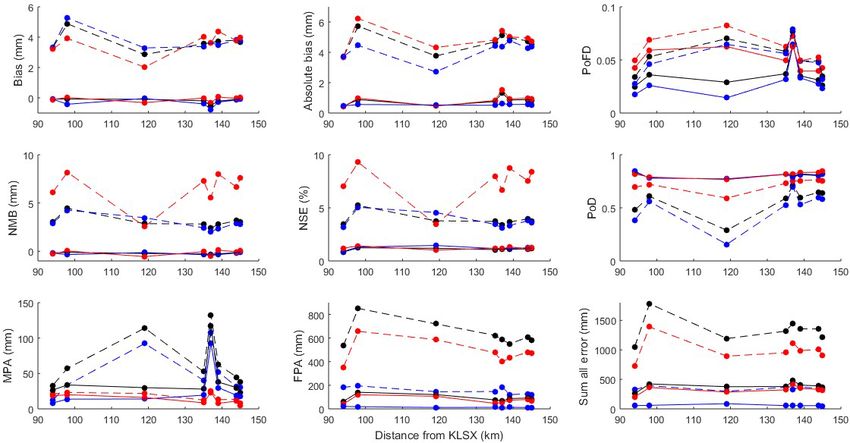
3376                                      M. J. Simpson and N. I. Fox: Dual-polarized quantitative precipitation estimation

   Rain-rate retrieval by weather radars is an estimation           sification algorithm was also tested for performance in cor-
based upon the dielectric properties of the hydrometeors en-        rectly identifying the suitable rain-rate algorithm to choose
countered in the atmosphere. Therefore, there is no direct          based on the Z, ZDR, and KDP radar fields. The current
measurement of rainfall, and this inherently introduces er-         work expands upon that of Simpson et al. (2016) such that
ror. However, dual-polarized radar technology allows for in-        a larger sample of data was analyzed (over 300 h of rainfall
depth analyses on the microphysics of precipitation that sin-       data from 46 separate days in 2014) to encompass multiple
gle polarization was incapable of conducting. In spite of this      different precipitation regimes for both summer and winter,
technology, conflicting studies report the benefits for quan-       with several ground-truth tipping buckets to analyze the per-
titative precipitation estimation (QPE). For example, Gour-         formance of three separate radars as a function of range, and
ley et al. (2010) and Cunha et al. (2015) reported that con-        further expanding upon the effects of erroneous precipitation
ventional R(Z) algorithms have significantly better bias than       estimates on the overall radar error. Objectives for this study
algorithms containing ZDR and/or KDP, while others (e.g.,           included the following: (1) statistically analyze the perfor-
Ryzhkov et al., 2013; Simpson et al., 2016) report the oppo-        mance of each radar at various ranges (compared against the
site. This could be due, at least in part, to the fact that hy-     gauges); (2) compute (a) the amount of precipitation incor-
drometeor types (e.g., rain versus hail) vary on spatial scales     rectly estimated by the radar (quantifying the probability of
that cannot be easily resolved by even densely gauged net-          false detection, PoFD) and (b) the amount of precipitation in-
works.                                                              correctly missed by the radar but measured by the rain gauge;
   Multiple studies have found that the performance of radar        (3) test the overall best radar rain-rate algorithm; and (4) per-
rain-rate estimates decreases as range increases (Smith et al.,     form objectives (1), (2), and (3) while the data are separated
1996; Ryzhkov et al., 2003), which is caused, primarily, by         into warm and cool seasons, which have been shown to result
degradation of beam quality with range. Furthermore, the re-        in significantly different QPEs (Smith et al., 1996; Ryzhkov
searchers also discuss how the probability of detection (PoD)       et al., 2003; Cunha et al., 2015).
at larger ranges decreases, as the radar beam overshoots shal-
low, stratiform precipitation, especially winter precipitation
(Kumjian, 2013b). Bright-banding can also play a crucial            2     Study area and methods
role in significantly increasing the amount of precipitation es-
timated by the radar, prompting many researchers to produce         2.1    Study area
automated bright-band detection algorithms (e.g., Zhang et
al., 2008; Zhang and Qi, 2010).                                     National Weather Service radars from St. Louis (KLSX),
   Despite these overall disadvantages, studies have shown          Kansas City (KEAX), and Springfield (KSGF), MO, are able
that radar rain-rate algorithms seldom exceed absolute er-          to scan the majority of the state of Missouri. Because of this,
rors on the order of 10 mm h−1 (Berne and Uijlenhoet, 2013).        the three aforementioned radars were used to assess overall
However, many of these studies have looked at a small sam-          performance in estimating precipitation for this study. Each
ple of rain events (on the order of 10–50 h) (Kitchen and           radar covered a 200 km radius for which a different num-
Jackson, 1993; Smith et al., 1996; Ryzhkov et al., 2003;            ber of gauges were within their domains: KLSX, KEAX, and
Gourley et al., 2010; Cunha et al., 2013). Long-term per-           KSGF covered 9, 8, and 5 gauges, respectively (Fig. 1).
formances of weather radar are becoming more common in                 Missouri is characterized as a continental type of climate,
recent years as the availability of data becomes more abun-         marked by relatively strong seasonality. Furthermore, Mis-
dant (e.g., Haylock et al., 2008; Goudenhoofdt and Delobbe,         souri is subject to frequent changes in temperature, primar-
2012, 2016; Fairman et al., 2012). Additionally, few studies        ily due to its inland location and its lack of proximity to
(e.g., Smith et al., 1996; Cunha et al., 2015; Simpson et al.,      any large lakes. All of Missouri experiences below-freezing
2016) quantified QPE errors including the probability of de-        temperatures on a yearly basis. For example, the majority
tection and false alarm ratio. In order to gain a better under-     of the state typically registers 110 days with temperatures
standing of the performance of weather radars on rain-rate          below freezing, while the Bootheel (i.e., southeast region)
estimates, more data must be collected over a broad range of        records, on average, 70 days of below-freezing day tempera-
precipitation regimes in addition to an overall broader region      tures, emphasizing the typical northwest to southeast warm-
of interest.                                                        ing pattern of temperatures observed in the state. Because of
   The overarching objective of the current study was to as-        the large variability in temperature, the warm and cool sea-
sess the performance of three different radars within the state     sons were defined from an agronomic perspective, primar-
of Missouri at various ranges from the radar, using terrestrial-    ily taking probabilities of freezing into account. Based on
based tipping bucket gauges as ground-truth data. Radar rain-       the climatological averages of Missouri, from 1983 to 2013,
rate estimation algorithms include 55 algorithms encompass-         November through April registered average minimum tem-
ing standard R(Z) relations as well as algorithms containing        peratures below freezing, which was considered the cool sea-
dual-polarization variables including differential reflectivity     son, while May through October’s minimum average temper-
and the specific differential phase shift. A rain-rate echo clas-   atures were above freezing and constituted the warm season.

Hydrol. Earth Syst. Sci., 22, 3375–3389, 2018                                     www.hydrol-earth-syst-sci.net/22/3375/2018/
M. J. Simpson and N. I. Fox: Dual-polarized quantitative precipitation estimation                                                3377

                                                                       collected using Campbell Scientific TE525 tipping buckets
                                                                       located at each of the locations for the study (Table 1). The
                                                                       precipitation gauges have a 15.4 cm orifice which funnels to a
                                                                       fulcrum which registers 0.254 mm of rainfall per tip. For the
                                                                       current study, none of the day’s average temperature values
                                                                       fell outside of the gauge’s maximum performance range of
                                                                       0 to 50 ◦ C. Accuracy in gauge measurements range between
                                                                       −1 and 1, −3 and 0, and −5 and 0 % for precipitation up
                                                                       to 25.4, 25.4 to 50.8, and 50.8 to 76.2 mm h−1 , respectively,
                                                                       which are, primarily, associated with local random errors and
                                                                       errors in tip-counting schemes (Kitchen and Blackall, 1992;
                                                                       Habib et al., 2001).
                                                                          Each tipping bucket is located, approximately, 1 m above
                                                                       the ground in areas clear of buildings and properly main-
                                                                       tained vegetation height to mitigate turbulence effects (Habib
                                                                       et al., 1999). Due to the well-maintained nature of the
                                                                       mesonet gauges, these errors were assumed negligible and,
                                                                       therefore, allowed for the gauges to be representative of the
Figure 1. Study location (Missouri) with St. Louis (KLSX), Kansas      true rainfall rate. In spite of the non-homogeneous spacing
City (KEAX), and Springfield (KSGF), MO, radars (triangles)            of the gauges, unbiased statistics including the normalized
overlaid with 50, 100, and 150 km range rings in addition to the       mean bias (NMB) and normalized standard error (NSE) were
15 terrestrial-based precipitation gauges utilized as ground-truthed
                                                                       utilized.
data.

                                                                       2.3   Radar data and radar rainfall algorithms
2.2   Rainfall data
                                                                       Next Generation Radar level-II data were retrieved from the
In order for the results to be comparable across the domains           NCDC’s HDSS. Files were processed using the Warning De-
of the three radars it was necessary to select days on which           cision Support System – Integrated Information (WDSS-II)
rain was observed widely across the state. Although mea-               program (Lakshmanan et al., 2007a) to assess reflectivity
surable rainfall occurs on more than 100 days of the year              (Z) in addition to dual-polarized radar variables including
in Missouri with only 50 days typically recording greater              differential reflectivity and specific differential phase shift.
than 0.254 mm, 2014 recorded 46 days with measurable rain-             Three other variables were also generated based on a KDP-
fall throughout the state. Furthermore, occurrence of rain             based smoothing field (Ryzhkov et al., 2003) for reflectiv-
was defined as the observation of an amount greater than               ity, differential reflectivity, and specific differential phase:
0.5 mm (equivalent to two rain gauge tips) in an hour. This            DSMZ, DZDR, and DKDP, respectively. These were imple-
amounted to a total of approximately 300 h of rain across              mented to determine whether the additional KDP-smoothing
those 46 days. This represents a relatively standard year of           fields tend to over- or underestimate QPEs (Simpson et al.,
rainfall for the state of Missouri. Furthermore, the days were         2016). A rain-rate echo classification variable (RREC) was
chosen based on availability of data from the National Cli-            also computed, which chooses whether an R(Z), R(KDP),
mate Data Center’s (NCDC) Hierarchal Data Storage Sys-                 R(Z,ZDR), or R(ZDR, KDP) algorithm is implemented in
tem (HDSS) for all three radars, in addition to error-free             estimating rain rates based on the radar fields of Z, ZDR, and
performance notes from each of the gauges used. The dates              KDP (Kessinger et al., 2003) to determine whether a multi-
analyzed were split near evenly between the warm (May–                 parameter algorithm is superior to a single algorithm.
October) and cool (November–April) seasons, therefore en-                 All seven variables (Z, ZDR, KDP, DSMZ, DZDR,
compassing an overall performance of each of the radars                DKDP, and RREC) were converted from their native polar
throughout the year with no preferential bias towards rain             grid to 256 × 256 1 km Cartesian grids, where the lowest
or snow. Additionally, days were distributed evenly during             radar elevation scans (0.5◦ ) were used to mitigate uncalcu-
the summer between convective and stratiform events with a             lated effects from evaporation and wind drift (Ciach, 2002).
threshold of 38 dBZ (Gamache and Houze, 1982).                         An average of 5 min scans were used for each of the vari-
   Terrestrial-based precipitation gauge data were collected           ables, which were aggregated to hourly totals to be compared
from 15 separate weather stations within the Missouri                  to the hourly tipping-bucket accumulations. In spite of pre-
Mesonet, established by the Commercial Agriculture Pro-                vious reports suggesting 5 min to hourly aggregates can have
gram of University Extension (Table 1). All precipitation              significant effects on QPE (e.g., Fabry et al., 1994), Shuck-
data were aggregated in hourly intervals to match the tempo-           smith et al.’s (2011) criterion of present accumulation ex-
ral resolution of the gauges. Observed precipitation data were         ceeding 26 % for a pixel size of 1 km was not reached.

www.hydrol-earth-syst-sci.net/22/3375/2018/                                         Hydrol. Earth Syst. Sci., 22, 3375–3389, 2018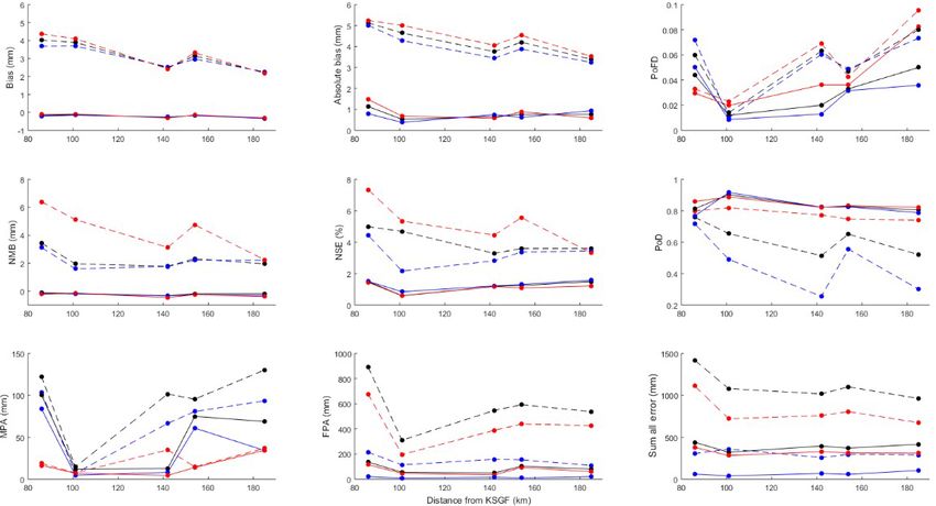
3378                                        M. J. Simpson and N. I. Fox: Dual-polarized quantitative precipitation estimation

Table 1. Terrestrial-based precipitation gauge locations used for the study in addition to the National Weather Service radars from Springfield,
MO (KSGF), Kansas City, MO (KEAX), and St. Louis, MO (KLSX), used in conjunction with each gauge.

                                    Gauge location     Latitude (◦ N)    Longitude (◦ W)       Radar(s) used
                                    Bradford              38.897236          −92.218070        KLSX, KEAX
                                    Brunswick             39.412667          −93.196500        KEAX
                                    Capen Park            38.929237          −92.321297        KLSX, KEAX
                                    Cook Station          37.797945          −91.429645        KLSX, KSGF
                                    Green Ridge           38.621147          −93.416652        KEAX, KSGF
                                    Jefferson Farm        38.906992          −92.269976        KLSX, KEAX
                                    Lamar                 37.493366          −94.318185        KSGF
                                    Linneus               39.856919          −93.149726        KEAX
                                    Monroe City           39.635314          −91.725370        KLSX
                                    Mountain Grove        37.153865          −92.268831        KSGF
                                    Sanborn Field         38.942301          −92.320395        KLSX, KEAX
                                    St. Joseph            39.757821          −94.794567        KEAX
                                    Vandalia              39.302300          −91.513000        KLSX
                                    Versailles            38.434700          −92.853733        KEAX, KSGF
                                    Williamsburg          38.907350          −91.734210        KLSX

Table 2. List of single- and dual-polarimetric algorithms used for radar rainfall estimates.

                               R(Z) = aZ b
                               Precipitation type                                          a         b         c
                               Stratiform                                                200       1.6         –
                               Convective                                                300       1.4         –
                               Tropical                                                  250       1.2         –
                               R(KDP) = a|KDP|b sign(KDP)
                               Algorithm number
                               1                                                        50.7      0.85         –
                               2                                                        54.3      0.81         –
                               3                                                        51.6      0.71         –
                               4                                                         44       0.82         –
                               5                                                        50.3      0.81         –
                               6                                                        47.3      0.79         –
                               R(Z, ZDR) = aZ b ZDRc
                               Algorithm number
                               7                                                6.70 × 10⁻³      0.927    −3.43
                               8                                                7.46 × 10⁻³      0.945    −4.76
                               9                                                1.42 × 10⁻²       0.77    −1.67
                               10                                               1.59 × 10⁻²      0.737    −1.03
                               11                                               1.44 × 10⁻²      0.761    −1.51
                               R(ZDR, KDP) = a|KDP|b ZDRc sign(KDP)
                               Algorithm number
                               12                                                       90.8      0.93    −1.69
                               13                                                        136     0.968    −2.86
                               14                                                       52.9     0.852     -0.53
                               15                                                       63.3     0.851    −0.72

Hydrol. Earth Syst. Sci., 22, 3375–3389, 2018                                             www.hydrol-earth-syst-sci.net/22/3375/2018/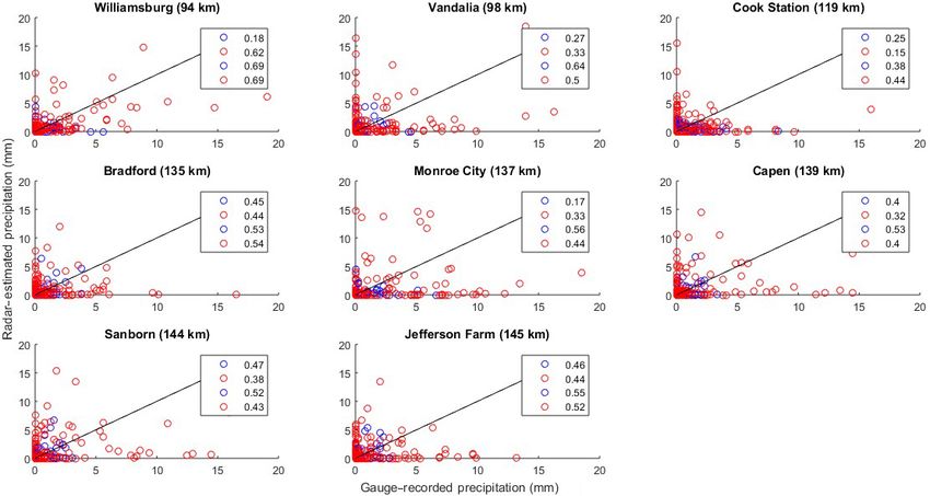
M. J. Simpson and N. I. Fox: Dual-polarized quantitative precipitation estimation                                             3379

   The latitude and longitude of each of the 15 gauges were          the overall results (Chai and Draxler, 2014). Bias measure-
matched with the radar pixel that corresponds to the Carte-          ments (Bias and NMB) were calculated to determine whether
sian grid value of the seven radar variables which were then         radar-derived rain rates were over- or underestimated in com-
implemented in rain-rate calculations. These rain-rate cal-          parison to the gauges. However, to calculate the overall mag-
culations were calculated using the equations presented by           nitude of error associated with the performance of the radars,
Ryzhkov et al. (2005) (Table 2), which were gathered from            the absolute values of Eqs. (1) and (2) were performed to
multiple studies using disdrometers to derive a relationship         yield the mean absolute error and normalized standard error,
between reflectivity, differential reflectivity, and specific dif-   respectively.
ferential phase (Bringi and Chandrasekar, 2001; Brandes et              Several other meteorological parameters were calculated,
al., 2002; Illingworth and Blackman, 2002; Ryzhkov et al.,           including the probability of detection (PoD), which was cal-
2003). Standard R(Z) algorithms were also included to test           culated as
whether the addition of dual-polarized technology improves                   P
                                                                                |Ri · Gi > 0 & Ri > 0|
QPEs.                                                                PoD =             P                ,                       (3)
   With the use of both (i) Z, ZDR, and KDP and (ii) DSMZ,                                |Gi |
DZDR, and DKDP fields produced by WDSS-II, the num-                  where the bullet (·) indicates “if”, to determine how accurate
ber of algorithms tested was 55. This includes the three             the radars were at correctly detecting precipitation. The prob-
standard single-polarized algorithms (stratiform, convective,        ability of detection values range between 0.0 (radar did not
and tropical) which were calculated using reflectivity R(Z)          detect any precipitation correctly) and 1.0 (radar detected the
and then calculated as R(DSMZ), while algorithms 1–6                 occurrence of all precipitation 100 % correctly). The proba-
(R(KDP)) were also calculated as R(DKDP). Algorithms                 bility of false detection (PoFD) takes into account the amount
7–11 (R(Z, ZDR)) were additionally calculated as R(Z,                of precipitation the radars incorrectly estimated when the
DZDR), R(DSMZ, ZDR), and R(DSMZ, DZDR), while the                    gauges recorded zero values, and it was calculated as
same four combinations of non- and KDP-smoothed fields                          P
were applied to the R(KDP, ZDR) algorithms (12–15). Qual-                          Ri · (Gi = 0 & Ri > 0)
                                                                     PoFD =                P                .                    (4)
ity controlling methods for the algorithms include mitigation                                 Gi
of clutter, sun spikes, beam blockage, anomalous propaga-
tion, and removal of non-precipitation echoes (including bi-         Quantitative measures including the missed precipitation
ological and chaff returns) through w2qcnn the w2qcnndp              amount (MPA) and the false precipitation amount (FPA)
algorithms (Lakshmanan et al., 2007b, 2010, 2014).                   were defined such that
                                                                             X
                                                                     MPA =       Ri · (Gi > 0 & Ri = 0),                  (5)
2.4   Statistical analyses                                                  X
                                                                     FPA =      Ri · (Gi = 0 & Ri > 0),                   (6)
To test the performance of each algorithm, several statistical
analyses were calculated. The average difference (Bias) was          which analyzes the total amount of precipitation due to
calculated as                                                        misses and false alarms. The total precipitation error was also
         P                                                           recorded to assess the overall error from each radar.
           (Ri − Gi )
Bias =                ,                                    (1)
              N
                                                                     3     Results and discussion
where Ri is each hourly aggregated radar-estimated rainfall
amount calculated from one of the 55 algorithms, Gi is the           3.1    Overall algorithm performance
hourly aggregated gauge (observed) measurement, and N is
the total number of observations which, for this study, was          To test the overall performance of each radar, it was neces-
300 h. A second statistical parameter, the normalized mean           sary to determine the overall best algorithm for each statisti-
bias (NMB), was calculated as                                        cal measure. The best algorithm from each grouping of equa-
            P                                                        tions was determined to have the lowest normalized standard
          1 (Ri − Gi )                                               error, indicating the best performance relative to the gauge-
NMB =         P          .                               (2)         recorded precipitation amount (Ryzhkov et al., 2005). This
          N      Gi
                                                                     reduces the impact of bias inherent within the dataset be-
The normalized mean bias is included in the analyses due to          tween the warm and cool season, as well as between strat-
the fact that overestimations (i.e., radar estimates larger than     iform and convective events, and allows for statistical mea-
gauge measurements) and underestimations (i.e., radar esti-          surements in spite of the (typical) non-Gaussian behavior of
mates smaller than gauge measurements) are treated propor-           precipitation (Kleiber et al., 2012; Alaya et al., 2017).
tionately. This is directly analogous to choosing the mean ab-          From the results obtained, the three R(Z), three
solute error (MAE) opposed to the standard deviation as the          R(DSMZ), and RREC algorithms displayed a particular
MAE does not penalize smaller or larger errors, obscuring            bias in favor of the R(Z)-convective algorithm for all three

www.hydrol-earth-syst-sci.net/22/3375/2018/                                        Hydrol. Earth Syst. Sci., 22, 3375–3389, 2018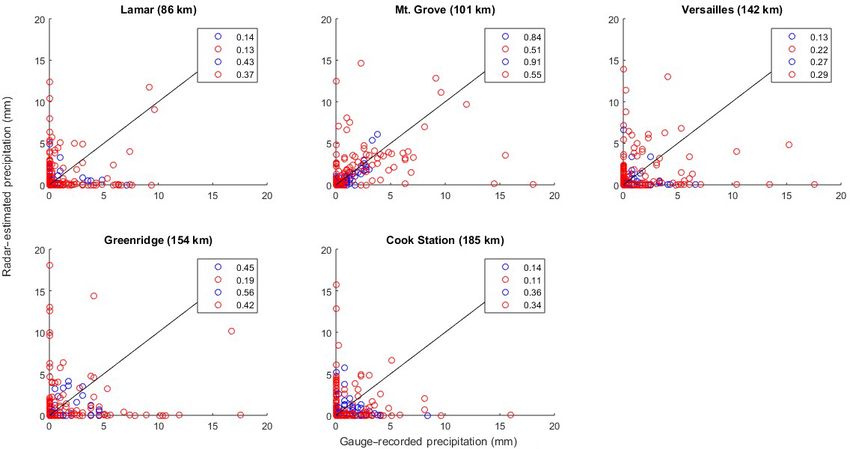
3380                                     M. J. Simpson and N. I. Fox: Dual-polarized quantitative precipitation estimation

Figure 2. Normalized standard error values for the overall performance of the (a) 3 R(Z), 3 R(DSMZ), and RREC algorithms; (b) 6 R(KDP)
and 6 R(DKDP) algorithms (algorithms 1–6 from Table 2); (c) 5 R(Z,ZDR) and 5 R(DSMZ,ZDR) algorithms (Eqs. 7–11 from Table 2); and
(d) 4 R(ZDR,KDP) and 4 R(ZDR,DKDP) algorithms (Eqs. 12–15 from Table 2) for the three radars utilized for the current study.

Hydrol. Earth Syst. Sci., 22, 3375–3389, 2018                                      www.hydrol-earth-syst-sci.net/22/3375/2018/
M. J. Simpson and N. I. Fox: Dual-polarized quantitative precipitation estimation                                                3381

radars with R(Z)-stratiform displaying similar performance           exceeding six units for the second gauge analyzed by KEAX.
(Fig. 2a). This could be due, at least in part, to the near-equal    Algorithms containing DKDP measurements performed bet-
stratiform and convective precipitation regimes throughout           ter than simply KDP, demonstrating that, even with the scal-
2014. Although errors generally increased as range increased         ing behavior of ZDR, DKDP is superior to KDP estimates.
for KEAX and KLSX, the results were nebulous for KSGF.               This provides a potential solution to the noisiness that tends
The lowest NSE values were, typically, closest to each of the        to be exhibited in the KDP field (Ruzanski and Chandrasekar,
radars (between 0.4 and 0.8), with the notable exception of          2012).
the closest gauge to KSGF. In general, the RREC performed               Due to the overall NSE values obtained, for the remain-
worst at the largest of ranges, potentially due to the algo-         der of the analyses, Eq. (11) (i.e., R(Z,ZDR)5) and Eq. (13)
rithm’s ability to incorrectly assess the hydrometeors present       (i.e., R(ZDR,KDP)2) will be utilized as the best and worst
(Cifelli et al., 2010; Yang et al., 2016). Additionally, the poor    algorithms, respectively. Equations containing DZDR were
performance by the R(DSMZ)-tropical equation is due to the           not included in the following discussion due to the very large
lack of tropical precipitation within central Missouri. Over-        QPE errors for each radar.
all, the KDP-smoothed reflectivity fields (DSMZ) performed
worse than their counterparts, resulting in over-prediction of
                                                                     3.2   KEAX
precipitation and, thus, larger errors (Simpson et al., 2016).
Errors did not exceed 2.4 NSE units for any of these algo-
rithms.                                                              The overall bias showed that there was a positive bias, peak-
   However, the performance of the KDP-smoothed KDP                  ing near 5.5 mm h−1 at the second gauge for KEAX, approx-
field (DKDP) performed better than the original specific dif-        imately 115 km from the radar for both the best- and worst-
ferential phase shift field (Fig. 2b). For nearly all gauges for     performing algorithms (Fig. 3). This corresponds well with
each of the three radars, R(DKDP)4 performed the best, with          the spike in the falsely detected precipitation recorded, which
NSE values ranging from 1.4 to 4.1. The range of NSE values          is canceled by the maximum in missed precipitation at the
were largest at KEAX, while the spread was relatively small          second distance of, approximately, 150 km. The overall worst
for KLSX and KSGF. In spite of this, the overall spread of the       algorithm, Eq. (13), an R(ZDR,KDP) relationship, revealed
performance of the 12 KDP algorithms varied greatly (aver-           a decreasing trend in bias as the distance from the radar in-
age of 2 NSE units), exhibiting the sensitivity of KDP esti-         creased. For example, a bias of 4 mm h−1 was observed at a
mates on QPE (Ryzhkov et al., 2005; Cunha et al., 2013). In          distance of 75 km from the radar, whereas the bias reduced
general, the NSSL-derived R(KDP) equations (i.e., Eqs. 4–            to 3 mm h−1 at distances near 175 km. This could be due, at
6) outperformed those from Bringi and Chandrasekar (2001,            least in part, to the algorithm’s utilization of KDP, which per-
Eq. 1), Brandes et al. (2002, Eq. 2), and Illingworth and            forms poorly in frozen (especially light) precipitation (Zrnic
Blackman (2002, Eq. 3). Regardless, the magnitudes were              and Ryzhkov, 1996; Kumjian, 2013a), causing the overesti-
all, approximately, more than 1 NSE unit than the perfor-            mation. Conversely, the algorithm with the lowest bias was
mance of the R(Z) algorithms.                                        an R(Z,ZDR) algorithm (Eq. 11). There was a maximum in
   The algorithms with the lowest NSE values were Eqs. (7)–          the bias calculations while utilizing Eq. (11) near 120 km,
(11). For example, the overall lowest NSE was at a distance          similar to Eq. (13); however, there was a more pronounced
of 130 km from KEAX (0.3), with no locations exceeding               minimum in the data near 150 km. Furthermore, it appears
NSE values of 2.0 (Fig. 2c). The large values at the clos-           the data oscillates around a bias value of 0 mm h−1 when us-
est location for KSGF (85 km, 1.3–1.9 NSE units) and the             ing Eq. (13). This could be due to ZDR’s capability to re-
fifth closest gauge to KLSX (135 km, 1.3–1.8 NSE units),             spond to precipitation shape (Kumjian, 2013a), which helps
Cook Station, were similar to the R(Z) and R(DSMZ) re-               to scale the reflectivity portion of the rainfall estimation algo-
sults, indicating potential issues with reflectivity measure-        rithm to a more accurate value (Seo et al., 2015). In general,
ments. Additionally, these locations were the closest in per-        the cool season displayed a larger magnitude of error in terms
formance to the R(KDP) and R(DKDP) NSE values. Ob-                   of bias for both algorithms.
servations from this gauge (Cook Station) indicated hail oc-            The normalized mean bias reveals the same trend in val-
curred during the evening of 1 August, for which KDP esti-           ues for bias but with an overall decrease in magnitude. It is
mates would be more ideal than Z for QPE (Ryzhkov et al.,            important to note, however, that the algorithms that tend to
2005; Kumjian, 2013a; Cunha et al., 2015). In spite of this,         perform the worst (e.g., algorithms containing KDP) result
the overall spread in performance of the R(Z,ZDR) equa-              in anomalous range responses which would be due, at least
tions was lower than the R(KDP) equations, demonstrating             in part, to a stronger response to precipitation type (Kumjian,
the robust performance of R(Z,ZDR) for QPE (Wang and                 2013c). This indicates that observations above the melting
Chandrasekar, 2010; Seo et al., 2015).                               layer are dominant, for which QPEs tend not to be calculated
   The R(ZDR,KDP) algorithms performed the worst, over-              (Cifelli et al., 2011; Seo et al., 2015), but are important for
all (Fig. 2d). In spite of the differential reflectivity being im-   regions devoid of adequate radar coverage (Ryzhkov et al.,
plemented, the overall NSE values increased in magnitude,            2003; Simpson et al., 2016).

www.hydrol-earth-syst-sci.net/22/3375/2018/                                       Hydrol. Earth Syst. Sci., 22, 3375–3389, 2018
3382 M. J. Simpson and N. I. Fox: Dual-polarized quantitative precipitation estimation Figure 3. Values of analyses from the Kansas City radar. Dashed lines and points represent the analyses of the worst-performing algorithm (R(ZDR,KDP)), while the solid lines and points represent the analyses of the best-performing algorithm (R(Z,ZDR)). Red, blue, and black colors represent analyses conducted during the warm season, cool season, and overall, respectively. Figure 4. Correlation coefficient values for the nine locations analyzed by the Kansas City radar with the R(Z,ZDR) NSSL equation. Blue and red scatter points represent the cool and warm season data, respectively. The top two numbers on each plot indicate the overall R 2 value, whereas the bottom two numbers represent the R 2 when false alarms and misses are removed. The absolute bias and normalized standard error shows the gauge at, approximately, 150 km (Linneus) with values of same maxima in the data at the second gauge (Brunswick) 5.9 mm h−1 and 4.0, respectively. Bright-band issues are de- that was present in the bias data (6.2 mm h−1 and 5.6, re- tected due, at least in part, to the increased missed precip- spectively). However, a second maxima is located at the fifth itation amount (240 mm) at this particular distance for the Hydrol. Earth Syst. Sci., 22, 3375–3389, 2018 www.hydrol-earth-syst-sci.net/22/3375/2018/
M. J. Simpson and N. I. Fox: Dual-polarized quantitative precipitation estimation 3383
R(ZDR,KDP) equation (i.e., worst-performing algorithm). NMB data. Additionally, the overall trend of decreasing bias
There was also a pronounced minimum in the absolute bias and NMB as distance from the radar increases was noted,
and NSE results at the fourth gauge for equations 11 and 13, presumably due to overshooting effects similar to the KEAX
4.0 and 0.8 mm h−1 , and 2.8 and 0.8, respectively, potentially data. Furthermore, the overall non-biased results from the
indicating an idealized range of QPE for KEAX. Further- R(Z,ZDR) equation demonstrates its robust capabilities in
more, the historical records at this particular gauge showed QPE, in spite of its sensitivity to calibration (Zrnic et al.,
less issues (e.g., clogging) than any of the others analyzed by 2005; Bechini et al., 2009; Gorgucci et al., 1992).
the KEAX radar. This highlights the importance of choos- The double maxima in the absolute bias graph are present
ing ground-truth data, in particular tipping buckets which are as with the KEAX data, but are not as pronounced. For ex-
prone to numerous errors (Ciach and Krajewski, 1999b).The ample, the absolute biases at 95 and 140 km from KLSX
largest contributions to the NSE and NMB were due to the were 5.9 and 4.9 mm for Eq. 13, while the values were 1.1
warm season. and 1.4 mm for Eq. 11, accordingly. Additionally, the overall
The probability of detection results indicate a large dif- minima in the absolute bias for both KEAX and KLSX are at,
ference in algorithm choice for correctly detecting precip- approximately, 125 km from the radar (3.9 and 1.0 mm h−1 ,
itation. The low PoD at, approximately 150 km, indicates respectively, for Eqs. 13 and 11). The relative distance from
overshooting of the beam. This is further evidenced by the the radars are the same, where the two maxima for KEAX
MPA results, as about 225 mm of precipitation was missed were at 115 and 150 km, while the maxima were at, ap-
by the radar at 150 km, whereas only 100 mm of precipita- proximately, 100 and 140 km for KLSX. The overall best-
tion was missed by the radar at the second gauge at 120 km. and worst-performing algorithms at KLSX for the absolute
Although Eq. (11), an R(Z,ZDR) algorithm, was superior in bias and NSE were Eqs. (11) and (13), the R(Z,ZDR) and
terms of the bias, the same algorithm with a KDP-smoothed R(ZDR,KDP) algorithms, respectively.
reflectivity value, R(DSMZ,ZDR), revealed the overall least The magnitude of error in terms of absolute bias, normal-
amount of the falsely missed precipitation (by 10 mm). How- ized mean bias, and normalized standard error all showed a
ever, the summation of the amount of precipitation falsely decreasing pattern as distance from KLSX increased. This
detected (PoFD) by KEAX showed a larger source of error was due, primarily, from a maximum in the false precipita-
than the MPA in terms of magnitude. For example, at the tion amount at 95 km from the radar. Historical notes at this
second (fifth) gauge, only 100 (225) mm of precipitation was location indicate frequent clogging of the rain gauge, either
missed by the radar, but over 700 (725) mm of precipitation due to bugs or leaves. From a particular series of events span-
was incorrectly estimated by the radar. ning from 1 to 4 April and 1 to 3 August 2014, over 130 mm
Correlation coefficient (CC) values for any of the nine sta- of precipitation occurred during each period which was not
tions analyzed by KEAX range from 0.02 (Linneus, 151 km) captured by the gauge, resulting in a large amount of overall
to 0.93 for the cool season (St. Joseph, 115 km). The low- error. These results indicate the importance of dual gauges in
est R 2 values were due to a combination of false alarms and the same vicinity (Krajewski et al., 1998; Ciach and Krajew-
misses. For example, the CC values for the warm seasons ski, 1999a). Interestingly, the cool season displayed a larger
at Sanborn (170 km) and Jefferson Farm (173 km) were 0.22 NSE (5 % for R(ZDR,KDP)) potentially due to the very low
and 0.24, respectively, whereas when the instances of false probability of detection (0.2) at this range of 118 km.
alarms and misses were removed the CC values increased One of the main differences between the KLSX and
to 0.48 and 0.52. Few locations (Brunswick, 114 km; and KEAX data was the decreased probability of detection at
Versailles, 129 km) saw little improvement in the CC values 120 km for KLSX, while there was an increased probabil-
when only hits were analyzed (less than 0.1 increase), indi- ity of detection for KEAX. In general, the PoD values were
cating the mean absolute error (in terms of hits) contributed worse for KLSX when compared to KEAX. For example,
the largest portion of error. Eq. (11) had no PoD values below 0.90, whereas no PoD val-
ues exceeded 0.84 for KLSX. There was also a slight trend
3.3 KLSX of increasing PoD values as distance from the St. Louis radar
increased and, at one point near 140 km, the best algorithm,
Unlike the KEAX data, the gauges used for analyses for the R(DSMZ)-convective, and the worst algorithm, KDP1, were
KLSX radar span between 90 and 150 km. Furthermore, five not significantly different (p < 0.10). Additionally, the max-
out of the eight gauges were located within a 10 km of range ima in the PoD while utilizing KDP1 correspond to a minima
from one another, near 140 km from the radar, limiting the in the R(DSMZ) detection percentage, which is well corre-
data available for analyses between 100 and 140 km (Fig. 5). lated by the similarly valued MPA results.
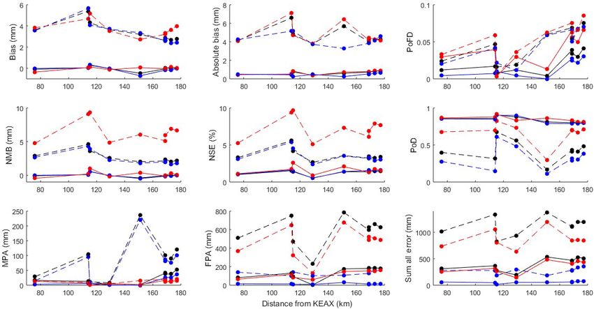
The bias and NMB both show a relatively modest peak The missed precipitation amount (MPA) showed that the
in values near the second gauge of 5 mm, which decreases cool season contributed the most, whereas the warm sea-
to approximately 3.6 mm at the third gauge, 120 km from son contributed the most amount of the false precipitation
the radar. The worst-performing algorithm, Eq. (13), had the amount. The R(Z,ZDR) equation only registered, on av-
same R(ZDR,KDP) relation as the worst KEAX bias and erage, 25 mm of MPA and 160 mm of FPA, whereas the
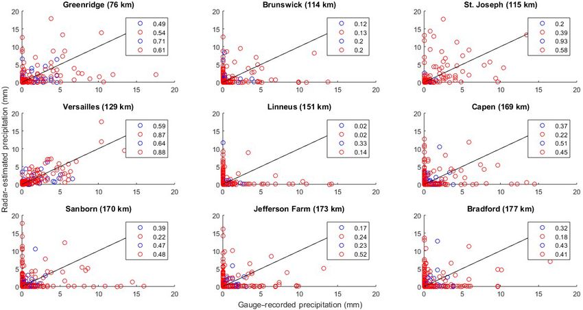
www.hydrol-earth-syst-sci.net/22/3375/2018/ Hydrol. Earth Syst. Sci., 22, 3375–3389, 20183384 M. J. Simpson and N. I. Fox: Dual-polarized quantitative precipitation estimation Figure 5. Values of analyses from the St. Louis radar. Dashed lines and points represent the analyses of the worst-performing algorithm (R(ZDR,KDP)), while the solid lines and points represent the analyses of the best-performing algorithm (R(Z,ZDR)). Red, blue, and black colors represent analyses conducted during the warm season, cool season, and overall, respectively. Figure 6. Correlation coefficient values for the eight locations analyzed by the St. Louis radar with the R(Z,ZDR) NSSL equation. Blue and red scatter points represent the cool and warm season data, respectively. The top two numbers on each plot indicate the overall R 2 value, whereas the bottom two numbers represent the R 2 when false alarms and misses are removed. R(ZDR,KDP) equation was very dependent upon range. For from KLSX) displayed a sharp increase in the MPA for both example, the FPA from R(ZDR,KDP) decreased as range in- cool seasons (above 100 mm). creased from the radar from a maximum of, approximately, 850 to 620 mm. However, the fifth-furthest gauge (137 km Hydrol. Earth Syst. Sci., 22, 3375–3389, 2018 www.hydrol-earth-syst-sci.net/22/3375/2018/
M. J. Simpson and N. I. Fox: Dual-polarized quantitative precipitation estimation                                                  3385

Figure 7. Values of analyses from the Springfield radar. Dashed lines and points represent the analyses of the worst-performing algorithm
(R(ZDR,KDP)), while the solid lines and points represent the analyses of the best-performing algorithm (R(Z,ZDR)). Red, blue, and black
colors represent analyses conducted during the warm season, cool season, and overall, respectively.

3.4   KSGF                                                             error magnitude as range increased. In spite of this, the PoFD
                                                                       results indicate both algorithms increased in PoFD values as
                                                                       range increased, with the warm season typically dominating,
In spite of the fact that the KLSX and KEAX data strongly              particularly due to the large convective clouds dominating in
suggest false precipitation errors near 100 km in addition to          the warm season. False detection values as low as 0.01 for
bright-banding near 150 km from the radars, the KSGF re-               the cool season while utilizing R(Z,ZDR) were observed at
sults reveal an overall smooth decrease (increase) of error            distances near 100 and 140 km from the radar.
with range (Fig. 7) for R(ZDR,KDP) and R(Z,ZDR), ac-                      Normalized standard error values increased from 0.7 % at
cordingly. One of the main reasons for this could be due to            a distance of 105 km to 1.8 % at a distance of 185 km for
the fact that only five gauges were analyzed from KSGF (the            R(Z,ZDR). Large NSE values for the warm season (7.5 %)
fewest of the three radars analyzed), smoothing the overall            were calculated for R(ZDR,KDP), which decreased to 3.8 %
trend lines.                                                           at 185 km from the radar. Furthermore, this was the only in-
   The bias remained relatively constant near −0.3 mm for              stance when the warm season was less than the cool season
R(Z,ZDR), whereas the bias exhibited a sharp decrease from             in terms of NSE. Otherwise, the overall NSE decreased from
4 to 2.7 mm over a distance of, approximately, 100 km. In              5 to 3.9 % for R(ZDR,KDP). The NMB followed a similar
general, the cool season displayed lower bias magnitudes               trend for the KDP-containing algorithm, with a noticeable
when compared to the warm season, similar to the KEAX                  exception at the second gauge (105 km from KSGF), where
results. This may be due, at least in part, to the low PoFD            the overall NSE was closer to the warm season than the cool
values for the warm season close to the KSGF radar.                    season. This is due to the low PoFD values at this location, in
   Similar to the bias, the absolute bias for R(Z,ZDR)                 addition to a smaller difference between the two algorithm’s
was constant at all ranges (near 1 mm), whereas the                    FPA measurements.
R(ZDR,KDP) equation decreased from 5.2 to 3.8 mm. This                    The MPA results, unlike for KEAX and KLSX, displayed
is potentially due to the low cool season PoD values (below            a larger range of performance between seasons. However,
0.6), while the warm season R(ZDR,KDP) values (near 0.8)               the warm season still exhibited the overall best performance
remained constant. A larger contribution from more correctly           in terms of MPA, yet contributed the most to the FPA for
detected precipitation in addition to the decreasing trends in         both R(Z,ZDR) and R(ZDR,KDP). In spite of the MPA
the NMB and NSE would result in a lower absolute bias.                 typically increasing as range increased, the FPA was more
   The closest location (90 km) typically displayed the largest        nebulous. For example, the second gauge (105 km from
errors for the R(ZDR,KDP) equation and then decreased in

www.hydrol-earth-syst-sci.net/22/3375/2018/                                          Hydrol. Earth Syst. Sci., 22, 3375–3389, 2018
3386 M. J. Simpson and N. I. Fox: Dual-polarized quantitative precipitation estimation
Figure 8. Correlation coefficient values for the five locations analyzed by the Springfield radar with the R(Z,ZDR) NSSL equation. Blue
and red scatter points represent the cool and warm season data, respectively. The top two numbers on each plot indicate the overall R 2 value,
whereas the bottom two numbers represent the R 2 when false alarms and misses are removed.
KSGF) had the overall lowest NSE (0.8 %), MPA (15 mm), 4 Conclusions
and FPA (95 mm) for R(Z,ZDR). The third-furthest loca-
tion (142 km) resulted in slightly larger errors, overall, while Dual-polarization technology was implemented in the Na-
the fourth-furthest location had errors similar to the second tional Weather Service Next Generation Radar network in
gauge (105 km). Then, at the furthest tipping bucket location the spring of 2012 to, primarily, improve quantitative precip-
(185 km), NSE values increased, whereas FPA and MPA de- itation estimation and hydrometeor classification. The cur-
creased. Therefore, the furthest location’s errors are due, pri- rent study observed over 300 h of precipitation data with
marily, from discrepancies between precipitation magnitude three separate radars in Missouri using 55 algorithms includ-
between the gauge and radar. ing the three conventional R(Z) radar rain-rate estimation
Excluding Versailles (142 km from KSGF), the cool sea- algorithms (stratiform, convective, and tropical) along with
son exhibited larger R 2 values in comparison to the cool a myriad of R(KDP), R(Z,ZDR), and R(ZDR,KDP) algo-
season (Fig. 8). Furthermore, CC values exceeded 0.9 when rithms, which can be found in Ryzhkov et al. (2005). Ad-
false alarms and misses were excluded from Mountain Grove ditionally, a KDP-smoothing field of reflectivity, differential
(101 km) and were 0.84 when included. Otherwise, the other reflectivity, and the specific differential phase shift (DSMZ,
four stations analyzed by the Springfield radar displayed DZDR, and DKDP, respectively) were measured and used
many counts of false alarms and misses, leading to low R 2 for analyses. Unlike previous studies, the current work em-
values. phasizes the amount of precipitation correctly and incorrectly
Due to the relatively large ranges from the Springfield estimated by the radar in comparison to the terrestrial-based
radar, most of the correlation coefficient values were low in precipitation gauges through measurements of the missed
comparison to either KLSX or KEAX. For the warm (cool) and false precipitation amount.
season without false alarms and misses, R 2 values ranged For all three radars – Kansas City, St. Louis, and Spring-
from 0.44 (0.38) to 0.34 (0.36) for KLSX and KSGF, respec- field, MO – the majority of precipitation error (over 60 %)
tively, at Cook Station (119 and 185 km). Similarly, the CC was contributed by the amount of precipitation falsely de-
values ranged from 0.61 (0.71) to 0.42 (0.56) at Green Ridge tected by the radar (up to 725 mm), while 20 % was due
(76 and 154 km) for KEAX and KSGF, accordingly. to the radar missing the precipitation (up to 225 mm) for
KEAX. Similar magnitudes of error were reported for KLSX
and KSGF, with an overall error in precipitation for each
radar ranging between 250 mm for the best performing
of the 55 algorithms, Eq. (11) (an R(Z,ZDR) algorithm),
Hydrol. Earth Syst. Sci., 22, 3375–3389, 2018 www.hydrol-earth-syst-sci.net/22/3375/2018/M. J. Simpson and N. I. Fox: Dual-polarized quantitative precipitation estimation 3387
and up to 2000 mm for the worst-performing algorithms, NOAA, 2017) or from the Missouri Mesonet (http://agebb.missouri.
R(ZDR,KDP) Eq. (13). The R(Z,ZDR) equation (an NSSL edu/weather/stations/; AgEBB, 2017).
algorithm) was determined to be the most robust due to it reg-
istering the lowest NSE. These values of false precipitation
amount and missed precipitation amount generally increased Author contributions. NF designed the experiment and provided
as range from the radar increased. feedback while MS carried out the calculations and wrote the
Most algorithms showed a degradation in the normalized manuscript.
standard error with range. In particular, the KDP-smoothed
equations displayed larger biases and NSE values than their
Competing interests. The authors declare that they have no conflict
non-KDP counterparts, with the exception of R(KDP) al-
of interest.
gorithms themselves. Some larger errors were recorded at
gauge locations close to the radar, potentially due to bright-
banding effects which were determined to be due to the large Acknowledgements. This material is based upon work sup-
false precipitation amount analyzed at these locations. ported by the National Science Foundation under award number
The data were divided into summer (May–October) and IIA-1355406. Any opinions, findings, and conclusions or recom-
winter (November–April; 59 and 41 % of the entire data, re- mendations expressed in this material are those of the authors
spectively). Despite the winter data contributing less than and do not necessarily reflect the views of the National Science
the summertime data, they accounted for 20 % of the over- Foundation.
all MPA and 40 % to the overall PoFD. The R 2 values were
lower during the winter in comparison to the warm season, Edited by: Remko Uijlenhoet
primarily due to the smaller magnitude of precipitation that Reviewed by: two anonymous referees
occurred. Furthermore, CC values increased by as much as
0.4 when instances of hits and misses were removed from
the analyses, resulting in the warm season outperforming the References
cool season CC values at particularly short ranges from the
radar. AgEBB (Agricultural Electronic Bulletin Board): Missouri
Mesonet, available at: http://agebb.missouri.edu/weather/
These results aid in our understanding of the possibilities
stations/, last access: February 2017.
for hydrometeorological studies. Nearly 50 % of the 300 h
Alaya, M. A., Ourda, T. B. M. J., and Chebana, F.: Non-
where precipitation occurred analyzed for the study con- Gaussian spatiotemporal simulation of multisite precipita-
sisted of either falsely estimated precipitation by the radar, tion: Downscaling framework, Clim. Dynam., 50, 1–15,
or missed by the radar. Furthermore, these errors accumu- https://doi.org/10.1007/s00382-017-3578-0, 2017.
late between 500 and 2000 mm of precipitation depending Anagnostou, M. N., Anagnostou, E. N., Vulpiani, G., Montopoli,
on the algorithms chosen. Although the overall performance M., Marzano, F. S., and Vivekanandan, J.: Evaluation of X-band
increased when false alarms and misses were removed, corre- polarimetric-radar estimates of drop-size distributions from co-
lation coefficient values still, typically, remained below 0.50 incident S-band polarimetric estimated and measured raindrop
at ranges beyond 130 km. spectra, IEEE T. Geosci. Remote, 46, 3067–3075, 2008.
Furthermore, results demonstrate the issues with analyz- Bechini, R., Baldini, L., Cremonini, R., and Gorgucci, E.: Differ-
ential reflectivity calibration for operational radars, J. Atmos.
ing QPE from a single gauge, explaining why the Commu-
Ocean. Tech., 25, 1542–1555, 2009.
nity Collaborative Rain, Hail, and Snow Network (Kelsch,
Berne, A. and Krajewski, W. F.: Radar for hydrology: Unfulfilled
1998; Cifelli et al., 2005; Reges et al., 2016) or other promise or unrecognized potential?, Adv. Water Resour., 51,
densely gauged networks (e.g., the Hydrometeorological Au- 357–366, 2013.
tomated Data System, HADS; and the Meteorological As- Berne, A. and Uijlenhoet, R.: A stochastic model of range
similation Data Ingest System, MADIS) tend to be more uti- profiles of raindrop size distributions: application to
lized since results have shown that measurements or quality- radar attenuation correction, Geophys. Res. Lett., 32,
controlled techniques made by these organizations, espe- https://doi.org/10.1029/2004GL021899, 2005.
cially CoCoRaHS (Community Collaborative Rain, Hail and Brandes, E. A., Zhang, G., and Vivekanandan, J.: Experiments in
Snow Network), are significantly more accurate than rain rainfall estimation with a polarimetric radar in a subtropical en-
gauges (Simpson et al., 2017), especially for convective vironment, J. Appl. Meteorol., 41, 674–685, 2002.
Brandes, E. A., Zhang, G., and Vivekanandan, J.: Drop size distri-
events (Moon et al., 2009).
bution retrieval with polarimetric radar: model and application,
J. Appl. Meteorol., 43, 461–475, 2004.
Bringi, V. N. and Chandrasekar, V.: Polarimetric Doppler weather
Data availability. All data can be accessed through the Na- radar, principles and applications, Cambridge University Press:
tional Center for Environmental Information’s (NCEI) Hierarchal Cambridge, UK, 636 pp., 2001.
Data Storage System (https://www.ncdc.noaa.gov/has/has.dsselect; Chai, T. and Draxler, R. R.: Root mean square error (RMSE)
or mean absolute error (MAE)? – Arguments against avoid-
www.hydrol-earth-syst-sci.net/22/3375/2018/ Hydrol. Earth Syst. Sci., 22, 3375–3389, 20183388 M. J. Simpson and N. I. Fox: Dual-polarized quantitative precipitation estimation ing RMSE in the literature, Geosci. Model Dev., 7, 1247–1250, Habib, E., Krajewski, W. F., and Kruger, A.: Sampling errors of https://doi.org/10.5194/gmd-7-1247-2014, 2014. tipping-bucket rain gauge measurements, J. Hydrol. Eng., 6, Ciach, G. J. and Krajewski, W. F.: On the estimation of radar rainfall 159–166, 2001. error variance, Adv. Water Resour., 22, 585–595, 1999a. Haylock, M. R., Hofstra, N., Klein Tank, A. M. G., Klok, Ciach, G. J. and Krajewski, W. F.: Radar-raingage comparisons un- E. J., Jones, P. D., and New, M.: A European daily der observational uncertainties, J. Appl. Meteorol., 38, 1519– high-resolution gridded data set of surface temperature 1525, 1999b. and precipitation for 1950–2006, J. Geophys. Res., 113, Ciach, G. J.: Local random errors in tipping-bucket rain gauge mea- https://doi.org/10.1029/2008JD010201, 2008. surements, J. Atmos. Ocean. Tech., 20, 752–759, 2002. Holleman, I., Huuskonen, A., Gill, R., and Tabary, P.: Operational Cifelli, R., Doesken, N., Kennedy, P., Carey, L., Rutledge, S. A., monitoring of radar differential reflectivity using the sun, J. At- Gimmestad, C., and Depue, T.: The community collaborative mos. Ocean. Tech., 27, 881–887, 2010. rain, hail, and snow network: Informal education for scientists Hubbert, J. C.: Differential reflectivity calibration and antenna tem- and citizens, B. Am. Meteorol. Soc., 86, 1069–1077, 2005. perature, J. Atmos. Ocean. Tech., 34, 1885–1906, 2017. Cifelli, R., Chandrasekar, V., Lim, S., Kennedy, P. C., Wang, Y., and Illingworth, A. and Blackman, T. A.: The need to represent raindrop Rutledge, S. A.: A new dual-polarization radar rainfall algorithm: size spectra as normalized gamma distributions for the interpre- Application in Colorado precipitation events, J. Atmos. Ocean. tation of polarization radar observations, J. Appl. Meteorol., 41, Tech., 28, 352–364, 2010. 286–297, 2002. Cunha, L. K., Smith, J. A., Baeck, M. L., and Krajewski, W. F.: Kelsch, M.: The Fort Collins flash flood: Exceptional rainfall and An early performance of the NEXRAD dual-polarization radar urban runoff, Preprints, 19th Conference on severe local storms, rainfall estimates for urban flood applications, Weather Forecast., Minneapolis, MN, American Meteorological Society, 404–407, 28, 1478–1497, 2013. 1998. Cunha, L. K., Smith, J. A., Krajewski, W. F., Baeck, M. L., and Seo, Kessinger, C., Ellis, S., and Van Andel, J.: The radar echo classifier: B.: NEXRAD NWS polarimetric precipitation product evalua- a fuzzy logic algorithm for theWSR-88D, 19th Conf. on Inter. tion for IFloods, J. Hydrometeorol., 16, 1676–1699, 2015. Inf. Proc. Sys. (IIPS) for Meteor., Ocean., and Hydr., Amer. Me- Fabry, F., Bellon, A., Duncan, M. R., and Austin, G. L.: High reso- teor. Soc., Long Beach, CA, 2003. lution rainfall measurements by radar for very small basins: the Kitchen, M. and Blackall, M.: Representativeness errors in com- sampling problem reexamined, J. Hydrol., 161, 415–428, 1994. parisons between radar and gauge measurements of rainfall, J. Fairman, J. G., Schultz, D. M., Kirschbaum, D. J., Gray, Hydrol., 134, 13–33, 1992. S. L., and Barrett, A. I.: A radar-based rainfall climatol- Kitchen, M. and Jackson, P. M.: Weather radar performance at long ogy of Great Britain and Ireland, Weather, 70, 153–158, range – simulated and observed, J. Appl. Meteorol., 32, 975–985, https://doi.org/10.1002/wea.2486, 2012. 1993. Gamache, J. F. and Houze, R. A.: Mesoscale air motions associated Kleiber, W., Katz, R. W., and Rajagopalan, B.: Daily spa- with a tropical squall line, Mon. Weather Rev., 110, 118–135, tiotemporal precipitation simulation using latent and trans- 1982. formed Gaussian processes, Water Resour. Res., 48, W01523, Giangrande, S. E. and Ryzhkov, A. V.: Estimation of rainfall based https://doi.org/10.1029/2011WR011105, 2012. on the results of polarimetric echo classification, J. Appl. Mete- Krajewski, W. F., Kruger, A., and Nespor, V.: Experimental and nu- orol., 47, 2445–2460, 2008. merical studies of small-scale rainfall measurements and vari- Gorgucci, E., Scarchilli, G., and Chandrasekar, V.: Calibration of ability, Water Sci. Technol., 37, 131–138, 1998. radars using polarimetric techniques, IEEE T. Geosci. Remote, Kumjian, M. R.: Principles and applications of dual-poarization 30, 853–858, 1992. weather radar, Part 1: Description of the polarimetric radar vari- Gorgucci, E., Scarschilli, G., Chandrasekar, V., and Bringi, V. N.: ables, Journal of Operational Meteorology, 1, 226–242, 2013a. Measurement of mean raindrop shape from polarimetric radar Kumjian, M. R.: Principles and applications of dual-poarization observations, J. Atmos. Sci., 57, 3406–3413, 2000. weather radar, Part 2: Warm and cold season applications, Jour- Gorgucci, E., Baldini, L., and Chandrasekar, V.: What is the shape nal of Operational Meteorology, 1, 243–264, 2013b. of a raindrop? An answer from radar measurements, J. Atmos. Kumjian, M. R.: Principles and applications of dual-poarization Sci., 63, 3033–3044, 2006. weather radar, Part 3: Artifacts. Journal of Operational Meteo- Goudenhoofdt, E. and Delobbe, L.: Long-term evaluation of radar rology, 1, 265–274, 2013c. QPE using VPR correction and radar-gauge merging, Interna- Lakshmanan, V., Smith, T., Stumpf, G., and Hondl, K.: The warn- tional Association of Hydrological Sciences Publications, 351, ing decision support system – integrated information, Weather 249–254, 2012. Forecast., 22, 596–612, 2007a. Goudenhoofdt, E. and Delobbe, L.: Generation and verification of Lakshmanan, V., Fritz, A., Smith, T., Hondl, K., and Stumpf, G.: rainfall estimates from 10-yr volumetric weather radar measure- An automated technique to quality control radar reflectivity data, ments, J. Hydrometeorol., 133, 1191–1204, 2016. J. Appl. Meteorol. Clim., 46, 288–305, 2007b. Gourley, J. J., Giangrande, S. E., Hong, Y., Flamig, Z., Schuur, T., Lakshmanan, V., Zhang, J., and Howard, K.: A technique to censor and Vrugt, J.: Impacts of polarimetric radar observations on hy- biological echoes in radar reflectivity data. J. Appl. Meteorol. drologic simulation, J. Hydrometeorol., 11, 781–796, 2010. Clim., 49, 453–462, 2010. Habib, E., Krajewski, W. F., Nespor, V., and Kruger, A.: Numeri- Lakshmanan, V., Karstens, C., Krause, J., and Tang, L.: Quality con- cal simulation studies of rain gauge data correction due to wind trol of weather radar data using polarimetric variables, J. Atmos. effect, J. Geophys. Res., 104, 723–734, 1999. Ocean. Tech., 31, 1234–1249, 2014. Hydrol. Earth Syst. Sci., 22, 3375–3389, 2018 www.hydrol-earth-syst-sci.net/22/3375/2018/
You can also read