High Spatial Resolution Remote Sensing for Salt Marsh Mapping and Change Analysis at Fire Island National Seashore - MDPI
←
→
Page content transcription
If your browser does not render page correctly, please read the page content below
remote sensing
Article
High Spatial Resolution Remote Sensing for Salt
Marsh Mapping and Change Analysis at Fire Island
National Seashore
Anthony Campbell 1,2 and Yeqiao Wang 1, *
 1    Department of Natural Resources Science, University of Rhode Island, Kingston, RI 02881, USA;
      anthony.d.campbell@yale.edu
 2    Currently at the Yale School of Forestry & Environmental Studies, New Haven, CT 06511, USA
 *    Correspondence: yqwang@uri.edu

 Received: 3 April 2019; Accepted: 6 May 2019; Published: 9 May 2019

 Abstract: Salt marshes are changing due to natural and anthropogenic stressors such as sea level
 rise, nutrient enrichment, herbivory, storm surge, and coastal development. This study analyzes salt
 marsh change at Fire Island National Seashore (FIIS), a nationally protected area, using object-based
 image analysis (OBIA) to classify a combination of data from Worldview-2 and Worldview-3 satellites,
 topobathymetric Light Detection and Ranging (LiDAR), and National Agricultural Imagery Program
 (NAIP) aerial imageries acquired from 1994 to 2017. The salt marsh classification was trained and
 tested with vegetation plot data. In October 2012, Hurricane Sandy caused extensive overwash and
 breached a section of the island. This study quantified the continuing effects of the breach on the
 surrounding salt marsh. The tidal inundation at the time of image acquisition was analyzed using a
 topobathymetric LiDAR-derived Digital Elevation Model (DEM) to create a bathtub model at the
 target tidal stage. The study revealed geospatial distribution and rates of change within the salt
 marsh interior and the salt marsh edge. The Worldview-2/Worldview-3 imagery classification was
 able to classify the salt marsh environments accurately and achieved an overall accuracy of 92.75%.
 Following the breach caused by Hurricane Sandy, bayside salt marsh edge was found to be eroding
 more rapidly (F1, 1597 = 206.06, p < 0.001). However, the interior panne/pool expansion rates were
 not affected by the breach. The salt marsh pannes and pools were more likely to revegetate if they
 had a hydrological connection to a mosquito ditch (χ2 = 28.049, p < 0.001). The study confirmed that
 the NAIP data were adequate for determining rates of salt marsh change with high accuracy. The
 cost and revisit time of NAIP imagery creates an ideal open data source for high spatial resolution
 monitoring and change analysis of salt marsh environments.

 Keywords: Salt marsh; change analysis; Worldview-2; Worldview-3; NAIP aerial data;
 Topobathymetric LiDAR; Fire Island National Seashore

1. Introduction
     Salt marshes are defined by daily tidal inundation and dominated by halophytic vegetation.
These ecosystems are the boundary between terrestrial and nearshore aquatic environments their
unique location on the landscape and vegetation composition provides ecosystem services such as
denitrification, filtration of pollutants, nursey habitat, coastal resilience, and carbon storage and
sequestration [1,2]. Historically, salt marshes have displayed high rates of loss due to land reclamation
and disturbances such as mosquito ditching [3,4]. Currently, salt marshes along the mid-Atlantic
coastal region of the United States are at risk of loss due to sea level rise (SLR), eutrophication, nutrient
enrichment, sediment availability, tidal range, and herbivory and human disturbances [5–12]. Recent

Remote Sens. 2019, 11, 1107; doi:10.3390/rs11091107                        www.mdpi.com/journal/remotesensing
Remote Sens. 2019, 11, 1107                                                                          2 of 18

studies have demonstrated regional and site-specific salt marsh changes including degradation in
the Mid-Atlantic [13], proliferation of salt marsh pools in Maryland [14], loss coupled with increased
Phragmites on Long Island [15], and loss driven by SLR in New England [16]. However, salt marsh
change is a complex combination of persistence, migration, and loss. In the Chesapeake Bay, conversion
of uplands to wetlands has mitigated past salt marsh losses [17]. Future salt marsh change is uncertain
with some models predicting that salt marsh migration in response to SLR will result in increased
salt marsh area [18]. Salt marsh monitoring is necessary for improved understanding of how these
ecosystems are changing which in turn can inform their management.
      Salt marshes are changing in a variety of ways necessitating a shared nomenclature to discuss
these changes. In New England, four types of salt marsh losses have been identified channel widening,
interior die-off, shoreline erosion, and loss in the bay head region [16]. These distinctions are dependent
on the location of the change. In remote sensing and this study, two major categories were evident
change along the edge and change in the interior of the salt marsh. Two types of interior salt marsh
loss have been identified: sudden vegetation dieback and drowning. Sudden vegetation dieback
in salt marshes is a rapid onset event that persists for a brief period (≈2 years) [19]. These die-offs
are predominately located in the mid-marsh and have been documented across the eastern Atlantic
coast [20]. In contrast, interior drowning driven by sea level rise is outside the scope of these rapid
die-off events and represents a fundamental shift in the ecosystem [20]. Monitoring salt marsh change
is further complicated by drowning appearing similar to ponding in microtidal salt marshes [21] and
pools changing shape dynamically, draining, and revegetating [22]. Monitoring and differentiating
between sudden vegetation dieback, drowning, and ponding necessitates high spatial resolution
monitoring to assess expansion and recovery dynamics of interior salt marsh areas.
      In this study, we focused on estuarine persistent emergent vegetation, i.e. intertidal areas with
perennial salt marsh vegetation [23]. We are interested in identifying pools and pannes and how
they changed. Pannes are recessed areas of the salt marsh which drain at mean lowest low water
(MLLW) and can be vegetated or nonvegetated, in this study we are referring to nonvegetated pannes
unless otherwise stated. In comparison pools are those areas of persistent water. Ponding, pools, and
pannes are natural elements of the salt marsh landscape, however long-term and widespread loss
of vegetation is not. An in situ study of Plum Island estuary, Massachusetts, found pools were in
equilibrium with vegetation regrowth occurring after a few years or at most a decade [24]. However,
vegetation regrowth is not guaranteed with site-specific characteristics, such as low sediment input,
small tidal range, and high regional SLR, contributing to lack of vegetation growth in pannes and slow
filling of pools [25]. Identifying these changes in situ is time consuming and non-tenable for large
geographic areas. This study presents a method for using satellite and aerial imagery to differentiate
between drowning and ponding by monitoring for decades, a temporal period beyond the expected
recovery time.
      This study is focused on Fire Island, NY, a barrier island, salt marshes on barrier islands have
limited land for salt marsh migration. As a result, salt marsh persistence in place is of particular
concern, and is a key component of understanding the long-term stability of barrier island systems.
Storm events are critical for shaping the geomorphology of barrier islands, e.g., Hurricane Sandy
caused overwash on 41 percent of Fire Island depositing an estimated 508,354 m3 of sediment [26]
and breached the barrier island. Both overwash and inlet creation are essential sources of sediment
accretion in bayside salt marsh environments [27,28]. Even thick overwash deposits (>50 cm) result in
quick recovery of the salt marsh vegetation [29]. Mapping salt marsh change following a storm event
and breach is critical for our understanding of salt marsh persistence on barrier islands. A previous
breach on Fire Island was documented with radiometric dating of salt marsh cores, finding a connection
between back-barrier salt marsh formation and inlet creation and the resulting processes [30]. Recent
research on anthropogenic alterations of an inlet, i.e., jetty creation, demonstrated changes in local mean
sea level (LMSL) and tidal range, which resulted in stabilization of salt marsh directly surrounding the
inlet [31]. Similar changes to LMSL and tidal range could be affecting the salt marshes of Fire Island.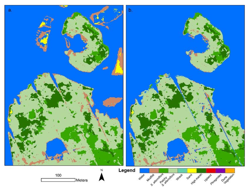
Remote Sens. 2019, 11, 1107                                                                        3 of 18

The decision to allow the Fire Island breach to evolve naturally facilitates monitoring to understand
the effect of this process on the surrounding salt marshes.
     Remote sensing monitoring can quantify essential attributes of the salt marsh landscape. Remote
sensing has been used to understand differences in salt marsh pond density and the total surface area
between ditched and unditched marshes [32]. Imagery and Light Detection and Ranging (LiDAR)
have been used to quantify pools and pannes and their landscape location [33]. Salt marsh change
analysis has been used to identify complex patterns of spatial and temporal variation [14], dramatic
conversions from high to low marsh [34], impacts of salt marsh restoration and Hurricane Sandy [35],
and identify the effect of SLR on salt marsh communities [36]. The combination of very high resolution
(VHR) satellite imagery and aerial imagery provided the necessary spatial and temporal resolution to
understand the dynamic coastal environment.
     This study mapped salt marsh habitat on Fire Island National Seashore (FIIS) utilizing object-based
image analysis (OBIA) with VHR satellite imagery. Multitemporal OBIA was utilized to analyze the
development and geospatial dynamics of pool and pannes with high spatial resolution aerial imagery
from 1994, 2011, 2013, 2015, and 2017. Change to pannes and pools and edge erosion were analyzed to
determine if they were significant components of salt marsh loss at FIIS. The use of remote sensing to
determine how protected areas are changing with high accuracy is vital to better manage these areas.
The objectives of this study are to (1) classify FIIS salt marsh with OBIA and VHR remote sensing
imagery data; (2) determine change rates for interior salt marsh pannes and pools and edge erosion
from 1994-2017; (3) determine the relationship between hydrological connectivity and panne expansion;
and (4) determine if edge erosion or panne/pool expansion increased surrounding the Hurricane Sandy
breach between 2011–2017.

2. Materials and Methods

2.1. Study Area
     Fire Island is a barrier island along the southern coast of Long Island, New York, of which 7924
hectares are managed and protected by the National Park Service (NPS) (Figure 1). Salt marsh is the
dominant land cover on the island comprising 26% of the protected area [37]. The bayside environment
is polyhaline [38]. The island’s geomorphology has been altered by urbanization, beach replenishment,
and inlet stabilization [39]. More frequent medium intensity storms have been linked with salt marsh
edge erosion [40]. Hurricane Sandy was a 1-in-500-year storm surge event that impacted the northeast
Atlantic coastal region on 24 Oct 2012 [41]. In 2003, Quickbird-2 satellite images were used to map
the study area with a focus on terrestrial and submerged aquatic vegetation [42]. Due to the limited
bayside tidal exchange, Fire Island’s salt marshes have a small tidal range of approximately 45.5 cm
between MLLW and MHHW [43]. SLR is outpacing accretion on the salt marshes of Fire Island as
determined by Surface Elevation Tables (SET) [5].
     Recent estimates of salt marsh change using aerial imagery from 1974 to 2005/2008 found a 14.1%
loss of salt marsh vegetation in a region including Fire Island [15]. The protected areas of FIIS include
the William Floyd Estate on the mainland and large bayside islands of Sexton, West Fire and East Fire
Island (Figure 1).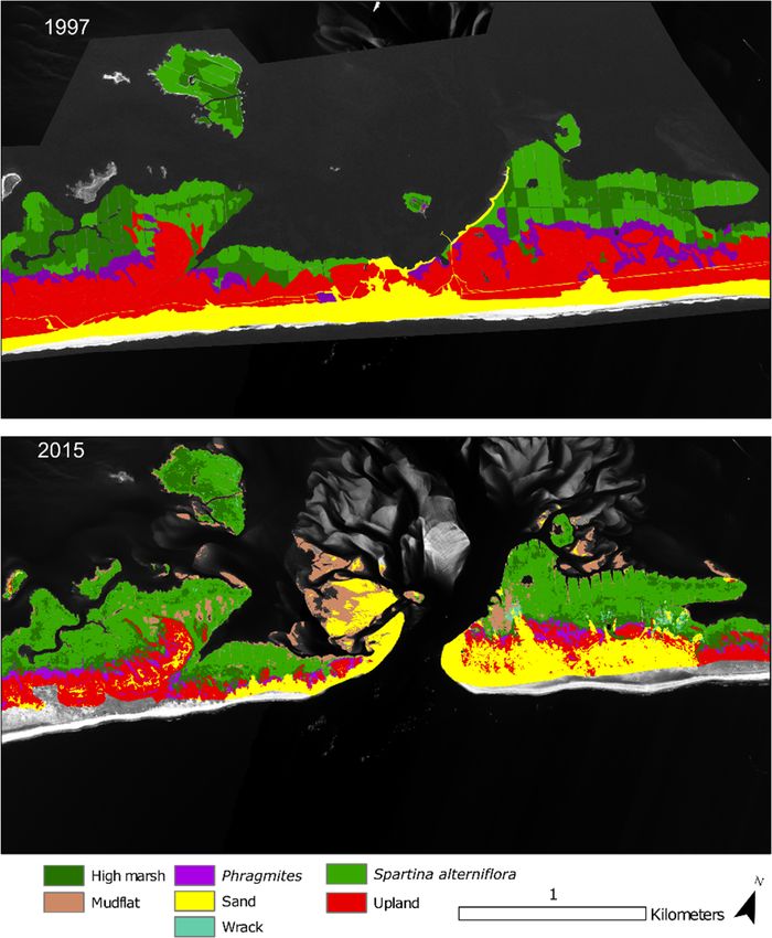
Remote Sens. 2019, 11,
       Sens. 2019, 11, 1107
                       x FOR PEER REVIEW                                                                          44 of 19
                                                                                                                     of 18

     Figure 1. (a) A mosaic of Worldview-2 and Worldview 3 imagery of Fire Island and Sentinel-2 satellite
     image
     Figureof1.the
                 (a).surrounding
                      A mosaic ofarea   (NIR, G, B displayed
                                      Worldview-2              as R, G,3 B).
                                                     and Worldview           (b) A post-Hurricane
                                                                          imagery                    Sandy
                                                                                    of Fire Island and      oblique
                                                                                                          Sentinel-2
     aerial view
     satellite     acquired
               image   of theby  U.S. Geological
                              surrounding   area Survey
                                                 (NIR, G,(USGS)  showing
                                                           B displayed      theG,bayside
                                                                        as R,     B). (b).salt marshes surrounding
                                                                                           A post-Hurricane  Sandy
     the breach
     oblique      [44].view
               aerial   (c) Aacquired
                              field photo
                                       by of theGeological
                                           U.S.  Fire Island Survey
                                                             National  Seashore
                                                                     (USGS)       (FIIS) salt
                                                                               showing    the marsh  landscape.
                                                                                               bayside salt marshes
     surrounding the breach [44]. (c). A field photo of the Fire Island National Seashore (FIIS) salt marsh
2.2. Data
     landscape.
     Satellite imageries were collected on 4/15/2015 and 5/25/2015 with Worldview-3 and Worldview-2
2.2. Data
sensors, respectively. Four-band National Agriculture Imagery Program (NAIP) data acquired between
2011 Satellite
      and 2017 and    the truewere
                 imageries      color National
                                      collected Aerial Photography
                                                 on 4/15/2015      andProgram
                                                                         5/25/2015(NAPP)
                                                                                       withdata  acquired in 1994
                                                                                             Worldview-3      and
were  used  to classify  the salt marshes  (Table 1). The aerial  imageries   were
Worldview-2 sensors, respectively. Four-band National Agriculture Imagery Program   collected  at a range of tidal
                                                                                                     (NAIP)  data
stages (Table
acquired       1). Change
           between           analysis
                      2011 and    2017was
                                       andalso
                                            the conducted  with a 1997
                                                true color National       classification
                                                                       Aerial            of FIIS
                                                                               Photography        performed
                                                                                               Program       with
                                                                                                         (NAPP)
true color aerial  photos  for the island and  verified with in situ field assessment   with  a highest
data acquired in 1994 were used to classify the salt marshes (Table 1). The aerial imageries were       achieved
overall accuracy
collected           of 87.5%
           at a range         [45,46].
                          of tidal  stages (Table 1). Change analysis was also conducted with a 1997
classification of FIIS performed with true color aerial photos for the island and verified with in situ
field assessment with a highest achieved overall accuracy of 87.5% [45,46].

     Table 1. The description of data used by acquisition date, spectral resolution (band wavelength when
     available), sensor or program, and spatial resolution. R = red, G = green, B = blue, NIR = near infrared,
     CB = coastal blue, Y = yellow, RE = Red edge.

                   Spectral Resolution (nm)                      Type                Spatial            Tidal Stage
    Date
                                                                                    Resolution           (NAVD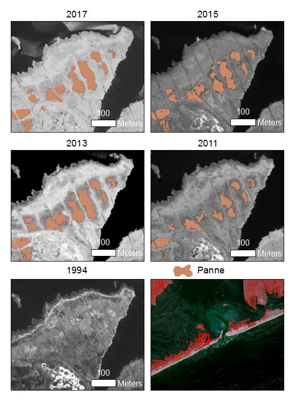
Remote Sens. 2019, 11, 1107                                                                                                5 of 18

      Table 1. The description of data used by acquisition date, spectral resolution (band wavelength when
      available), sensor or program, and spatial resolution. R = red, G = green, B = blue, NIR = near infrared,
      CB = coastal blue, Y = yellow, RE = Red edge.

                                                                                  Spatial Resolution        Tidal Stage
           Date               Spectral Resolution (nm)             Type
                                                                                          (m)             (NAVD 1988) *
       8 April 1994                     R, G, B                   NAPP                     1                      NA
                                                              LEICA ADS-52
       7 May 2011                    R, G, B, NIR                                          1                     0.02 m
                                                                 (NAIP)
     21 June 2013–22                                           ADS40-SH51
                                     R, G, B, NIR                                          1                     −0.21 m
        June 2013                                                (NAIP)
                              R (619–651), G (525–585), B     Leica ADS-100
       7 May 2015                                                                         0.5                    −0.29 m
                               (435–495), NIR (808–882)           (NAIP)
     9 August 2017 &          R (619–651), G (525–585), B     Leica ADS-100
                                                                                           1                     0.09 m
     27 August 2017            (435–495), NIR (808–882)           (NAIP)
                            CB (400–450), B (450–510), G
    25 May 2015 & 15          (510–580), Y (585–625), R
                                                              Worldview-2/3               0.5                    −0.29 m
       April 2015          (630–690), RE (705–745), NIR1
                             (770–895), NIR2 (860–1040)
                                                              Leica ALS 50-II
    8 January 2014–22                                                &                0.5 Digital
                                   Green and NIR                                                                  NA
        May 2014                                               Riegl sensor        Elevation Model
                                                                  9999609
                  * Average tidal stage across the acquisition as derived from USGS tidal gauge 01309225 [47].

2.3. Tidal Stage Effects
     The effects of the tidal stage at the time of imagery acquisition on mapped salt marsh extent has long
been recognized e.g., [48,49]. In this study, the tidal stage could impact the edge erosion calculations
and the panne analysis. Therefore, the highest tidal stage out of all the imageries was analyzed using
topobathymetric LiDAR, bathtub models, and the 2015 FIIS classification [50]. The method utilized the
topobathymetric LIDAR-derived Digital Elevation Model (DEM) to create a bathtub model, i.e., a binary
raster of inundated and non-inundated pixels, at the target tidal stage. The highest tidal stage of our
images was 35.66 cm MLLW or 14.3 cm above the North American Vertical Datum 1988 (NAVD 88)
occurring in 2017. The bathtub model was then used to determine areas mapped as vegetated in 2015
that were likely inundated at the 2017 image’s tidal stage. The method has been applied in Jamaica
Bay, New York, and was utilized in this study to understand the potential impact tidal stage had on the
aerial image classifications. These data provide an understanding of the uncertainty derived from
inundation that could occur in this analysis.

2.4. Object-Based Image Analysis
     OBIA begins with an unsupervised classification or segmentation dividing the image into
areas with similar spectral characteristics and spatial proximity [51]. This method used mean shift
segmentation: a hierarchical segmentation with demonstrated success in remote sensing and other
disciplines [52,53]. OBIA allows for the combination of spectral, spatial, and ancillary data and has
been shown to increase classification accuracy compared to pixel methodologies when using VHR
satellite imagery [54–56]. In this study, a multiscale segmentation approach was used, selecting
under segmented areas and resegmenting them at a finer segmentation scale [57,58] (Figure 2). This
study’s final segmentation was dual scale with 80% of objects segmented at a spectral radius of 13 and
minimum size of five pixels. The other 20% were segmented at a spectral radius of 8 and minimum
size of five pixels. Data processing and segmentation were conducted with Python 2.7 [59] and Orfeo
Toolbox 5.2 [60].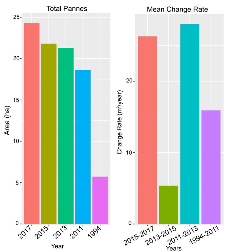
Remote Sens. 2019, 11, x FOR PEER REVIEW 6 of 19
study’s final segmentation was dual scale with 80% of objects segmented at a spectral radius of 13
and minimum size of five pixels. The other 20% were segmented at a spectral radius of 8 and
minimum
Remote Sens. size
2019,of
11,five
1107pixels. Data processing and segmentation were conducted with Python 2.76[59]
of 18
and Orfeo Toolbox 5.2 [60].
Figure 2. The data processing and classification workflow for classification of the Worldview-2 and
Figure 2. The data
Worldview-3 processing and classification workflow for classification of the Worldview-2 and
imagery.
Worldview-3 imagery.
The classification was composed of 10 categories including S. alterniflora, patchy S. alterniflora,
highThe classification
marsh, upland,was composed
dune of 10 categories
vegetation, including
sand, mudflat, S. alterniflora,
water, Phragmites, patchy
andS.wrack.
alterniflora,A
high marsh, upland, dune vegetation, 1-m
one-thousand-nine-hundred-and-thirteen 2 vegetation
sand, mudflat,plotwater,
data werePhragmites,
adapted to and wrack.
create A
training
one-thousand-nine-hundred-and-thirteen
data. The training data were composed of 1-m 2 vegetation
plots plot data were adapted
with a Braun–Blanquet to create
percent cover training
greater than
data.
≥50%. TheObjects
training data
that were composed
intersected trainingofpoints
plots with
were aselected,
Braun–Blanquet
resultingpercent cover
in a total greater
of 1964 than
training
≥50%. Objects
samples. that intersected
The species included training
in the highpoints
marsh were selected,
category wereresulting
S. patens,inD.a spicata,
total ofI. 1,964 training
frutescens, and
samples.
J. gerardii.The species
Percent included
cover in the high
differentiated the marsh category were
two S. alterniflora S. patens,
classes with theD.patchy
spicata,S.I. alterniflora
frutescens, class
and
J.being
gerardii.
betweenPercent cover
49 and differentiated
10% cover, and the theS.two S. alterniflora
alterniflora classes
class being withcover.
≥ 50% the patchy S. alterniflora
The vegetation plots
class
werebeing between 49within
predominantly and 10%thecover, and the
salt marsh S. alterniflora
environment class being
leading ≥ 50 sand
to water, % cover.
andThe vegetation
upland classes
plots
beingwere
trainedpredominantly
from samples within
gatheredthe salt marsh interpretation
by visual environment leading
and fieldtoknowledge.
water, sand The and Random
upland
classes being
Forest (RF) trainedwas
classifier from
usedsamples gathered
to classify the 2015 byWorldview-2/Worldview-3
visual interpretation andimage fielddata
knowledge. The
for vegetation
Random
mappingForestand the (RF) classifier
panne was classifications.
and edge used to classify the 2015 Worldview-2/Worldview-3 image data
for vegetation
Accuracymapping
assessment andwas
theconducted
panne andfor edge
theclassifications.
2015 Worldview-2/Worldview-3 image classification
usingAccuracy
a subset ofassessment was data.
the total training conducted
The datafor werethe 2015 split
randomly Worldview-2/Worldview-3
60% training and 40% for image testing.
classification
The training data usingwere
a subset
usedoftothe total
train thetraining
RF model.data.
AnThe data
error wereincluding
matrix randomlykappa,
split 60% trainingusers,
producers, and
40%
and for testing.
overall The training
accuracies data wereusing
was computed used tothetrain the data.
testing RF model. An error matrix including kappa,
producers,
The 2015users,
imageandclassification
overall accuracies was computed
was compared usingclassification
with a 1997 the testing data.
based on aerial imagery [45].
The 1997 classes of Reed grass marsh, high marsh, low marsh, and mosquito ditches were compared
with the 2015 classes of Phragmites, high marsh, and S. alterniflora classes accordingly. Mosquito
ditches in 1997 were included as vegetated area due to their small average width reported from 25.4 to
50.8 cm [61]. This width is below the minimum mapping unit of 0.25 ha for the 1997 classification [45]Remote Sens. 2019, 11, 1107 7 of 18
and the three-pixel width of the VHR classification. Change rate was calculated between 2015 and the
1997 salt marsh.
2.5. Change Analysis (1994–2017)
The panne and pool analysis, subsequently referred to as panne analysis, was conducted on
imageries from 1994 to 2017. The edge erosion change analysis was conducted for 1994 to 2011 and
2011 to 2017. Each image collection was segmented at a spectral radius of 10 and shape radius of 5 with
mean shift segmentation. This segmentation scale was adequate given the lower spectral resolution of
the aerial images. ArcMap 10.5 [62] was used to select segments which intersected the interior mud
or water areas of 2015 Worldview-2/Worldview-3 classifications, these segments comprised the 2015
pannes. The segments were then merged, creating a multitemporal segmentation. The classification
parameters included mean, median, standard deviation, simple indices (i.e., red band/blue band),
normalized difference vegetation index (NDVI) for those years with NIR, and the difference of each
band for the year of interest and subsequent year. The panne and edge classifications were trained with
objects that were either vegetated or non-vegetated. Their accuracies were verified with 522 randomly
selected points, which were assessed as vegetated or non-vegetated for each time period.
2.6. Statistical Analysis
Edge erosion was calculated for two periods from 1994 to 2011 and 2011 to 2017. The salt marsh
edge erosion was calculated based on starting edge length and the total area lost for each edge erosion
object. Welch ANOVAs were used to compare rates of change from 1994 to 2011 and 2011 to 2017
for both pannes and edge erosion. Least-squares means was used to compare the two edge erosion
rates and to see if edge erosion had increased following the hurricane breach and how this varied
between barrier island, bayside islands, and the mainland. A two-way ANOVA was used to compare
panne yearly change rates before and after the breach and between barrier island, bayside islands,
and the mainland. Annual salt marsh change rates were compared with a Kruskal–Wallis rank sum
test, a nonparametric statistical test, followed by a Wilcoxon rank sum test. Linear regression models
were used to test the relationship between edge erosion and distance from the breach for the period
2011 to 2017 for 2000 m in both directions. A beta regression ANOVA-like table was produced testing
the relationship between the percent change from 2015 to 2017 of interior areas with and without
mosquito ditch hydrological connections. All statistical analysis was done within the R 3.5.1 statistical
environment [63].
3. Results
3.1. OBIA Classification
The 2015 Worldview-2/Worldview-3 image classification achieved an overall accuracy of 92.75%
(Table 2). Visual inspections revealed an appealing result with an appropriate gradient from S. alterniflora,
high marsh, Phragmites, and upland vegetation (Figure 3). Errors were mostly between the two types
of S. alterniflora due to their spectral similarities and early seasonal acquisition date of the imagery.
There was no confusion between mudflat/water and other classes making this classification an ideal
baseline for change analysis.
The 2015 Worldview-2/Worldview-3 imagery classification was compared with a 1997 classification
conducted with aerial imagery. When comparing salt marsh vegetation between the two periods a
reduction from 531.27 ha to 505.95 ha was observed or 1.41 ha y−1 .Reference data
Hig Patchy
Dune S. User’s
h Mudfl Phragmit S. Upla Wat Wrac
Class Vegetati Sand alternifl Accura
mars at es alternifl nd er k
on
Remote Sens. 2019, 11, 1107 h
ora 8 of 18
cy
ora
Dune Veg. 36 0 0 0 0 0 0 0 0 0 100
High marsh
Table 2. An error0 matrix61for the 2015
0 Worldview-2/Worldview-3
1 0 0
classification 6 Island National
of Fire 2 0
Seashore. 0 87.1
Classified data
Mudflat 0 0 30 0 0 0 0 0 0 0 100
Reference Data
Phragmites 0 0 0 15 0 0 0 0 0 0 100
Dune High Patchy S. S. User’s
Sand Class
0 0 Marsh0 Mudflat Phragmites
Vegetation 0 Sand
26 alterniflora0 alterniflora 0Upland Water
0 Wrack 0Accuracy 0 100
Patchy S. Dune Veg. 36 0 0 0 0 0 0 0 0 0 100
0
High marsh 0 0 61 0 0 01 00 0 34 6 14 2 00 0 0 87.1 0 70.8
alterniflora
Mudflat 0 0 30 0 0 0 0 0 0 0 100
S. alterniflora Phragmites0 0
3 0
0 0
0 15 0
0 0
0 0
79 0 0
0 0
0 100 0 96.3
Classified data
Upland Sand0 0 0 0 0 0 00 26 0 0 0 0 0 0 040 0 0 100 0 100
Water Patchy0S.
0
0 0
0 0
00 0
0 34
0 14
0 0 0
0 0
40 70.8 0 100
alterniflora
Wrack 0 1 0 0 1 0 0 0 0 10 83.3
S. alterniflora 0 3 0 0 0 0 79 0 0 0 96.3
Producer’s Upland 0 0
OA:
100 93.8 100 0 93.80 0
96.3 0
100 0
79.840 0
95.2 0
100 100 100
Accuracy Water 0 0 0 0 0 0 0 0 40 0 100 92.75
Wrack 0 1 0 0 1 0 0 0 0 10 83.3
Table 2: An
Producer’s error
100 matrix for the 100
93.8 2015 Worldview-2/Worldview-3
93.8 96.3 100 classification
79.8 of Fire 100
95.2 Island100
National
OA:
Accuracy 92.75
Seashore.
Figure 3. (a) The 2015 Worldview-2/Worldview-3 image classification of salt marshes in FIISs. (b) A
section of FIIS directly to the west of the old inlet breach. (c) The Floyd Bennet estate, a section of FIIS
on the mainland.
3.2. Tidal Stage Effect
The 2017 NAIP imageries were acquired at an approximate tidal stage of 35.66 cm above
MLLW at U.S. Geological Survey (USGS) 01305575 at Watch Hill [43]. The 2014 DEM derived from
topobathymetric LiDAR was used to determine how much inundation of S. alternilflora would be
expected at this elevation. The analysis found 7.39% of the 2015 classification’s S. alterniflora classes
were inundated. The indundation could be subcanopy and have little impact on the 2017 classification.FIIS on the mainland.
3.2. Tidal Stage Effect
The 2017 NAIP imageries were acquired at an approximate tidal stage of 35.66 cm above MLLW
at U.S. Geological Survey (USGS) 01305575 at Watch Hill [43]. The 2014 DEM derived from
Remote Sens. 2019, 11, 1107 9 of 18
topobathymetric LiDAR was used to determine how much inundation of S. alternilflora would be
expected at this elevation. The analysis found 7.39% of the 2015 classification’s S. alterniflora classes
were
The inundated.
areas of modeled The inundation
indundationwere
could beprevalent
most subcanopy and have ditches,
in mosquito little impact on the
sandbars, and2017
interior
classification. The
mudflats (Figure 4). areas of modeled inundation were most prevalent in mosquito ditches, sandbars,
and interior mudflats (Figure 4).
Figure 4. (a)
Figure 4. (a).The
The2015
2015 Worldview-2
Worldview-2 and
and Worldview-3 Classificationfor
Worldview-3 Classification foraasection
sectionofofFire
FireIsland
Islandeast
east of
the breach. (b) The modeled tidal inundation of the 2015 classification at a tidal stage of 14.3
of the breach. (b). The modeled tidal inundation of the 2015 classification at a tidal stage of 14.3 cm cm above
NAVD 88, which
above NAVD corresponded
88, which to the to
corresponded highest tidal stage
the highest of theofimagery
tidal stage usedused
the imagery in the study.
in the study.
3.3. Change Analysis (1994–2017)
3.3. Change Analysis (1994-2017)
The panne change analysis achieved overall accuracy > 85% for all years (Table 3). However
The panne change analysis achieved overall accuracy > 85% for all years (Table 3). However
since these classifications were being used in tandem it is important to note that propogated percent
since these classifications were being used in tandem it is important to note that propogated percent
error calculated by the square root of the sum of squares was 16.7, 10.2, 11.8, and 13.1 for 1994–2011,
error calculated by the square root of the sum of squares was 16.7, 10.2, 11.8, and 13.1 for 1994–2011,
2011–2013,
2011–2013,2013–2015,
2013–2015,and 2015–2017,
and 2015–2017,respectively.
respectively.Models withwith
Models low overall accuracies
low overall were evaluated
accuracies were
and manually digitized when necessary. The analysis included 475 pannes mapped
evaluated and manually digitized when necessary. The analysis included 475 pannes mapped in 2015 thatinwere
>2015
10 square
that weremeters. In 2015,
> 10 square the mean
meters. panne
In 2015, size was
the mean panne441.6
sizemwas
compared to the 1994tomean
441.6 m compared size of
the 1994
121.4
meanm. Inof1994,
size 121.4257
m. of
In the 475
1994, 257pannes were
of the 475 vegetated.
pannes The meanThe
were vegetated. yearly
meanrates of panne
yearly rates ofchange
panne for
each of the −1 for 2015–2017,
m2 y15.91
change for periods were
each of the 25.00,were
periods 5.34, 25.00,
27.98,5.34,
and 27.98,
15.91 and 2013–2015,
m2 y-1 for 2015–2017, 2011–2013,
2013–2015,
and 1994–2011, respectively (Figure 5). There were statistical differences between the yearly change
rates (H (3 ) = 30.097, p < 0.001) were compared with the Wilcoxon rank sum test (Table 4). There were
significant differences between edge erosion rates between 1994 and 2011 and 2011 and 2017 (F1, 1597
= 206.06, pRemote Sens. 2019, 11, 1107 10 of 18
Edge erosion to the west of the breach from 2011–2017 had no trend (F1,94 = 1.5, p = 0.22) and an R2
of 0.02.
Table 3. Panne and edge overall classification accuracies, 1994–2015.
Year Overall Accuracy (%) Image Source Spatial Resolution (m)
2017 92.4 NAIP 1
2015 89.3 NAIP 0.5
2013 95.0 NAIP 1
2011 91.1 NAIP 1
Remote Sens. 2019, 1994
11, x FOR PEER REVIEW
85.88 NAPP 1 11 of 19
Figure 5.5. Interior
Figure Interiorpannes
pannestotal area
total andand
area change ratesrates
change fromfrom
(1994–2017) both the
(1994–2017) average
both yearly change
the average yearly
rates of a time period and total area of pannes and pools.
change rates of a time period and total area of pannes and pools.Remote Sens. 2019, 11, 1107 11 of 18
Table 4. Wilcoxon rank sum test between annual panne change rates.
Years 2017–2015 2015–2013 2013–2011
2015–2013 p < 0.05
2013–2011 p = 0.72 p < 0.72
2011–1994 p < 0.001 p < 0.72 p < 0.001
Remote Sens. 2019, 11, x FOR PEER REVIEW 12 of 19
Figure 6. Edge
Figure erosion
6. Edge rates
erosion compared
rates comparedby bytime
timeperiod (1994–2011,2011–2017)
period (1994–2011, 2011–2017)andand location
location (barrier
(barrier
island, mainland,
island, or back
mainland, bay
or back island)
bay island)with
withleast
least square meanswith
square means withBonferroni
Bonferroni p-value
p-value adjustment.
adjustment.
Location/dates thatthat
Location/dates share letters
share did
letters not
did notdemonstrate
demonstrate significant differences
significant differences (p(p > 0.05).
> 0.05).
Table 4. Wilcoxon rank sum test between annual panne change rates.
Years 2017–2015 2015–2013 2013–2011
2015-2013 p < 0.05
2013-2011 p = 0.72 p < 0.72
2011-1994 p < 0.001 p < 0.72 p < 0.001Remote Sens. 2019, 11, 1107 12 of 18
Remote Sens. 2019, 11, x FOR PEER REVIEW 13 of 19
Figure 7. Panne classification from 1994 to 2017 for an area to the west of the old inlet breach. Each inset
Figure 7. Panne classification from 1994 to 2017 for an area to the west of the old inlet breach. Each
has the corresponding years NIR in panchromatic or red band in 1994. The locus map is a Sentinel-2
inset has the corresponding years NIR in panchromatic or red band in 1994. The locus map is a
image from 5/21/2016.
Sentinel-2 image from 5/21/2016.
4. Discussion
4. Discussion
The change analysis between the 1997 classification and the 2015 classification revealed salt marsh
The change
loss (Figure analysis
8). High marshbetween
area fellthe
from 1997
199.6classification andPrevious
ha to 109.8 ha. the 2015studies classification
mapping revealed
salt marshsalt
marsh loss
change from (Figure
1974 to8).2005/2008
High marsh areaentirety
for the fell fromof 199.6
Long ha to 109.8
Island, NY ha. foundPrevious
similarstudies
change, mapping
including salt
a
marsh change from 1974 to 2005/2008 for the entirety of Long Island, NY
35.5% reduction in the high marsh for a region from Fire Island inlet to Smith Point, and a decrease in found similar change,
including a on
Phragmites 35.5%
the reduction
south shore in[15].
the high marsh for aof
The conversion region
upland from
andFire Island inlet
Phragmites to Smith
to low Point,
and high and
marsh
a decrease in Phragmites on the south shore [15]. The conversion of upland
categories suggests salt marsh migration in response to SLR. The utility of the comparison between and Phragmites to low
and high marsh categories suggests salt marsh migration
1997 and 2015 was limited due to the different classification schemes. in response to SLR. The utility of the
comparison between
In general, 1997 anddemonstrated
pannes/pools 2015 was limited due periods
several to the different classification
of statistically schemes.
significant expansion. Of
the 475 pannes, 46% were present in 1994. Meaning there was a doubling of pools andexpansion.
In general, pannes/pools demonstrated several periods of statistically significant pannes from Of
the 475 pannes, 46% were present in 1994. Meaning there was a doubling of
1994 to 2015. Two hundred and twelve of the 475 pannes were in areas classified as high marsh in 1997. pools and pannes from
1994 topannes
These 2015. Two hundred
accounted and twelve
for 12.51 ha out of of the 475ofpannes
a total 21.81 ha,were
i.e.,inthe
areas classified
largest area ofas high marsh
pannes occurred in
1997. These pannes accounted for 12.51 ha out of a total of 21.81 ha, i.e.,
in the high marsh. These non-vegetated pannes/pools are essentially tidal mudflats which provide the largest area of pannes
occurred
some in theecosystems
essential high marsh.services.
These non-vegetated
However, ecosystem pannes/pools
serviceare essentially
valuations tidal salt
suggest mudflats
marshwhich
to be
provide some essential ecosystems services.
over five times more valuable than mudflats [64]. However, ecosystem service valuations suggest salt
marsh to be over five times more valuable than mudflats [64].
The expected evolution of an interior salt marsh pool is expansion until hydrological connectivity
The expected
is established leadingevolution
to drainage ofand
an possible
interiorvegetation
salt marsh pool is
regrowth [22].expansion until pannes/pools
In our analysis, hydrological
connectivity is established leading to drainage and possible vegetation
connected to mosquito ditches in 2015 had a mean change rate of −3.52 m y compared to 30.87 2 −1 regrowth [22]. mIn2 our
y−1
analysis, pannes/pools connected to mosquito ditches in 2015 had a mean change rate of −3.52 m2 y-1
compared to 30.87 m2 y-1 for non-hydrologically connected pannes/pools. This is encouraging for theRemote Sens. 2019, 11, 1107 13 of 18
Remote Sens. 2019, 11, x FOR PEER REVIEW 14 of 19
for non-hydrologically connected pannes/pools. This is encouraging for the possibility of vegetation
possibility However,
regrowth. of vegetation regrowth.
natural However,
creeks are natural
infrequent creeksfeatures
landscape are infrequent landscaperelatively
having remained features
havingfrom
stable remained
1930 to relatively
2007 [61]. stable from 1930
In contrast to 2007ditches
mosquito [61]. Inare
contrast
common mosquito
acrossditches are common
Fire Island, leading
across
to Fire Island,
hydrological leading to
connectivity hydrological
with connectivity
mosquito ditches with mosquito
being common. However, ditches being
besides common.
providing a
However, besides
hydrological providing
connection, a hydrological
mosquito connection,
ditches likely mosquitoby
drive drowning ditches likely
altering marshdrive drowningand
hydrology, by
altering marsh
plugged mosquito hydrology, and plugged
ditches cause mosquito
subsidence and lossditches cause
of salt marsh subsidence and loss
function [65]. of salt marsh
Additionally, the
function
berms [65]. Additionally,
surrounding ditches can thelead
berms surrounding
to poor drainage ditches can lead
[66]. Highly to poor
variable drainage [66].
accumulation Highly
of sediment
variable
in accumulation
Fire Island’s mosquito ofditches
sediment hasin
ledFire Island’s
to the mosquito
infill of ditches
some ditches andhas ledtotonothe
little infill of some
accumulation in
ditches[61]
others and(Figure
little to8).noThe
accumulation
varied rate in others [61]
of infilling could(Figure 8). The varied
be influencing rate of
observed infilling
rates could be
of panne/pool
influencing observed
expansion. The landscape rates of panne/pool
legacy expansion.ditches
of the mosquito The landscape legacy offactor
is a site-specific the mosquito ditchesfor
that is critical is
a site-specific factor that is critical for
understanding salt marsh change on Fire Island. understanding salt marsh change on Fire Island.
Figure
Figure 8. Land cover
8. Land cover of
of the
the area
area surrounding
surrounding thethe 2012
2012 Fire
Fire Island
Island breach
breach for
for 1997
1997 and
and 2015.
2015. Land
Land
cover change both due to the breach and overwash are evident in the 2015 classification.
cover change both due to the breach and overwash are evident in the 2015 classification. Spartina Spartina
alterniflora
alterniflora classes
classes are
are shown
shown asas aa single
single class
class due
due to
to the
the 1997 class no
1997 class no differentiating
differentiating between
between percent
percent
cover. Upland and dune vegetation classes are also shown as a single
cover. Upland and dune vegetation classes are also shown as a single class. class.
Whether vegetation regrowth occurred within the pannes/pools is a critical question. Vegetation
Whether vegetation regrowth occurred within the pannes/pools is a critical question.
regrowth is limited by the growth range of S. alterniflora at the site. The lowest elevation of living
Vegetation regrowth is limited by the growth range of S. alterniflora at the site. The lowest elevation
S. alterniflora at the site was 25.7 cm below NAVD 1988 [67]. The minimum growing elevation of
of living S. alterniflora at the site was 25.7 cm below NAVD 1988 [67]. The minimum growing
S. alterniflora
elevation foralterniflora
of S. FIIS was determined
for FIIS wasusing the tidalusing
determined rangethe
of 45.5
tidalcm and the
range methods
of 45.5 of [10].
cm and Finding
the methods
aofminimum growth
[10]. Finding a elevation
minimumofgrowth
12.7 cm elevation
below NAVD 1988,cm
of 12.7 which is a more
below NAVD conservative
1988, whichestimate than
is a more
the observed minimum growth elevation. Six of the 475 pannes analyzed were below
conservative estimate than the observed minimum growth elevation. Six of the 475 pannes analyzed the vegetation
range of S. alterniflora
were below at the site,
the vegetation rangemeaning vegetation at
of S. alterniflora could
the grow on nearlyvegetation
site, meaning all of the observed pannes.
could grow on
nearly all of the observed pannes. However, only 30 of the 475 2015 pannes/pools were entirely
vegetated in 2017. Complete vegetation regrowth was rare but did occur in the pannes and pools
analyzed.Remote Sens. 2019, 11, 1107 14 of 18
However, only 30 of the 475 2015 pannes/pools were entirely vegetated in 2017. Complete vegetation
regrowth was rare but did occur in the pannes and pools analyzed.
Significant increases in edge erosion were observed following the breach. These areas likely
experienced changes in currents, wave energy, or LMSL. For example, the William Floyd estate site
saw no significant difference in edge erosion before and after the breach. This site is approximately
8 km away from the breach and approximately 5 km from the stabilized Moriches Inlet. In contrast,
the area immediately surrounding the breach to the east experienced significant loss from increased
edge erosion. An increase in edge erosion as you neared the breach was evident towards the east.
However, there was no such trend to the west of the breach. The high variability of the bayside salt
marsh erosion demonstrates the importance of geospatial monitoring to understand how these systems
are changing spatially. As previous studies reported, Surface Elevation Table (SET)-derived accretion
estimates at the site are below the rates of SLR [5]. FIIS’ wilderness areas have little infrastructure
limiting the migration of salt marsh. However, the islands width and interconnectedness of the barrier
island systems means salt marsh migration alone will not maintain the barrier island.
The bayside of barrier islands have low energy and small tidal range (Watch Hill, NY on Fire
Island’s tidal range is 45.5 cm between MLLW and MHHW [43]), which can result in slower expansion
of pools due to edge erosion [25]. The establishment of an inlet can cause an increase in tidal
range; however, there were no statistical differences between panne/pool expansion rates between the
examined time periods (1994–2011 and 2011–2017). Possibly due to the scarcity of pools in our analysis
which would be expected to expand more rapidly with increased tidal range. The breach caused by
Hurricane Sandy did not appear to accelerate or slow the interior salt marsh change. However, edge
erosion significantly increased following the breach. Continued monitoring is necessary to determine
if the observed trend continues.
5. Conclusions
This study evaluated panne/pool development and fluctuations with remote sensing, identifying
spatial and temporal patterns of coastal marsh habitat change in a protected National Seashore. Remote
sensing methods were essential for understanding how these protected salt marshes changed from
1994 to 2017. This analysis was contingent on the proliferation of remote sensing data which allowed
for the synthesis of multiple data types to better understand salt marsh trends and dynamics. Change
analysis demonstrated that panne/pool expansion and edge erosion accounted for the majority of
salt marsh loss. The losses were partly driven by an increase in edge erosion observed following the
breach. Vegetation regrowth occurred with pannes/pools demonstrating increased regrowth when
hydrologically connected to a mosquito ditch or channel. The pannes/pools analyzed were not in
equilibrium in the two decades analyzed instead demonstrating a long-term trend of expansion.
There is a need for increased salt marsh monitoring for determining where, when, and how salt
marshes are changing. This study presents a methodology for salt marsh classification and change
analysis of pannes and edge erosion. The aerial imagery classifications achieved satisfactory overall
accuracies (> 85%) as suggested by Thomlison et al. [68], however, propagated error when conducting
the change analyses was a concern. NAIP imagery is an ideal data source in regards to spatial, temporal
and spectral resolution with several caveats. The lack of a NIR band led to a decrease in accuracy
due to vegetated and non-vegetated pannes appearing spectrally similar. Additionally, aerial image
acquisitions had variable quality and tidal stages at time of acquisition which limited the accuracy
of particular years. Finally, the data are only available for the USA. The workflow used in this study
allowed for rapid classification and change analysis of salt marsh environments. The biennial collection
of NAIP imagery makes it uniquely suited for the low-cost continuation of high-resolution salt marsh
monitoring into the future.
Author Contributions: Conceptualization, A.C. and Y.W.; Formal Analysis, Y.W.; Funding Acquisition, Y.W.;
Investigation, A.C. and Y.W.; Methodology, A.C. and Y.W.; Project administration, Y.W.; Resources, Y.W.; Software,Remote Sens. 2019, 11, 1107 15 of 18
Y.W.; Supervision, Y.W.; Validation, A.C.; Visualization, A.C.; Writing—Original Draft, A.C.; Writing—Review &
Editing, A.C. and Y.W.
Funding: This research was funded by U.S. National Park Service, grant number: P14AC00230.
Acknowledgments: This project was funded by the Northeast Coastal and Barrier Network (NCBN) of the
National Park Service (NPS)’s Inventory & Monitoring Program under the Task Agreement Number P14AC00230.
We appreciate the guidance and support of Sara Stevens, Dennis Skidds, Bill Thompson, and Charles Roman of
the NPS NCBN and North Atlantic Coast CESU. The authors appreciate the assistance by administrators and
professionals from Fire Island National Seashore (FIIS), particularly Jordan Raphael for his expertise, insights,
field guidance, and logistic support. Additionally, the authors would like to thank the three anonymous reviewers
for their comments and constructive criticism.
Conflicts of Interest: The authors declare no conflict of interest.
References
1. Zedler, J.B.; Kercher, S. Wetland Resources: Status, Trends, Ecosystem Services, and Restorability. Annu. Rev.
Environ. Resour. 2005, 30, 39–74. [CrossRef]
2. Barbier, E.B.; Hacker, S.D.; Kennedy, C.; Koch, E.W.; Stier, A.C.; Silliman, B.R. The Value of Estuarine and
Coastal Ecosystem Services. Ecol. Monogr. 2011, 81, 169–193. [CrossRef]
3. Gedan, K.B.; Silliman, B.R.; Bertness, M.D. Centuries of Human-Driven Change in Salt Marsh Ecosystems.
Annu. Rev. Mar. Sci. 2009, 1, 117–141. [CrossRef] [PubMed]
4. Crain, C.M.; Gedan, K.B.; Dionne, M. Tidal Restrictions and Mosquito Ditching in New England Marshes. In
Human Impacts on Salt Marshes: A Global Perspective; University of California Press: Berkeley, CA, USA, 2009;
pp. 149–169.
5. Crosby, S.C.; Sax, D.F.; Palmer, M.E.; Booth, H.S.; Deegan, L.A.; Bertness, M.D.; Leslie, H.M. Salt Marsh
Persistence is Threatened by Predicted Sea-Level Rise. Estuar. Coast. Shelf Sci. 2016, 181, 93–99. [CrossRef]
6. Watson, E.B.; Raposa, K.B.; Carey, J.C.; Wigand, C.; Warren, R.S. Anthropocene Survival of Southern New
England’s Salt Marshes. Estuaries Coasts 2017, 40, 617–625. [CrossRef] [PubMed]
7. Wigand, C.; Roman, C.T.; Davey, E.; Stolt, M.; Johnson, R.; Hanson, A.; Watson, E.B.; Moran, S.B.; Cahoon, D.R.;
Lynch, J.C. Below the Disappearing Marshes of an Urban Estuary: Historic Nitrogen Trends and Soil Structure.
Ecol. Appl. 2014, 24, 633–649. [CrossRef] [PubMed]
8. Altieri, A.H.; Bertness, M.D.; Coverdale, T.C.; Herrmann, N.C.; Angelini, C. A Trophic Cascade Triggers
Collapse of a Salt-marsh Ecosystem with Intensive Recreational Fishing. Ecology 2012, 93, 1402–1410.
[CrossRef]
9. Deegan, L.A.; Johnson, D.S.; Warren, R.S.; Peterson, B.J.; Fleeger, J.W.; Fagherazzi, S.; Wollheim, W.M. Coastal
Eutrophication as a Driver of Salt Marsh Loss. Nature 2012, 490, 388–392. [CrossRef]
10. Kirwan, M.L.; Guntenspergen, G.R. Influence of Tidal Range on the Stability of Coastal Marshland. J. Geophys.
Res. Earth Surf. 2010, 115. [CrossRef]
11. Kirwan, M.L.; Murray, A.B.; Boyd, W.S. Temporary Vegetation Disturbance as an Explanation for Permanent
Loss of Tidal Wetlands. Geophys. Res. Lett. 2008, 35. [CrossRef]
12. Holdredge, C.; Bertness, M.D.; Altieri, A.H. Role of Crab Herbivory in Die-Off of New England Salt Marshes.
Conserv. Biol. 2009, 23, 672–679. [CrossRef]
13. Kearney, M.S.; Rogers, A.S.; Townshend, J.R.; Rizzo, E.; Stutzer, D.; Stevenson, J.C.; Sundborg, K. Landsat
Imagery shows Decline of Coastal Marshes in Chesapeake and Delaware Bays. EOS Trans. Am. Geophys. Union
2002, 83, 173–178. [CrossRef]
14. Schepers, L.; Kirwan, M.; Guntenspergen, G.; Temmerman, S. Spatio-temporal Development of Vegetation
Die-off in a Submerging Coastal Marsh. Limnol. Oceanogr. 2017, 62, 137–150. [CrossRef]
15. Cameron Engineering and Associates. Long Island Tidal Wetlands Trends Analysis; New England Interstate
Water Pollution Control Commission: Lowell, MA, USA, 2015; 207p.
16. Watson, E.B.; Wigand, C.; Davey, E.W.; Andrews, H.M.; Bishop, J.; Raposa, K.B. Wetland Loss Patterns
and Inundation-Productivity Relationships Prognosticate Widespread Salt Marsh Loss for Southern New
England. Estuaries Coasts 2017, 40, 662–681. [CrossRef]
17. Schieder, N.W.; Walters, D.C.; Kirwan, M.L. Massive Upland to Wetland Conversion Compensated for
Historical Marsh Loss in Chesapeake Bay, USA. Estuaries Coasts 2018, 41, 940–951. [CrossRef]Remote Sens. 2019, 11, 1107 16 of 18
18. Schuerch, M.; Spencer, T.; Temmerman, S.; Kirwan, M.L.; Wolff, C.; Lincke, D.; McOwen, C.J.; Pickering, M.D.;
Reef, R.; Vafeidis, A.T. Future Response of Global Coastal Wetlands to Sea-Level Rise. Nature 2018, 561, 231.
[CrossRef]
19. Marsh, A.; Blum, L.K.; Christian, R.R.; Ramsey, E.; Rangoonwala, A. Response and Resilience of Spartina
Alterniflora. J. Coast. Conserv. 2016, 20, 335–350. [CrossRef]
20. Alber, M.; Swenson, E.M.; Adamowicz, S.C.; Mendelssohn, I.A. Salt Marsh Dieback: An Overview of Recent
Events in the US. Estuar. Coast. Shelf Sci. 2008, 80, 1–11. [CrossRef]
21. Kearney, M.S.; Turner, R.E. Microtidal Marshes: Can these Widespread and Fragile Marshes Survive
Increasing Climate–sea Level Variability and Human Action? J. Coast. Res. 2016, 32, 686–699. [CrossRef]
22. Wilson, K.R.; Kelley, J.T.; Croitoru, A.; Dionne, M.; Belknap, D.F.; Steneck, R. Stratigraphic and Ecophysical
Characterizations of Salt Pools: Dynamic Landforms of the Webhannet Salt Marsh, Wells, ME, USA.
Estuaries Coasts 2009, 32, 855–870. [CrossRef]
23. Cowardin, L.M.; Carter, V.; Golet, F.C.; LaRoe, E.T. Classification of Wetlands and Deepwater Habitats of the
United States; U.S. Department of the Interior: Washington, DC, USA, 1979; 131p.
24. Wilson, C.A.; Hughes, Z.J.; FitzGerald, D.M.; Hopkinson, C.S.; Valentine, V.; Kolker, A.S. Saltmarsh Pool and
Tidal Creek Morphodynamics: Dynamic Equilibrium of Northern Latitude Saltmarshes? Geomorphology
2014, 213, 99–115. [CrossRef]
25. Mariotti, G. Revisiting Salt Marsh Resilience to Sea Level Rise: Are Ponds Responsible for Permanent Land
Loss? J. Geophys. Res. Earth Surf. 2016, 121, 1391–1407. [CrossRef]
26. Hapke, C.J.; Brenner, O.; Hehre, R.; Reynolds, B.J. Coastal Change from Hurricane Sandy and the 2012–13
Winter Storm Season—Fire Island; Geological Survey Open-File Report; U.S. Geological Survey: Reston, VA,
USA, 2013.
27. Leatherman, S.P. Geomorphic and Stratigraphic Analysis of Fire Island, New York. Mar. Geol. 1985, 63,
173–195. [CrossRef]
28. Friedrichs, C.T.; Perry, J.E. Tidal Salt Marsh Morphodynamics: A Synthesis. J. Coast. Res. 2001, 7–37.
Available online: https://www.jstor.org/stable/25736162 (accessed on 15 January 2019).
29. Courtemanche, R.P., Jr.; Hester, M.W.; Mendelssohn, I.A. Recovery of a Louisiana Barrier Island Marsh Plant
Community Following Extensive Hurricane-Induced Overwash. J. Coast. Res. 1999, 15, 872–883.
30. Roman, C.T.; King, D.R.; Cahoon, D.R.; Lynch, J.C.; Appleby, P.G. Evaluation of Marsh Development Processes at
Fire Island National Seashore: Recent and Historic Perspectives; National Park Service: Boston, MA, USA, 2007.
31. Silvestri, S.; D’Alpaos, A.; Nordio, G.; Carniello, L. Anthropogenic Modifications can significantly Influence
the Local Mean Sea Level and Affect the Survival of Salt Marshes in Shallow Tidal Systems. J. Geophys. Res.
Earth Surf. 2018, 123, 996–1012.
32. Adamowicz, S.C.; Roman, C.T. New England Salt Marsh Pools: A Quantitative Analysis of Geomorphic and
Geographic Features. Wetlands 2005, 25, 279–288. [CrossRef]
33. Millette, T.L.; Argow, B.A.; Marcano, E.; Hayward, C.; Hopkinson, C.S.; Valentine, V. Salt Marsh
Geomorphological Analyses Via Integration of Multitemporal Multispectral Remote Sensing with LIDAR
and GIS. J. Coast. Res. 2010, 26, 809–816. [CrossRef]
34. Smith, S.M. Vegetation Change in Salt Marshes of Cape Cod National Seashore (Massachusetts, USA)
between 1984 and 2013. Wetlands 2015, 35, 127–136. [CrossRef]
35. Campbell, A.; Wang, Y.; Christiano, M.; Stevens, S. Salt Marsh Monitoring in Jamaica Bay, New York from
2003 to 2013: A Decade of Change from Restoration to Hurricane Sandy. Remote Sens. 2017, 9, 131. [CrossRef]
36. Sun, C.; Fagherazzi, S.; Liu, Y. Classification Mapping of Salt Marsh Vegetation by Flexible Monthly NDVI
Time-Series using Landsat Imagery. Estuar. Coast. Shelf Sci. 2018, 213, 61–80. [CrossRef]
37. McElroy, A.; Benotti, M.; Edinger, G.; Feldmann, A.; O’Connell, C.; Steward, G.; Swanson, R.L.;
Waldman, J. Assessment of Natural Resource Conditions: Fire Island National Seashore; Natural Resource
Report NPS/NRPC/NRR; National Park Service: Fort Collins, CO, USA, 2009.
38. Hair, M.E.; Buckner, S. An Assessment of the Water Quality Characteristics of Great South Bay and Contiguous
Streams; Adelphi University Institute of Marine Science: Garden City, NY, USA, 1973.
39. Lentz, E.E.; Hapke, C.J. Geologic Framework Influences on the Geomorphology of an Anthropogenically
Modified Barrier Island: Assessment of Dune/Beach Changes at Fire Island, New York. Geomorphology 2011,
126, 82–96. [CrossRef]Remote Sens. 2019, 11, 1107 17 of 18
40. Leonardi, N.; Ganju, N.K.; Fagherazzi, S. A Linear Relationship between Wave Power and Erosion Determines
Salt-Marsh Resilience to Violent Storms and Hurricanes. Proc. Natl. Acad. Sci. USA 2016, 113, 64–68.
[CrossRef]
41. Aerts, J.C.; Lin, N.; Botzen, W.; Emanuel, K.; de Moel, H. Low-Probability Flood Risk Modeling for New York
City. Risk Anal. 2013, 33, 772–788. [CrossRef]
42. Wang, Y.; Traber, M.; Milstead, B.; Stevens, S. Terrestrial and Submerged Aquatic Vegetation Mapping in Fire
Island National Seashore using High Spatial Resolution Remote Sensing Data. Mar. Geod. 2007, 30, 77–95.
[CrossRef]
43. U.S. Geological Survey (USGS). USGS Surface-Water Daily Data for New York. Watch Hill, NY, USA, 2017.
Available online: https://waterdata.usgs.gov/ny/nwis/uv?site_no=01305575 (accessed on 15 January 2019).
44. Morgan, K.L.M.; Krohn, M.D. Post-Hurricane Sandy Coastal Oblique Aerial Photographs Collected from Cape
Lookout, North Carolina, to Montauk, New York, November 4–6, 2012; U.S. Geological Survey Data Series 858;
U.S. Geological Survey: Reston, VA, USA, 2014. [CrossRef]
45. Conservation Management Institute, NatureServe, and New York Natural Heritage Program. Fire Island
National Seashore Vegetation Inventory Project—Spatial Vegetation Data; National Park Service: Denver, CO, USA,
2002. Available online: https://www.sciencebase.gov/catalog/item/541ca909e4b0e96537e0a41e (accessed on
15 January 2019).
46. Klopfer, S.D.; Olivero, A.; Sneddon, L.; Lundgren, J. Final Report of the NPS Vegetation Mapping Project at Fire
Island National Seashore; Conservation Management Institute—Virginia Tech: Blacksburg, VA, USA, 2002.
47. U.S. Geological Survey (USGS). USGS Surface-Water Daily Data for New York. Lindenhurst, NY, USA, 2017.
Available online: https://waterdata.usgs.gov/ny/nwis/uv?site_no=01309225 (accessed on 15 January 2019).
48. Jensen, J.R.; Cowen, D.J.; Althausen, J.D.; Narumalani, S.; Weatherbee, O. The Detection and Prediction
of Sea Level Changes on Coastal Wetlands using Satellite Imagery and a Geographic Information System.
Geocarto Int. 1993, 8, 87–98. [CrossRef]
49. Jensen, J.R.; Cowen, D.J.; Althausen, J.D.; Narumalani, S.; Weatherbee, O. An Evaluation of the CoastWatch
Change Detection Protocol in South Carolina. Photogramm. Eng. Remote Sens. 1993, 59, 1039–1044.
50. Campbell, A.; Wang, Y. Examining the Influence of Tidal Stage on Salt Marsh Mapping using
High-Spatial-Resolution Satellite Remote Sensing and Topobathymetric Lidar. IEEE Trans. Geosci. Remote
Sens. 2018, 56, 5169–5176. [CrossRef]
51. Hay, G.J.; Castilla, G. Geographic Object-Based Image Analysis (GEOBIA): A new name for a new discipline.
In Object-Based Image Analysis; Blaschke, T., Lang, S., Hay, G.J., Eds.; Springer: Berlin, Germany, 2008;
pp. 75–89.
52. Bo, S.; Ding, L.; Li, H.; Di, F.; Zhu, C. Mean Shift-based Clustering Analysis of Multispectral Remote Sensing
Imagery. Int. J. Remote Sens. 2009, 30, 817–827. [CrossRef]
53. Yang, G.; Pu, R.; Zhang, J.; Zhao, C.; Feng, H.; Wang, J. Remote Sensing of Seasonal Variability of Fractional
Vegetation Cover and its Object-Based Spatial Pattern Analysis Over Mountain Areas. ISPRS J. Photogramm.
Remote Sens. 2013, 77, 79–93. [CrossRef]
54. Castillejo-González, I.L.; López-Granados, F.; García-Ferrer, A.; Peña-Barragán, J.M.; Jurado-Expósito, M.;
de la Orden, M.S.; González-Audicana, M. Object- and Pixel-Based Analysis for Mapping Crops and their
Agro-Environmental Associated Measures using QuickBird Imagery. Comput. Electron. Agric. 2009, 68,
207–215. [CrossRef]
55. Myint, S.W.; Gober, P.; Brazel, A.; Grossman-Clarke, S.; Weng, Q. Per-Pixel vs. Object-Based Classification
of Urban Land Cover Extraction using High Spatial Resolution Imagery. Remote Sens. Environ. 2011, 115,
1145–1161. [CrossRef]
56. Lantz, N.J.; Wang, J. Object-Based Classification of Worldview-2 Imagery for Mapping Invasive Common
Reed, Phragmites Australis. Can. J. Remote Sens. 2013, 39, 328–340. [CrossRef]
57. Espindola, G.M.; Câmara, G.; Reis, I.A.; Bins, L.S.; Monteiro, A.M. Parameter Selection for Region-growing
Image Segmentation Algorithms using Spatial Autocorrelation. Int. J. Remote Sens. 2006, 27, 3035–3040.
[CrossRef]
58. Johnson, B.; Xie, Z. Unsupervised Image Segmentation Evaluation and Refinement using a Multi-Scale
Approach. ISPRS J. Photogramm. Remote Sens. 2011, 66, 473–483. [CrossRef]
59. Rossum, G.V. Python Tutorial; Technical Report CS-R9526; Centrum voor Wiskunde en Informatica (CWI):
Amsterdam, The Netherlands, 1995.You can also read