DeepI2P: Image-to-Point Cloud Registration via Deep Classification
←
→
Page content transcription
If your browser does not render page correctly, please read the page content below
DeepI2P: Image-to-Point Cloud Registration via Deep Classification

                                                                         Jiaxin Li                         Gim Hee Lee
                                                                        Bytedance                 National University of Singapore
arXiv:2104.03501v1 [cs.CV] 8 Apr 2021

                                                                 Abstract
                                            This paper presents DeepI2P: a novel approach for
                                        cross-modality registration between an image and a point
                                        cloud. Given an image (e.g. from a rgb-camera) and a
                                        general point cloud (e.g. from a 3D Lidar scanner) cap-            Figure 1. Illustration of feature based registration on the left, e.g.,
                                        tured at different locations in the same scene, our method         2D3D-MatchNet, and our feature-free DeepI2P on the right. In-
                                        estimates the relative rigid transformation between the co-        stead of detecting and matching features across modalities, we
                                        ordinate frames of the camera and Lidar. Learning com-             convert the registration problem into a classification problem.
                                        mon feature descriptors to establish correspondences for
                                        the registration is inherently challenging due to the lack
                                        of appearance and geometric correlations across the two            storage of D-dimensional features (D  3) in addition to
                                        modalities. We circumvent the difficulty by converting the         the (x, y, z) point coordinates, which increases the mem-
                                        registration problem into a classification and inverse cam-        ory complexity. For image-to-image registration, meticu-
                                        era projection optimization problem. A classification neu-         lous effort is required to perform SfM [38, 37, 12] and store
                                        ral network is designed to label whether the projection of
                                                                                                           the image feature descriptors [30, 23] corresponding to the
                                        each point in the point cloud is within or beyond the cam-
                                        era frustum. These labeled points are subsequently passed          reconstructed 3D points for feature matching. Additionally,
                                        into a novel inverse camera projection solver to estimate          image features are subjected to illumination conditions, sea-
                                        the relative pose. Extensive experimental results on Ox-           sonal changes, etc. Consequently, the image features stored
                                        ford Robotcar and KITTI datasets demonstrate the feasi-            in the map acquired in one season/time are hopeless for reg-
                                        bility of our approach. Our source code is available at            istration after a change in the season/time.
                                        https://github.com/lijx10/DeepI2P.                                     Cross-modality image-to-point cloud registration can be
                                                                                                           used to alleviate the aforementioned problems from the
                                                                                                           same modality registration methods. Specifically, a 3D
                                        1. Introduction                                                    point cloud-based map can be acquired once with Lidars,
                                            Image-to-point cloud registration refers to the process of     and then pose estimation can be deployed with images
                                        finding the rigid transformation, i.e., rotation and translation   taken from cameras that are relatively low-maintenance
                                        that aligns the projections of the 3D point cloud to the im-       and less costly on a large fleet of robots and mobile de-
                                        age. This process is equivalent to finding the pose, i.e., ex-     vices. Moreover, maps acquired directly with Lidars cir-
                                        trinsic parameters of the imaging device with respect to the       cumvents the hassle of SfM, and are largely invariant to
                                        reference frame of the 3D point cloud; and it has wide ap-         seasonal/illumination changes. Despite the advantages of
                                        plications in many tasks in computer vision, robotics, aug-        cross-modality image-to-point cloud registration, few re-
                                        mented/virtual reality, etc.                                       search has been done due to its inherent difficulty. To
                                            Although the direct and easy approach to solve the regis-      the best of our knowledge, 2D3D-MatchNet [11] is the
                                        tration problem is to work with data from the same modal-          only prior work on general image-to-point cloud registra-
                                        ity, i.e., image-to-image and point cloud-to-point cloud,          tion. This work does cross-modal registration by learning to
                                        several limitations exist in these same-modality registration      match image-based SIFT [23] to point cloud-based ISS [46]
                                        approaches. For point cloud-to-point cloud registration, it        keypoints using deep metric-learning. However, the method
                                        is impractical and costly to mount expensive and hard-to-          suffers low inlier rate due to the drastic dissimilarity in the
                                        maintain Lidars on large fleet of robots and mobile devices        SIFT and ISS features across two modalities.
                                        during operations. Furthermore, feature-based point cloud-             In this paper, we propose the DeepI2P: a novel approach
                                        to-point cloud registration [6, 44, 22, 41] usually requires       for cross-modal registration of an image and a point cloud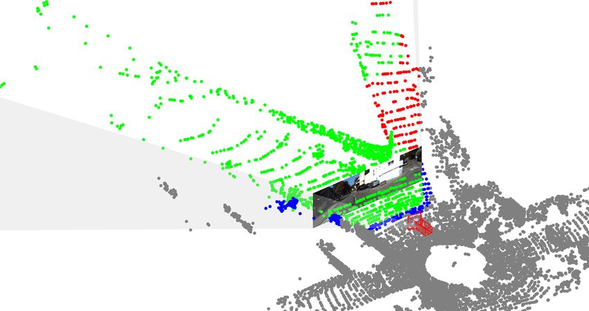
without explicit feature descriptors as illustrated in Fig. 1.   Point Cloud-to-Point Cloud Registration. The avail-
Our method requires lesser storage memory, i.e., O(3N )          ability of 3D information enables direct registration be-
for the reference point cloud since we do not rely on feature    tween point clouds without establishing feature correspon-
descriptors to establish correspondences. Furthermore, the       dences. Methods like ICP [2, 5], NDT [3] work well with
images captured by cameras can be directly utilized without      proper initial guess, and global optimization approaches
SfM. We solve the cross-modal image-to-point cloud regis-        such as Go-ICP [40] work without initialization require-
tration problem in two stages. In the first stage, we design     ments. These methods are widely used in point cloud based
a two-branch neural network that takes the image and point       SLAM algorithms like LOAM [45], Cartographer [18], etc.
cloud as inputs, and outputs a label for every point that in-    Recently data driven methods like DeepICP [24], Deep-
dicates whether the projection of this point is within or be-    ClosestPoint [39], RPM-Net [42], etc, are also proposed.
yond the image frustum. The second stage is formulated           Although these approaches do not require feature corre-
as an unconstrained continuous optimization problem. The         spondences, they still rely heavily on the geometrical de-
objective is to find the optimal camera pose, i.e., the rigid    tails of the point structures in the same modality to work
transformation with respect to the reference frame of the        well. Consequently, these approaches cannot be applied
point cloud, such that 3D points labeled as within the cam-      to our task on cross-modal registration. Another group of
era frustum is correctly projected into the image. Standard      common approaches is the two-step feature-based registra-
solvers such as the Gauss-Newton algorithm can be used to        tion. Classical point cloud feature detectors [36, 46, 32, 8]
solve our camera pose optimization problem. Extensive ex-        and descriptors [35, 31] usually suffer from noise and clut-
perimental results on the open-source Oxford Robotcar and        ter environments. Recently deep learning based feature
KITTI datasets show the feasibility of our approach.             detectors like USIP [22], 3DFeatNet [41], and descriptors
    The main contributions of this paper are listed as follow:   like 3DMatch [44], PPF-Net [7], PPF-FoldNet [6], Perfect-
                                                                 Match [15], have demonstrated improved performances in
   • We circumvent the challenging need to learn cross-          point cloud-based registration. Similar to image-to-image
     modal feature descriptor for registration by casting the    registration, these approaches require feature descriptors
     problem into a two-stage classification and optimiza-       that are challenging to obtain in cross-modality registration.
     tion framework.
   • A two-branch neural network with attention modules          Image-to-Point Cloud Registration. To the best of our
     to enhance cross-modality fusion is designed to learn       knowledge, 2D3D-MatchNet [11] is the only prior work
     labels of whether a 3D point is within or beyond the        for general image-point cloud registration. It extracts im-
     camera frustum.                                             ages keypoints with SIFT [23], and point cloud keypoints
   • The inverse camera projection optimization is pro-          with ISS [46]. The image and point cloud patches around
     posed to solve for the camera pose with the classifi-       the keypoints are fed into each branch of a Siamese-like
     cation labels of the 3D points.                             network and trained with triplet loss to extract cross-modal
                                                                 descriptors. At inference, it is a standard pipeline that con-
   • Our method and the experimental results show a
                                                                 sists of RANSAC-based descriptor matching and EPnP [20]
     proof-of-concept that cross-modal registration can be
                                                                 solver. Despite its greatly simplified experimental settings
     achieved with deep classification.
                                                                 where the point clouds and images are captured at nearby
                                                                 timestamps with almost zero relative rotation, the low in-
2. Related Works                                                 lier rate of correspondences reveals the struggle for a deep
Image-to-Image Registration. Images-to-image regis-              network to learn common features across the drastically
trations [34, 33] are done in the P2 space because of the        different modalities. Another work [43] establishes 2D-
lack of depth information. This is usually the first step to     3D line correspondences between images and prior Lidar
the computation of the projective transformation or SfM.         maps, but they requires accurate initialization, e.g., from a
Typical methods are usually based on feature matching. A         SLAM/Odometry system. In contrast, the general image-
set of features such as SIFT [23] or ORB [30] are extracted      to-point cloud registration, including 2D3D-MatchNet [11]
from both source and target images. Correspondences are          and our DeepI2P do not rely on another accurate localiza-
then established based on the extracted features, which can      tion system. Some other works [27, 4] focus on image-to-
be used to solve for the rotation, translation using Bundle      point cloud place recognition / retrieval without estimating
Adjustment [37, 16], Perspective-n-Point solvers [12], etc.      the relative rotation and translation.
Such techniques have been applied in modern SLAM sys-
tems [10, 26, 9]. However, such methods are based on fea-        3. Overview of DeepI2P
ture descriptors in the image modality to establish corre-
                                                                    We denote an image as I ∈ R3×W ×H , where W and H
spondences, and do not work for our general image-to-point
                                                                 are the image width and height, and a point cloud as P =
cloud registration task.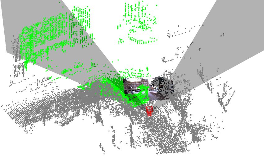
{P1 , P2 , · · · , PN | Pn ∈ R3 }. The cross-modal image-to-      Point Cloud Encoder. Given an input point cloud de-
point cloud registration problem is to solve for the rotation     noted as P ∈ R3×N , a set of nodes P(1) ∈ R3×M1 is
matrix R ∈ SO(3) and translation vector t ∈ R3 between            sampled by Farthest Point Sampling (FPS). A point-to-node
the coordinate frames of the camera and point cloud. The          grouping [21] is performed to obtain M1 clusters of points.
problem is difficult because standard approaches such as          Each cluster is processed by a PointNet [28] to get M1 fea-
ICP, PnP and Bundle Adjustment (BA) algorithms cannot             ture vectors of length C1 , respectively, i.e. P (1) ∈ RC1 ×M1 .
be used due to the lack of point-to-pixel correspondences.        The point-to-node grouping is adaptive to the density of
Unlike the point cloud obtained from SfM, our point cloud         points. This is beneficial especially for point clouds from
is obtained from a point cloud scanner and does not contain       Lidar scans, where points are sparse at far range and dense
any image-based feature descriptors. Establishing cross-          at near range. The above sampling-grouping-PointNet op-
modal point-to-pixel correspondence is non-trivial. This          eration is performed again to obtain another set of feature
is because the points in the R3 space shares very little ap-      vectors P (2) ∈ RC2 ×M2 . Finally, a PointNet is applied to
pearance and geometric correlations with the image in the         obtain the global point cloud feature vector P (3) ∈ RC3 ×1 .
P2 space. We circumvent the problem by designing our
cross-modality image-to-point cloud registration approach         Image-Point Cloud Attention Fusion. The goal of the
to work without point-to-pixel correspondences.                   classification is to determine whether a point projects to
    To this end, we propose a two-stage “Frustum classifica-      the image plane (frustum classification) and which region
tion + Inverse camera projection” pipeline. The first stage       it falls into (grid classification). Hence, it is intuitive that
classifies each point in the point cloud into within or beyond    the classification requires fusion of information from both
the camera frustum. We call this the frustum classification,      modalities. To this end, we design an Attention Fusion
which is done easily by a deep network shown in Section 4.        module to combine the image and point cloud information.
In the second stage, we show that it is sufficient to solve the   The input to the Attention Fusion module consists of three
pose between camera and point cloud using only the frus-          parts: a set of node features Patt (P (1) or P (2) ), a set of
tum classification result. This is the inverse camera projec-     image features Iatt ∈ RCimg ×Hatt ×Watt (I (1) or I (2) ), and
tion problem in Section 5.1. In our supplementary materi-         the global image feature vector I (3) . As shown in Fig. 2,
als, we propose another cross-modality registration method        the image global feature is stacked and concatenated with
“Grid classification + PnP” as our baseline for experimental      the node features Patt , and fed into a shared MLP to get
comparison. In the grid classification, the image is divided      the attention score Satt ∈ RHatt Watt ×M . Satt provides
into a tessellation of smaller regular grids, and we predict      a weighting of the image features Iatt for M nodes. The
the cell each 3D point projects into. The pose estimation         weighted image features are obtained by multiplying Iatt
problem can then be solved by applying RANSAC-based               and Satt . The weighted image features can now be concate-
PnP to the grid classification output.                            nated with the node features in the point cloud decoder.

                                                                  Point Cloud Decoder. The decoder takes the image and
4. Classification                                                 point cloud features as inputs, and outputs the per-point
   The input to the network is a pair of image I and point        classification result. In general, it follows the interpolation
cloud P , and the output is a per-point classification for        idea of PointNet++ [29]. At the beginning of the decoder,
P . There are two classification branches: frustum and grid       the global image feature I (3) and global point cloud fea-
classification. The frustum classification assign a label to      ture P (3) are stacked M2 times, so that they can be con-
each point, Lc = {l1c , l2c , · · · , lN
                                       c
                                         }, where lnc ∈ {0, 1}.   catenated with the node features P (2) and the Attention Fu-
 c
ln = 0 if the point Pn is projected to outside the image          sion output I˜(2) . The concatenated [I (3) , I˜(2) , P (3) , P (2) ] is
I, and vice versa. Refer to the supplementary for the details     processed by a shared MLP to get M2 feature vectors de-
of the grid classification branch used in our baseline.           noted as P̃ (2) ∈ RC2 ×M2 . We perform interpolation to get
                                                                    (2)
                                                                  P̃(itp) ∈ RC2 ×M1 , where the M2 features are upsampled to
4.1. Our Network Design                                           M1 ≥ M2 features. Note that P (2) and P̃ (2) are associated
                                                                  with node coordinates P(2) ∈ R3×M2 . The interpolation
   As shown in Fig. 2, our per-point classification network
                                                                  is based on k-nearest neighbors between node coordinates
consists of four parts: point cloud encoder, point cloud de-
                                                                  P(1) ∈ R3×M1 , where M1 ≥ M2 . For each C2 channel,
coder, image encoder and image-point cloud attention fu-
                                                                  the interpolation is denoted as:
sion. The point cloud encoder/decoder follows the design
of SO-Net [21] and PointNet++ [29], while the image en-                            Pk          (2)
                                                                      (2)           j=1   wj P̃j                             1
coder is a ResNet-34 [17]. The classified points are then           P̃(itp)i   =    Pk               , where wj =                     ,
                                                                                                                        (1)  (2)
used in our inverse camera projection optimization in Sec-                              j=1   wj                     d(Pi , Pj )
tion 5.1 to solve for the unknown camera pose.                                                                                        (1)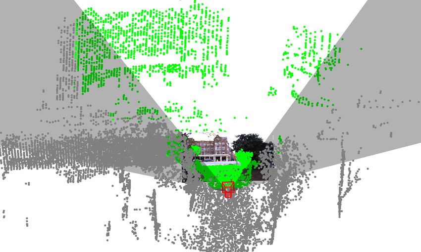
Frustum
Classification
Shared MLP
Shared MLP
Shared MLP
Interpolation
Interpolation
FPS&Group
FPS&Group
Gloabl PC
PointNet
PointNet
PointNet
Feature
Attention Attention
Fusion Fusion
Grid
Classification
AvgPool
ResNet
ResNet
Gloabl Img
Legend
Feature
PC Encoder
PC Decoder
Img Encoder
Stacked
Weighted Image Features
Shared MLP
Attention
PC node for each node
Fusion
Feature
...
Attention scores
Figure 2. Our network architecture for the classification problem.
(2) (1)
and Pj is one of the k-nearest neighbors of Pi in P(2) . Frustum Classification. For a given camera pose G, we
We get
(2)
P̃(itp) ∈R C2 ×M1
with the concatenate-sharedMLP- define the function:
(1)
interpolation process. Similarly, we obtain P̃(itp) ∈ RC1 ×N f (Pi ; G, K, H, W ) =
after another round of operations. Lastly, we obtain the final
(
1 : 0 ≤ p0xi ≤ W − 1, 0 ≤ p0yi ≤ H − 1, zi0 > 0 (5)
output (2 + HW/(32 × 32)) × N , which can be reorganized ,
0 : otherwise
into the frustum prediction scores 2 × N and grid prediction
scores (HW/(32 × 32)) × N . which assigns a label of 1 to a point Pi that projects within
4.2. Training Pipeline the image, and 0 otherwise. Now the frustum classifica-
tion labels are generated as lic = f (Pi ; G, K, H, W ), where
The generation of the frustum labels is simply a camera G is known during training. In the Oxford Robotcar and
projection problem. During training, we are given the cam- KITTI datasets, we randomly select a pair of image and raw
era intrinsic matrix K ∈ R3×3 and the pose G ∈ SE(4) point cloud (I, Praw ), and compute the relative pose from
between the camera and point cloud. The 3D transforma- the GPS/INS readings as the ground truth pose Gpc . We use
tion of a point Pi ∈ R3 from the point cloud coordinate (I, Praw ) with a relative distance within a specified interval
frame to the camera coordinate frame is given by: in our training data. However, we observe that the rota-
" #" # tions in Gpc are close to zero from the two datasets since
R t Pi
P̃0i = [Xi0 , Yi0 , Zi0 , 1]> = GP̃i = , (2) the cars used to collect the data are mostly undergoing pure
0 1 1 translations. To avoid overfitting to such scenario, we apply
randomly generated rotations Gr onto the raw point cloud
and the point P̃0i is projected into the image coordinate:
to get the final point cloud P = Gr Praw in the training
0
xi
fx 0 cx
data. Furthermore, the ground truth pose is now given by
p̃0i = yi0 = KP0i = 0
fy cy P0i .
(3) G = Gpc G−1 r . Note that random translation can also be in-
cluded in Gr , but it does not have any effect on the training
zi0 0 0 1
since the network is translational equivariant.
Note that homogeneous coordinate is represented by a tilde
symbol, e.g., P̃0i is the homogeneous representation of P0i . Training Procedure. The frustum classification training
The inhomogeneous coordinate of the image point is: procedure is summarized as:
p0i = [p0xi , p0yi ]> = [x0i /zi0 , yi0 /zi0 ]> . (4) 1. Select a pair of image and point cloud (I, Praw ) with
relative pose Gpc .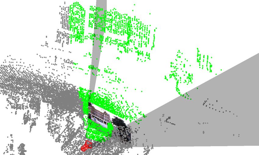
2. Generate 3D random transformation Gr , and apply it               Frustum Prediction Equals to 0. We now consider a
     to get P = Gr Praw and G = Gpc G−1        r .                     point Pi with prediction ˆlic = 0. The cost defined along
  3. Get the ground truth per-point frustum labels lic ac-             the image x-axis is given by:
     cording to Eq. 5.
  4. Feed (I, P ) into the network illustrated in Fig. 2.                                                    W          W
                                                                                       u(p0xi ; W ) =          − p0xi −   .               (9)
  5. Frustum prediction L̂c = {ˆl1c , · · · , ˆlnc }, ˆlic ∈ {0, 1}.                                         2          2
  6. Apply cross entropy loss for the classification tasks to
     train the network.                                                It is negative when p0xi falls outside the borders along the
                                                                       image width, and positively proportional to the distance to
5. Pose Optimization                                                   the closest border along the image x-axis otherwise. Simi-
                                                                       larly, an analogous cost u(p0yi ; H) along the y-axis can be
     We now formulate an optimization method to get the
                                                                       defined. Furthermore, an indicator function:
pose of the camera in the point cloud reference frame with
the frustum classification results. Note that we do not use                                             max(u(p0xi ; W ), 0)
deep learning in this step since the physics and geometry of              1(p0xi , p0yi , zi0 ; H, W ) =
                                                                                                              u(p0xi ; W )
the camera projection model is already well-established.                                                  0                             (10)
     Formally, the pose optimization problem is to solve for                                      max(u(pyi ; H), 0) max(zi0 , 0)
                                                                                                ·                      ·
Ĝ, given the point cloud P , frustum predictions L̂c =                                              u(p0yi ; H)           zi0
{ˆl1c , · · · , ˆlN
                  c
                    }, ˆlic ∈ {0, 1}, and camera intrinsic matrix K.
In this section, we describe our inverse camera projection             is required to achieve the target of zero cost when p0i is out-
solver to solve for Ĝ.                                                side the H × W image or P0i is behind the camera (i.e.
                                                                       zi0 < 0).
5.1. Inverse Camera Projection
                                                                       Cost Function. Finally, the cost function for a single
   The frustum classification of a point, i.e., Lc given G de-         point Pi is given by:
fined in Eq. 5 is based on the forward projection of a cam-                                     (
era. The inverse camera projection problem is the other way                                       ri0 : ˆlic = 0
around, i.e, determine the optimal pose Ĝ that satisfies a                      ri (G; ˆli ) =
                                                                                          c
                                                                                                                 , where (11)
                                                                                                  ri1 : ˆlic = 1
given L̂c . It can be written more formally as:
                 N
                 X                                                       ri0 = (u(p0xi ; W ) + u(p0yi ; H)) · 1(p0xi , p0yi , zi0 ; H, W ),
                      f (Pi ; G, K, H, W ) − 0.5 ˆ
                                                 c
 Ĝ = arg max                                     li − 0.5 . (6)
        G∈SE(3) i=1                                                      ri1 = g(p0xi ; W ) + g(p0yi ; H) + h(zi0 ).
Intuitively, we seek to find the optimal pose Ĝ such that all         p0xi , p0yi , zi are functions of G according to Eq. 2, 3 and
3D points with label ˆlic = 1 from the network are projected           4. Image height H, width W and camera intrinsics K are
into the image, and vice versa. However, a naive search of             known. Now the optimization problem in Eq. 6 becomes:
the optimal pose in the SE(3) space is intractable. To mit-                                                    n
igate this problem, we relax the cost as a function of the
                                                                                                               X
                                                                                         Ĝ = arg min              ri (G; ˆlic )2 .     (12)
distance from the projection of a point to the image bound-                                       G∈SE(3) i=1
ary, i.e., a H × W rectangle.
                                                                       This is a typical unconstrained least squares optimization
Frustum Prediction Equals to 1. Let us consider a point
                                                                       problem. We need proper parameterization of the unknown
Pi with the prediction ˆlic = 1. We define cost function:
                                                                       transformation matrix,
    g(p0xi ; W ) = max(−p0xi , 0) + max(p0xi − W, 0)            (7)                     "            #
                                                                                            R    t
                                                                                  G=                     , with R ∈ SO(3), t ∈ R3 ,      (13)
that penalizes a pose G which causes p0xi of the projected                                  0    1
point p0i = [p0xi , p0yi ]> (c.f. Eq. 4) to fall outside the borders
of the image width. Specifically, the cost is zero when p0xi is        where G ∈ SE(3) is an over-parameterization that can
within the image width, and negatively proportional to the             cause problems in the unconstrained continuous optimiza-
distance to the closest border along the image x-axis other-           tion. To this end, we use the Lie-algebra representation ξ ∈
wise. A cost g(p0yi ; H) can be analogously defined along              se(3) for the minimal parameterization of G ∈ SE(3). The
image y-axis. In addition, cost function h(·) is defined to            exponential map G = expse(3) (ξ) converts se(3) 7→ SE(3),
avoid the ambiguity of P0i falling behind the camera:                  while the log map ξ = logSE(3) (G) converts SE(3) 7→
                                                                       se(3). Similar to [10], we define the se(3) concatenation
                   h(zi0 ) = α · max(−z 0 , 0),                 (8)    operator ◦ : se(3) × se(3) 7→ se(3) as:
where α is a hyper-parameter that balances the weighting
                                                                        ξki = ξkj ◦ ξji = logSE(3) expse(3) (ξkj ) · expse(3) (ξji ) , (14)
between g(·) and h(·).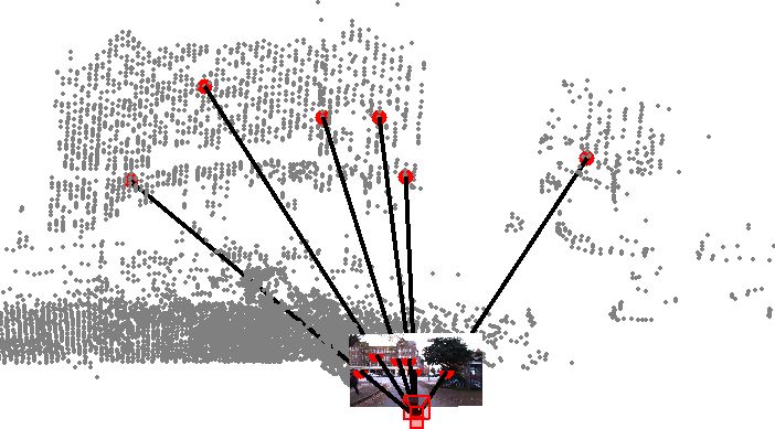
and the cost function in Eq. 12 can be re-written with the                  clouds in KITTI suffers from severe occlusion, sparse mea-
proper exponential or log map modifications into:                           surement at far range, etc. More details of the two dataset
                                                                            configurations are in the supplementary materials.
                     ˆ
      Ĝ = expse(3) (ξ),    where
                                      n
                                      X                            (15)     6.1. Implementation Details
      ξˆ = arg min krk2 = arg min            ri (ξ; ˆlic )2 .
               ξ                 ξ                                          Classification Network. Refer to our supplementary ma-
                                       i=1
                                                                            terials for the network implementation details. These in-
Gauss-Newton Optimization. Eq. 15 is a typical least                        cludes parameters of the PointNet and SharedMLP mod-
squares optimization problem that can be solved by the                      ules, number of nodes in P(1) , P(2) , number of nearest
Gauss-Newton method. During iteration i with the current                    neighbor k for point cloud interpolation in the decoder, etc.
solution ξ (i) , the increment δξ (i) is estimated by a Gauss-
Newton second-order approximation:                                          Inverse Camera Projection. The initial guess G(0) in our
                                                                            proposed inverse camera projection (c.f. Section 5.1) is
                                                 ∂r( ◦ ξ (i) )
 δξ (i) = −(J > J)−1 J > r(ξ (i) ), where J =                           ,   critical since the solver for Eq. 15 is an iterative approach.
                                                     ∂           =0
                                                                   (16)     To alleviate the initialization problem, we perform the op-
and the update is given by ξ (i+1) = δξ (i) ◦ ξ (i) . Finally the           timization 60 times with randomly generated initialization
inverse camera projection problem is solved by performing                   G(0) , and select the solution with the lowest cost. In ad-
the exponential map Ĝ = expse(3) (ξ).ˆ A visualization of                  dition, the 6DoF search space is too large for random ini-
our iterative optimization is presented in Fig. 3.                          tialization. We mitigate this problem by leveraging on the
                                                                            fact that our datasets are from ground vehicles to perform
6. Experiments                                                              random initialization in 2D instead. Specifically, R(0) is
                                                                            initialized as a random rotation around the up-axis, and t(0)
   Our image-to-point cloud registration approach is evalu-                 as a random translation in the x-y horizontal plane. Our
ated with Oxford Robotcar [25] and KITTI [13] dataset.                      algorithm is implemented with Ceres [1].
Oxford dataset. The point clouds are built from the ac-
                                                                            6.2. Registration Accuracy
cumulation of the 2D scans from a 2D Lidar. Each point
cloud is set at the size of radius 50m, i.e. diameter 100m.                    The frustum classification accuracy is 98% and 94% on
The images are captured by the center camera of a Bumble-                   the Oxford and KITTI dataset, respectively. However, these
bee tri-camera rig. Similar to 3DFeat-Net [41], 35 traver-                  numbers does not translate directly to the registration accu-
sals are used for training, while 5 traversals are for testing.             racy. Following the practice of [22, 41], the registration is
In training and inference, the image-point cloud pair is se-                evaluated with two criteria: average Relative Translational
lected using the following steps: a) Choose a Lidar point                   Error (RTE) and average Relative Rotation Error (RRE).
cloud from one of the traversals. b) Randomly select an                     The results are shown in Table 1 and Fig. 4.
image from the same traversal and captured within ±10m                         Grid Cls. + PnP is the result of our “Grid classification
from the coordinate origin of the point cloud. The relative                 + PnP” baseline method (see Supplementary materials for
pose of the camera to the point cloud coordinate frame is                   details). The RANSAC PnP algorithm optimizes the full
Gpc . c) Apply a random 2D rotation (around the up-axis)                    6-DoF Ĝ without any constraints. Frus. Cls. + Inv.Proj.
and translation (along the x-y plane) Gr to the point cloud.                represents the result of our “Frustum classification + Inverse
d) The objective is to recover the ground truth transforma-                 camera projection” method. The difference between Frus.
tion Ggt = Gpc G−1 r . There are 130,078 point clouds for                   Cls. + Inv.Proj. 3D and Frus. Cls. + Inv.Proj. 2D is that
training and 19,156 for testing.                                            the former is optimizing the full 6-DoF Ĝ, while the latter
KITTI Odometry dataset. Point clouds are directly ac-                       constrains Ĝ to be 3-DOF, i.e., translation on x-y horizontal
quired from a 3D Lidar. The image-point cloud pairs are se-                 plane and rotation around the up-axis.
lected in a similar way to that in Oxford dataset, i.e., a pair                Due to the lack of existing approaches in solving the
of image and point cloud is captured within ±10m. The im-                   image-to-point cloud registration problem under the same
ages are from both the left and right cameras that are facing               setting, we further compare our DeepI2P with 4 other ap-
the front. We follow the common practice of utilizing the 0-                proaches that may contain unfair advantages over ours in
8 sequences for training, and 9-10 for testing. In total there              their input data modality or configurations.
are 20,409 point clouds for training, and 2,792 for testing.                1) Direct Regression uses a deep network to directly
Remarks: Note that a KITTI point cloud is from a single                     regress the relative poses. It consists of the Point Cloud
frame 3D Lidar scan, while an Oxford point cloud is an ac-                  Encoder and Image Encoder in Section 4. The global point
cumulation of 2D Lidar scans over 100m. As a result, point                  cloud feature and global image feature are concatenated into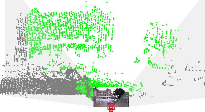
Figure 3. Visualizations of the Gauss-Newton at iteration 0 / 40 / 80 from left to right. Green points are classified as inside image FoV.
                                      Table 1. Registration accuracy on the Oxford and KITTI datasets.
                                                              Oxford                               KITTI
                                                    RTE (m)         RRE (◦ )             RTE (m)         RRE (◦ )
          Direct Regression                        5.02 ± 2.89 10.45 ± 16.03            4.94 ± 2.87 21.98 ± 31.97
          MonoDepth2 [14] + USIP [22]              33.2 ± 46.1 142.5 ± 139.5            30.4 ± 42.9 140.6 ± 157.8
          MonoDepth2 [14] + GT-ICP                  1.3 ± 1.5       6.4 ± 7.2            2.9 ± 2.5    12.4 ± 10.3
          2D3D-MatchNet [11] (No Rot§ )                1.41           6.40                  NA            NA
          Grid Cls. + PnP                          1.91 ± 1.56 5.94 ± 10.72             3.22 ± 3.58 10.15 ± 13.74
          Frus. Cls. + Inv.Proj. 3D                2.27 ± 2.19 15.00 ± 13.64            3.17 ± 3.22 15.52 ± 12.73
          Frus. Cls. + Inv.Proj. 2D                1.65 ± 1.36    4.14 ± 4.90           3.28 ± 3.09   7.56 ± 7.63
                        §
                            Point clouds are not randomly rotated in the experiment setting of 2D3D-MatchNet [11].

a single vector and processed by a MLP that directly re-
gresses Ĝ. See the supplementary materials for more de-
tails of this method. Table 1 shows that our DeepI2P signif-
icantly outperforms the simple regression method.
2) Monodepth2+USIP converts the cross-modality regis-
                                                                          Figure 4. Histograms of image-point cloud registration RTE and
tration problem into point cloud-based registration by using
                                                                          RRE on the Oxford and KITTI datasets. x-axis is RTE (m) and
Monodepth2 [14] to estimate a depth map from a single im-
                                                                          RRE (◦ ), and y-axis is the percentage.
age. The Lidar point cloud is used to calibrate the scale of
depth map from MonoDepth2, i.e. the scale of the depth                    trast, the point clouds in our experiments are always ran-
map is perfect. Subsequently, the poses between the depth                 domly rotated. This means 2D3D-MatchNet is solving a
map and point cloud are estimated with USIP [22]. This is                 much easier problem, but their results are worse than ours.
akin to same modality point cloud-to-point cloud registra-
tion. Nonetheless, Table 1 shows that this approach under-                Distribution of Errors. The distribution of the registra-
performs. This is probably because the depth map is inac-                 tion RTE (m) and RRE (◦ ) on the Oxford and KITTI dataset
curate and USIP does not generalize well on depth maps.                   are shown in Fig. 4. It can be seen that our performance
                                                                          is better on Oxford than KITTI. Specifically, the mode of
3) Monodepth2+GT-ICP acquires a depth map with ab-                        the translational/rotational errors are ∼ 1.5m/3◦ on Oxford
solute scale in the same way as Monodepth2+USIP. How-                     and ∼ 2m/5◦ on KITTI. The translational/rotational error
ever, it uses Iterative Closest Point (ICP) [2, 5] to estimate            variances are also smaller on Oxford.
the pose between the depth map and point cloud. Note that
ICP fails without proper initialization, and thus we use the              Acceptance of RTE/RRE. There are other same-
ground truth (GT) relative pose for initialization. Table 1               modality methods that solves registration on Oxford and
shows that our DeepI2P achieves similar RTE and better                    KITTI dataset, e.g. USIP [22] and 3DFeatNet [41] that
RRE compared to Monodepth2+GT-ICP, despite the latter                     gives much better RTE and RRE. These methods work
has the unfair advantages of ground truth initialization and              only on point cloud-to-point cloud instead of image-to-
the depth map is perfectly calibrated.                                    point cloud data, and thus are not directly comparable to our
                                                                          method. Furthermore, we note that the reported accuracy of
4)2D3D-MatchNet [11] is the only prior work for cross-                    our DeepI2P in Table 1 is sufficient for non life-critical ap-
modal image-to-point cloud registration to our best knowl-                plications such as frustum localization of mobile devices in
edge. However, the rotation between camera and Lidar is                   both indoor and outdoor environments.
almost zero in their experiment setting. This is because the
images and point clouds are taken from temporally consec-                 Oxford vs KITTI. Our performance on Oxford is better
utive timestamps without additional augmentation. In con-                 than on KITTI for several reasons: 1) The point clouds in
Oxford are built from 2D scans accumulated over 100m Table 2. Registration accuracy on Oxford
from a Lidar scanner, while KITTI point cloud is a single # points # init. t limit RTE RRE
scan from a 3D Lidar as shown in Fig. 6. Consequently, the DeepI2P 20480 60 10 1.65 4.14
occlusion effect in KITTI is severe. For example, the image DeepI2P 20480 30 10 1.81 4.37
captured in timestamp tj is seeing things that are mostly DeepI2P 20480 10 10 2.00 4.56
DeepI2P 20480 1 10 3.52 5.34
occluded/unobserved from the point cloud of timestamp ti .
DeepI2P 20480 60 5 1.52 3.30
Given the limited Field-of-View (FoV) of the camera, the
DeepI2P 20480 60 15 1.96 4.74
cross-modality registration becomes extremely challenging
DeepI2P 10240 60 10 1.80 4.35
since two modalities are observing different scene contents.
DeepI2P 5120 60 10 1.94 4.63
2) The vertical field-of-view of the point clouds in KITTI DeepI2P noAtten. 20480 60 10 6.88 20.93
is very limited, which leads to lack of distinctive verti- MonoDepth2+ICP 20480 60 10 8.45 75.54
cal structures for cross-modality matching. Most of the
points on the ground are structureless and thus not useful
for matching across modalities. 3) “KITTI Odometry” is
a small dataset that contains only 20,409 point clouds for
training, while Oxford is ∼ 6.4× larger with 130,078 point
clouds. As a result, we observe severe network overfitting
in the KITTI dataset but not in the Oxford dataset.
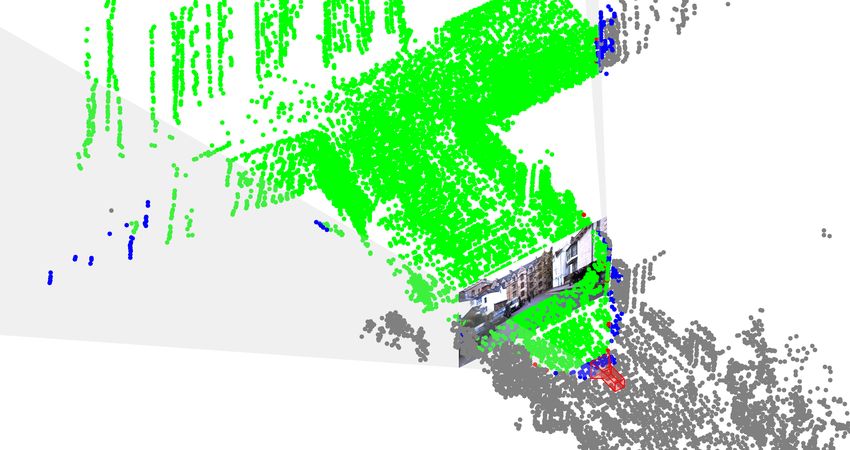
Figure 5. Visualization of the frustum and grid classification re-
6.3. Ablation Study sults projected onto the images. Green - both frustum and grid
predictions are correct. Yellow - frustum prediction is correct but
Initialization of our Gaussian-Newton and Mon- grid prediction is wrong. Red - frustum prediction is outside image
odepth2+ICP. In the 2D registration setting, there are 3 FoV, but ground truth label is inside FoV. Blue - frustum predic-
unknown parameters - rotation θ, translation tx , ty . For our tion is inside image FoV, but ground truth label is outside FoV.
method, the initial θ is easily obtained by aligning the av- Best view in color and zoom-in.
erage yaw-angles of the predicted in-frustum points with
the camera principle axis. Therefore, our 60-fold initializa-
tion is only for two-dimensional search for tx , ty . In con-
trast, Monodepth2+ICP requires three-dimensional search
for θ, tx , ty . As shown in Tab. 2, our DeepI2P is robust to
initialization, while Monodepth2+ICP performs a lot worse Figure 6. 3D Visualization of the frustum classification and inverse
with 60-fold random initialization. camera projection on the Oxford (Left) and KITTI (Right).
In-image occlusion. In Oxford/Kitti, occlusion effect can
accuracy of the frustum and grid classifications are around
be significant when the translation is large, e.g. > 5m.
98% and 51% in Oxford, and 94% and 39% in KITTI. The
Tab. 2 shows that the registration improves when the maxi-
low classification accuracy in KITTI leads to larger RTE
mum translation limit decrease (15m → 10m → 5m).
and RRE during cross-modality registration. 3D visualiza-
Cross-attention module. Tab. 2 shows the significant tion of the frustum classification and the inverse camera pro-
drop in registration accuracy w/o cross-attention module. jection problem is illustrated in Fig. 6. It illustrates the intu-
Additionally, we also see the coarse classification accuracy ition that a camera pose can be found by aligning the camera
drops significantly from 98% to 80%. frustum to the classification result.
3D point density. As shown in Tab. 2, our registration ac- 7. Conclusions
curacy decreases with reducing point density. Nonetheless,
the performance drop is reasonable even when the point The paper proposes an approach for cross-modality reg-
density drops to 1/4 (20480 → 5120). istration between images and point clouds. The challenging
registration problem is converted to a classification problem
6.4. Visualizations solved by deep networks and an inverse camera projection
problem solved by least squares optimization. The feasibil-
Fig. 5 shows examples of the results from our frustum
ity of our proposed classification-optimization framework
classification network and the baseline grid classification
is verified with Oxford and KITTI dataset.
network (see supplementary materials). The point clouds
are projected into the images using the ground truth pose Acknowledgment. This work is supported in part by the
G. The colors of the points represent the correctness of the Singapore MOE Tier 1 grant R-252-000-A65-114.
frustum or grid predictions as described in the caption. TheReferences [15] Zan Gojcic, Caifa Zhou, Jan D Wegner, and Andreas Wieser.
The perfect match: 3d point cloud matching with smoothed
[1] Sameer Agarwal, Keir Mierle, and Others. Ceres solver. densities. In Proceedings of the IEEE Conference on Com-
http://ceres-solver.org. puter Vision and Pattern Recognition, pages 5545–5554,
[2] Paul J Besl and Neil D McKay. Method for registration of 2019.
3-d shapes. In Sensor fusion IV: control paradigms and data [16] Richard Hartley and Andrew Zisserman. Multiple view ge-
structures, volume 1611, pages 586–606. International Soci- ometry in computer vision. Cambridge university press,
ety for Optics and Photonics, 1992. 2003.
[3] Peter Biber and Wolfgang Straßer. The normal distribu- [17] Kaiming He, Xiangyu Zhang, Shaoqing Ren, and Jian Sun.
tions transform: A new approach to laser scan matching. Deep residual learning for image recognition. In Proceed-
In Proceedings 2003 IEEE/RSJ International Conference ings of the IEEE conference on computer vision and pattern
on Intelligent Robots and Systems (IROS 2003)(Cat. No. recognition, pages 770–778, 2016.
03CH37453), volume 3, pages 2743–2748. IEEE, 2003. [18] Wolfgang Hess, Damon Kohler, Holger Rapp, and Daniel
[4] Daniele Cattaneo, Matteo Vaghi, Simone Fontana, Au- Andor. Real-time loop closure in 2d lidar slam. In 2016
gusto Luis Ballardini, and Domenico Giorgio Sorrenti. IEEE International Conference on Robotics and Automation
Global visual localization in lidar-maps through shared 2d- (ICRA), pages 1271–1278. IEEE, 2016.
3d embedding space. In 2020 IEEE International Confer- [19] Laurent Kneip, Hongdong Li, and Yongduek Seo. Upnp: An
ence on Robotics and Automation (ICRA), pages 4365–4371. optimal o (n) solution to the absolute pose problem with uni-
IEEE, 2020. versal applicability. In European Conference on Computer
[5] Yang Chen and Gérard Medioni. Object modelling by regis- Vision, pages 127–142. Springer, 2014.
tration of multiple range images. Image and vision comput- [20] Vincent Lepetit, Francesc Moreno-Noguer, and Pascal Fua.
ing, 10(3):145–155, 1992. Epnp: An accurate o (n) solution to the pnp problem. Inter-
[6] Haowen Deng, Tolga Birdal, and Slobodan Ilic. Ppf-foldnet: national journal of computer vision, 81(2):155, 2009.
Unsupervised learning of rotation invariant 3d local descrip- [21] Jiaxin Li, Ben M Chen, and Gim Hee Lee. So-net: Self-
tors. In Proceedings of the European Conference on Com- organizing network for point cloud analysis. In Proceed-
puter Vision (ECCV), pages 602–618, 2018. ings of the IEEE conference on computer vision and pattern
[7] Haowen Deng, Tolga Birdal, and Slobodan Ilic. Ppfnet: recognition, pages 9397–9406, 2018.
Global context aware local features for robust 3d point [22] Jiaxin Li and Gim Hee Lee. Usip: Unsupervised stable in-
matching. In Proceedings of the IEEE Conference on Com- terest point detection from 3d point clouds. In Proceedings
puter Vision and Pattern Recognition, pages 195–205, 2018. of the IEEE International Conference on Computer Vision,
[8] Chitra Dorai and Anil K. Jain. Cosmos-a representation pages 361–370, 2019.
scheme for 3d free-form objects. IEEE Transactions on Pat- [23] David G Lowe. Object recognition from local scale-invariant
tern Analysis and Machine Intelligence, 19(10):1115–1130, features. In Proceedings of the seventh IEEE international
1997. conference on computer vision, volume 2, pages 1150–1157.
[9] Jakob Engel, Vladlen Koltun, and Daniel Cremers. Direct Ieee, 1999.
sparse odometry. IEEE transactions on pattern analysis and [24] Weixin Lu, Guowei Wan, Yao Zhou, Xiangyu Fu, Pengfei
machine intelligence, 40(3):611–625, 2017. Yuan, and Shiyu Song. Deepicp: An end-to-end deep neu-
[10] Jakob Engel, Thomas Schöps, and Daniel Cremers. Lsd- ral network for 3d point cloud registration. arXiv preprint
slam: Large-scale direct monocular slam. In European con- arXiv:1905.04153, 2019.
ference on computer vision, pages 834–849. Springer, 2014. [25] Will Maddern, Geoffrey Pascoe, Chris Linegar, and Paul
[11] Mengdan Feng, Sixing Hu, Marcelo H Ang, and Gim Hee Newman. 1 year, 1000 km: The oxford robotcar dataset.
Lee. 2d3d-matchnet: Learning to match keypoints across The International Journal of Robotics Research, 36(1):3–15,
2d image and 3d point cloud. In 2019 International Confer- 2017.
ence on Robotics and Automation (ICRA), pages 4790–4796. [26] Raul Mur-Artal, Jose Maria Martinez Montiel, and Juan D
IEEE, 2019. Tardos. Orb-slam: a versatile and accurate monocular slam
[12] Martin A Fischler and Robert C Bolles. Random sample system. IEEE transactions on robotics, 31(5):1147–1163,
consensus: a paradigm for model fitting with applications to 2015.
image analysis and automated cartography. Communications [27] Quang-Hieu Pham, Mikaela Angelina Uy, Binh-Son Hua,
of the ACM, 24(6):381–395, 1981. Duc Thanh Nguyen, Gemma Roig, and Sai-Kit Yeung. Lcd:
[13] Andreas Geiger, Philip Lenz, Christoph Stiller, and Raquel learned cross-domain descriptors for 2d-3d matching. In
Urtasun. Vision meets robotics: The kitti dataset. The Inter- Proceedings of the AAAI Conference on Artificial Intelli-
national Journal of Robotics Research, 32(11):1231–1237, gence, volume 34, pages 11856–11864, 2020.
2013. [28] Charles R Qi, Hao Su, Kaichun Mo, and Leonidas J Guibas.
[14] Clément Godard, Oisin Mac Aodha, Michael Firman, and Pointnet: Deep learning on point sets for 3d classification
Gabriel J Brostow. Digging into self-supervised monocular and segmentation. In Proceedings of the IEEE conference
depth estimation. In Proceedings of the IEEE international on computer vision and pattern recognition, pages 652–660,
conference on computer vision, pages 3828–3838, 2019. 2017.[29] Charles Ruizhongtai Qi, Li Yi, Hao Su, and Leonidas J Learning local geometric descriptors from rgb-d reconstruc-
Guibas. Pointnet++: Deep hierarchical feature learning on tions. In Proceedings of the IEEE Conference on Computer
point sets in a metric space. In Advances in neural informa- Vision and Pattern Recognition, pages 1802–1811, 2017.
tion processing systems, pages 5099–5108, 2017. [45] Ji Zhang and Sanjiv Singh. Loam: Lidar odometry and map-
[30] Ethan Rublee, Vincent Rabaud, Kurt Konolige, and Gary ping in real-time. In Robotics: Science and Systems, vol-
Bradski. Orb: An efficient alternative to sift or surf. In 2011 ume 2, 2014.
International conference on computer vision, pages 2564– [46] Yu Zhong. Intrinsic shape signatures: A shape descriptor for
2571. Ieee, 2011. 3d object recognition. In 2009 IEEE 12th International Con-
[31] Radu Bogdan Rusu, Nico Blodow, and Michael Beetz. Fast ference on Computer Vision Workshops, ICCV Workshops,
point feature histograms (fpfh) for 3d registration. In 2009 pages 689–696. IEEE, 2009.
IEEE international conference on robotics and automation,
pages 3212–3217. IEEE, 2009.
[32] Radu Bogdan Rusu and Steve Cousins. 3d is here: Point
cloud library (pcl). In 2011 IEEE international conference
on robotics and automation, pages 1–4. IEEE, 2011.
[33] Torsten Sattler, Bastian Leibe, and Leif Kobbelt. Improving
image-based localization by active correspondence search.
In European conference on computer vision, pages 752–765.
Springer, 2012.
[34] Yoli Shavit and Ron Ferens. Introduction to cam-
era pose estimation with deep learning. arXiv preprint
arXiv:1907.05272, 2019.
[35] Federico Tombari, Samuele Salti, and Luigi Di Stefano.
Unique signatures of histograms for local surface descrip-
tion. In European conference on computer vision, pages
356–369. Springer, 2010.
[36] Federico Tombari, Samuele Salti, and Luigi Di Stefano. Per-
formance evaluation of 3d keypoint detectors. International
Journal of Computer Vision, 102(1-3):198–220, 2013.
[37] Bill Triggs, Philip F McLauchlan, Richard I Hartley, and An-
drew W Fitzgibbon. Bundle adjustment—a modern synthe-
sis. In International workshop on vision algorithms, pages
298–372. Springer, 1999.
[38] Shimon Ullman. The interpretation of structure from mo-
tion. Proceedings of the Royal Society of London. Series B.
Biological Sciences, 203(1153):405–426, 1979.
[39] Yue Wang and Justin M Solomon. Deep closest point: Learn-
ing representations for point cloud registration. In Proceed-
ings of the IEEE International Conference on Computer Vi-
sion, pages 3523–3532, 2019.
[40] Jiaolong Yang, Hongdong Li, and Yunde Jia. Go-icp: Solv-
ing 3d registration efficiently and globally optimally. In Pro-
ceedings of the IEEE International Conference on Computer
Vision, pages 1457–1464, 2013.
[41] Zi Jian Yew and Gim Hee Lee. 3dfeat-net: Weakly su-
pervised local 3d features for point cloud registration. In
European Conference on Computer Vision, pages 630–646.
Springer, 2018.
[42] Zi Jian Yew and Gim Hee Lee. Rpm-net: Robust point
matching using learned features. In Conference on Computer
Vision and Pattern Recognition (CVPR), 2020.
[43] Huai Yu, Weikun Zhen, Wen Yang, Ji Zhang, and Sebas-
tian Scherer. Monocular camera localization in prior li-
dar maps with 2d-3d line correspondences. arXiv preprint
arXiv:2004.00740, 2020.
[44] Andy Zeng, Shuran Song, Matthias Nießner, Matthew
Fisher, Jianxiong Xiao, and Thomas Funkhouser. 3dmatch:A. “Grid Classification + PnP” Method problem after resizing the image into 1/32 of the original
size. Accordingly, the camera intrinsics K 0 after the resize
A.1. Grid Classification is obtained by dividing fx , fy , cx , cy with 32. There are
We divide the H ×W image into a tessellation of 32×32 many off-the-shelf PnP solver like EPnP [20], UPnP [19],
regions and then assign a label to each region. For exam- etc. We apply RANSAC on EPnP provided by OpenCV to
ple, an 128 × 512 image effectively becomes 4 × 16 = 64 robustly solve for Ĝ.
patches, and the respective regions are assigned to take
a label lf ∈ {0, 1, · · · , 63}. In the per-point classifica- Implementation details. The RANSAC PnP [12] from
tion, a point taking a label lf projects to the image re- OpenCV does not require initialization. We set the thresh-
gion with the same label. Consequently, the grid classi- old for inlier reprojection error to 0.6 and maximum itera-
fication is actually downsampling the image by a factor tion number to 500 in RANSAC. Note that we can option-
of 32, and reveals the pixel of the downsampled image to ally use the results from RANSAC PnP to initialize the in-
point correspondence. Formally, the grid classification as- verse camera projection optimization.
f
signs a label to each point, Lf = {l1f , l2f , · · · , lN }, where
f H×W
ln ∈ {0, 1, · · · , 32×32 − 1}. A.3. Experiments
Inverse Camera Projection vs RANSAC PnP [12]. As
Label Generation. Grid classification is performed only shown in Table 1, the inverse camera projection solver with
on points that are predicted as inside camera frustum, i.e. 3-DoF performs the best. This verifies the effectiveness of
ˆli = 1. The goal of grid classification is to get the assign- our solver design in Section 5. Nonetheless, the advantage
ment of the point to one of the 32 × 32 patches. We define of RANSAC PnP over the inverse camera projection solver
the labels from the grid classification as: is that it does not require initialization, and its performance
0 0
p pyi W with 6-DoF is also sufficiently good.
lif = xi + · , (17)
32 32 32
B. Classification Network Details
where b.c is the floor operator. Note that the image width
and height (W, H) are required to be a multiple of 32. B.1. Point Cloud Encoder
The input point cloud is randomly downsampled to a size
Training the Grid Classifier. As mentioned in Sec- of 20,480. The Lidar intensity values are appended to the
tion 4.2, the training of the grid classifier is very similar x-y-z coordinates for each point. Consequently, the size of
to the frustum classifier with the exception that the labels the input data is 4 × 20, 480. During the first sampling-
are different. Nonetheless, the frustum and grid classifier grouping-PointNet operation, the FPS operation extracts
can be trained together as shown in Fig. 1. M1 = 128 nodes denoted as P(1) . The grouping procedure
is exactly the same as the point-to-node method described in
A.2. PnP
SO-Net [21]. As shown in Fig. 7(a), our PointNet-like mod-
Given the grid classifier results, the pose estimation ule, which produces the feature P (1) , is a slight modifica-
problem can be formulated as a Perspective-n-Point (PnP) tion of the original PointNet [28]. At the second sampling-
problem. The grid classification effectively builds corre- grouping-PointNet operation, the FPS extracts M2 = 64
spondences between each point to the subsampled image, nodes denoted as P(2) . The grouping step is a kNN-based
e.g. subsampled by 32. The PnP problem is to solve the operation as described in PointNet++ [29]. Each node in
rotation R and translation t of the camera from a given P(2) are connected to its 16 nearest neighbors in P(1) .
set of 3D points {P1 , · · · , PM | Pm ∈ R3 }, the corre- The feature P (2) for each node in P(2) is obtained by the
sponding image pixels {p1 , · · · , pM | pm ∈ R2 }, and PointNet-like module shown in Fig. 7(b). Finally, a global
the camera intrinsic matrix K ∈ R3×3 . The 3D points are point cloud feature vector is obtained by feeding P(2) and
those classified as within the image by the frustum classi- P (2) into a PointNet module shown in Fig. 7(c)
fication, i.e. P = {P1 , · · · , PM }, where Pm is the point
Pn ∈ P : ˆlnc = 1. The corresponding pixels are acquired
B.2. Image-Point Cloud Attention Fusion
given by: The first attention fusion module takes the image fea-
f tures I (1) ∈ R256×H1 ×W1 , H1 = H/16, W1 = W/16,
li W
pyi = 0
, pxi = lif − W 0 pyi , where W 0 = , (18) global image feature I (3) ∈ R512 , and point cloud feature
W 32
P (1) ∈ RC1 ×M1 as input. A shared MLP takes I (3) , P (1)
(1)
and Lf = {l1f , · · · , lM
f
}, lif ∈ [0, (HW/(32 × 32)) − 1] as input and produces the weighting Satt ∈ R(H1 ·W1 )×M1 .
is the prediction from the grid classification. We can effec- The shared MLP consists of two fully connected layers.
tively solve for the unknown pose Ĝ ∈ SE(3) in the PnP The weighted image feature I˜(1) ∈ R256×M1 is from theC. Experiment Details
Shared FC 32
Shared FC 32
Shared FC 32
Shared FC 64
Shared FC 64
C.1. Dataset Configurations
maxpool
In the Oxford dataset, the point clouds are built from the
accumulation of the 2D scans from a 2D Lidar. Each point
cloud is set at the size of radius 50m, i.e. diameter 100m.
Point clouds are built every 2m to get 130,078 point clouds
(a) for training and 19,156 for testing. There are a lot more
training/testing images because they are randomly sampled
Shared FC 256
Shared FC 256
Shared FC 512
Shared FC 256
Shared FC 256
Shared FC 512
within ±10m. Note that we do not use night driving traver-
sals for training and testing because the image quality at
maxpool
maxpool
night is too low for cross-modality registration. The im-
ages are captured by the center camera of a Bumblebee tri-
camera rig. The bottom 160 rows of the image is cropped
out because those rows are occupied by the egocar. The
(b) (c)
800 × 1280 image is resized to 400 × 640 and then ran-
dom/center cropped into 384 × 640 during training/testing.
Figure 7. Network details in Point Cloud Encoder. (a) (b) (c) are
the PointNet-like network structures used in the encoder.
In KITTI Odometry dataset, point clouds are directly ac-
quired from a 3D Lidar. Every point cloud in the dataset is
used for either training or testing. We follow the common
(1) practice of utilizing the 0-8 sequences for training, and 9-10
multiplication of I (1) with Satt . I˜(1) is then used in the
for testing. In total there are 20,409 point clouds for train-
Point Cloud Decoder. Similarly, I˜(2) ∈ R512×M1 is ac-
ing, and 2,792 for testing. The top 100 rows of the images
quired using shared MLP of the same structure, which
(2) are cropped out because they are mostly seeing the sky. The
takes I (3) , P (2) as input; and outputs the weighting Satt ∈ original 320 × 1224 images are resized into 160 × 612, and
(H2 ·W2 )×M2
R . then random/center cropped into 160 × 512 during train-
ing/testing.
B.3. Point Cloud Decoder C.2. “Direct Regression" Method
There are two concatenate-sharedMLP-interpolation The direct regression method is a deep network-based
(2)
processes in the decoder to get P̃(itp) ∈ RC2 ×M1 and approach that directly regresses the pose between a pair of
(1) image and point cloud. The network architecture is shown
P̃(itp) ∈ RC1 ×N . In both interpolation operations, the k
in Fig. 9. The Point Cloud Encoder and Image Encoder
nearest neighbor search is configured as k = 16. The
are exactly the same as the classification network in our
shared MLP that takes [I (3) , I˜(2) , P (3) , P (2) ] to produce
DeepI2P. The global point cloud feature P (3) ∈ R512 and
P̃ (2) ∈ RC2 ×M2 is shown in Fig. 8(a). Similarly, the shared
(2) global image feature I (3) ∈ R512 are fed into a MLP to
MLP that takes [P̃(itp) , I˜(1) ] to produce P̃ (1) ∈ RC1 ×M1 produce the relative pose. The relative translation is rep-
is shown in Fig. 8(b). Finally, the shared MLP shown in resented by a vector v̂ ∈ R3 , while the relative rotation is
(1)
Fig. 8(c) takes [P (1) , P̃(itp) ∈ RC1 ×N ] to produce the frus- represented by angle-axis ê ∈ R3 . Given the ground truth
tum and grid predictions scores. v ∈ R3 and rotation R ∈ R3×3 , the loss function is given
by:
L = Ltran + Lrot = kv − v̂k2 + kf (ê) − RkF , (19)
Shared FC 1024
Shared FC 256
Shared FC 256
Shared FC 512
Shared FC 512
Shared FC 512
Shared FC 128
Shared FC 128
2+(HW/32/32)
Shared FC
where f (·) is the funtion that converts the angle-axis rep-
resentation ê ∈ R3 to a rotation matrix R̂ ∈ R3×3 , and
k · kF is the matrix Frobenius norm. The training configura-
tions are the same as our DeepI2P, i.e. the image and point
cloud are within 10m and additional random 2D rotation is
(a) (b) (c) applied to the point cloud.
Figure 8. Network details in Point Cloud Decoder. (a) (b) (c) are
the shared MLPs used in the encoder.3× (1) 1× 1 (2) 2× 2
∈ ℝ ∈ ℝ ∈ ℝ
FPS&Group
FPS&Group
Gloabl PC
PointNet
PointNet
PointNet
Feature
(3) 3 ×1
∈ ℝ
Shared MLP
6
[ ̂, ̂ ∈ ℝ
]
AvgPool
ResNet
ResNet
(1) (2) (3) 3 ×1
× ∈ ℝ
Legend
Gloabl Img
Feature PC Encoder
Img Encoder
3 × × 1 × × 2 × ×
16 16 32 32
Figure 9. Our network architecture for the baseline method.You can also read


