AUTOMATED CALIBRATION OF SMARTPHONE CAMERAS FOR 3D RECONSTRUCTION OF MECHANICAL PIPES
←
→
Page content transcription
If your browser does not render page correctly, please read the page content below
The Photogrammetric Record 36(174): 124–146 (June 2021)
                                     DOI: 10.1111/phor.12364

        AUTOMATED CALIBRATION OF SMARTPHONE
          CAMERAS FOR 3D RECONSTRUCTION OF
                  MECHANICAL PIPES
                                   Reza MAALEK* (reza.maalek@kit.edu)
                        Karlsruhe Institute of Technology, Karlsruhe, Germany

                                  Derek D. LICHTI (ddlichti@ucalgary.ca)
                                   University of Calgary, Calgary, Canada
*Corresponding author

                                                           Abstract
         This paper outlines a new framework for the calibration of optical
    instruments, in particular smartphone cameras, using highly redundant circular
    black-and-white target fields. New methods were introduced for (i) matching
    targets between images; (ii) adjusting the systematic eccentricity error of target
    centres; and (iii) iteratively improving the calibration solution through a free-
    network self-calibrating bundle adjustment. The proposed method effectively
    matched circular targets in 270 smartphone images, taken within a calibration
    laboratory, with robustness to type II errors (false negatives). The proposed
    eccentricity adjustment, which requires only camera projective matrices from two
    views, behaved comparably to available closed-form solutions, which require
    additional a priori object-space target information. Finally, specifically for the
    case of mobile devices, the calibration parameters obtained using the framework
    were found to be superior compared to in situ calibration for estimating the 3D
    reconstructed radius of a mechanical pipe (approximately 45% improvement on
    average).

       Keywords: 3D reconstruction of pipes, circular target extraction and matching,
             ellipse eccentricity correction, smartphone camera calibration

                         Introduction: Photogrammetric Calibration
PHOTOGRAMMETRIC CALIBRATION OF OPTICAL instruments such as smartphone cameras is the
process of modelling the effects of instrumental systematic errors in the acquired data. The
procedure involves the estimation of the interior orientation parameters (IOPs) – and, in the
case of self-calibration, the exterior orientation parameters (EOPs) – of the camera, given
several point correspondences between two or more image views. Provided an adequate set
of images and a well-distributed target field, camera calibration requires:

                                                                                                                    © 2021 The Authors
                   The Photogrammetric Record published by Remote Sensing and Photogrammetry Society and John Wiley & Sons Ltd.
                  This is an open access article under the terms of the Creative Commons Attribution-NonCommercial-NoDerivs License,
            which permits use and distribution in any medium, provided the original work is properly cited, the use is non-commercial and
                                                                                                no modifications or adaptations are made.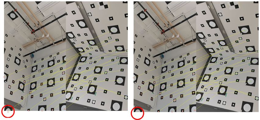
The Photogrammetric Record

        (1) an efficient procedure to define exact point correspondences between images; and
        (2) an appropriate geometric camera model to describe the IOPs.
     To find exact point correspondences, centres of circular targets, such as those shown in
the calibration laboratory of Fig. 1, are almost exclusively utilised in high-precision close-
range photogrammetry applications (Luhmann, 2014). Circular targets are geometrically
approximated by ellipses in images. They offer several advantages such as a unique centre,
invariance under rotation and translation, and low cost of production. As the number of
targets, as well as images, increases, on the one hand the manual matching of corresponding
targets becomes more tedious, time consuming and impractical. On the other hand,
automated matching using only the geometric characteristics of ellipses, runs the risk of
mismatches (type II errors, also termed false negatives or omission errors). Therefore, coded
targets were recommended to reduce the effects of type II errors during target matching
(Shortis and Seager, 2014). Coded targets, however, still require the design of a distinct
unique identifier as well as manual labelling of targets individually, which may serve to be
impractical in large target fields. A fully automated process to identify and match targets
with minimal manual intervention is, hence, desirable for larger target fields with larger
number of images.
     In addition, even though the circular targets in object space are projected as ellipses in
the image plane, the centres of the best-fitting ellipses in the images do not necessarily
correspond to the actual centre of the circular target. This is commonly referred to as the
eccentricity error, which is a consequence of the projective geometry. The systematic
eccentricity error suggests that for two corresponding ellipses in two or more image views,
the 3D reconstructed centres of the best-fitting ellipses, even in the absence of random or
systematic errors, will not correspond to the centre of the original circular targets (Luhmann,
2014). Hence, the systematic eccentricity error in images must be corrected, especially in
applications requiring high-precision metrology.
     The other important consideration for camera calibration is the selection of the appropriate
geometric camera model. Especially for new optical instruments, such as newly released
smartphone cameras, the extent of the impact of the additional parameters, including the terms
required to correct radial lens distortions, must be evaluated. In this study the goal is to model
the IOPs and the requirements for metric calibration of 4K video recordings, acquired using

         (a)                         (b)                       (c)                        (d)                  (e)

FIG. 1. Process to collect video data for calibration: (a) corner of the calibration laboratory; (b) bottom of the
ladder facing the ceiling in portrait; (c) top of the ladder facing the floor in portrait; (d) top of the ladder facing
               the floor in landscape; and (e) bottom of the ladder facing the ceiling in landscape.

© 2021 The Authors
The Photogrammetric Record published by Remote Sensing and Photogrammetry Society and John Wiley & Sons Ltd.           125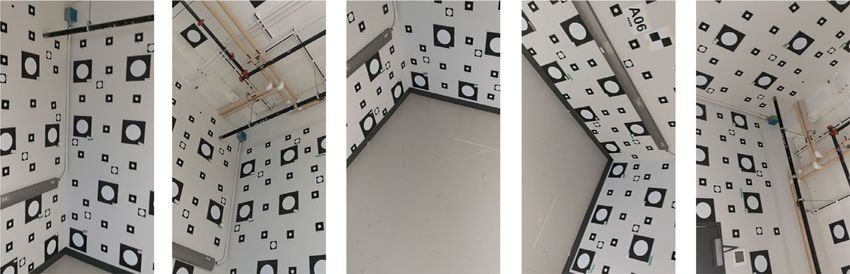
MAALEK and LICHTI. Automated calibration of smartphone cameras for 3D reconstruction of mechanical pipes

three of the latest smartphone cameras, namely, the iPhone 11, the Huawei P30 and the Samsung
S10. Video recordings were utilised since the broader application of this study pertains to
progress monitoring of mechanical pipes on construction projects, which is more practical using
video recording (as opposed to single images). The real-world impact of the calibration
parameters on estimating the geometric parameters of cylinders representing mechanical pipes,
in support of as-built documentation of construction sites, will also be examined.
     To this end, this study focuses on:

  (i) developing an automated and robust method to detect and match circular targets
      between video images;
 (ii) providing a simple approach to correct the eccentricity error;
(iii) identifying the geometric error modelling requirements of the mentioned smartphone
      cameras; and
(iv) determining the extent of the impact of the camera geometric modelling on the
      accuracy of a 3D reconstructed mechanical pipe.

                                             Literature Review
     The review of previous literature has been divided into two main categories:
(i) matching conics between images; and (ii) geometric models for the calibration of
smartphone cameras. These two are further explained in the following sections.

Matching Conics between Images
    Given the camera matrices of two views, P and P0, the necessary and sufficient
conditions for matching conics is given by Δ as follows (Quan, 1996):
                      8
                      >
                      > devðVÞ ¼ detðA þ λBÞ ¼ I 1 λ4 þ I 2 λ3 þ I 3 λ2 þ I 4 λ þ I 5
                      >
                      < A ¼ PT CP
                                                                                                                          (1)
                      >
                      > B ¼ P0T C0 P0
                      >
                      :
                         Δ ¼ I 23  4I 2 I 4 ¼ 0

where C and C0 are the conic’s algebraic matrices corresponding to views P and P0 ; V is
the characteristic polynomial of matrices A and B; I j : j ¼ 1⋯5 are the coefficients of the
determinant of V, detðVÞ; and ð:ÞT denotes a matrix transpose. Equation (1) shows that, for
two matching conics between two views, Δ is equal to zero (or very close to zero in the
presence of measurement errors). The problem of automated matching of conics between
two images, hence, requires the automated: (i) detection of conics; and (ii) determination of
camera matrices. A comprehensive discussion of available and novel methods for detecting
non-overlapping ellipses from images was given in Maalek and Lichti (2021b). The
remainder of this section, therefore, focuses on the latter requirement, namely automated
methods of recovering camera matrices, given only point correspondences.

     Recovering Camera Matrices. Fundamental matrices are widely implemented in
computer vision to provide an algebraic representation of epipolar geometry between two
images. Given a sufficient set of matching points (at least seven), the fundamental matrix
(F) can be estimated (Hartley and Zisserman, 2004). An important property of fundamental
matrices is that the estimated F between two views is invariant to projective transformation

                                                                                                            © 2021 The Authors
126                The Photogrammetric Record published by Remote Sensing and Photogrammetry Society and John Wiley & Sons Ltd.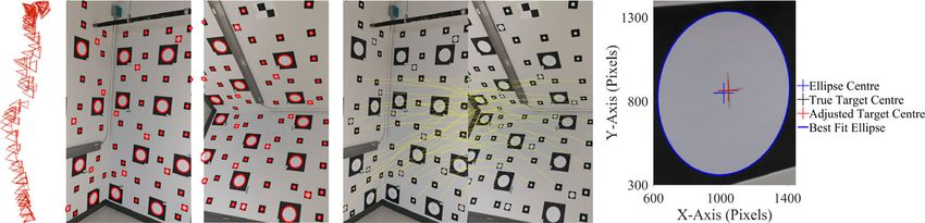
The Photogrammetric Record

of the object space. Therefore, the relative camera matrices can be obtained directly by the
fundamental matrix up to a projective ambiguity (Luong and Viéville, 1996). If the camera
model is assumed unchanged between two views, the reconstruction is possible up to an
affine ambiguity. In case an initial estimate of the IOPs is available, the fundamental matrix
can be decomposed into the essential matrix, E ¼ KT FK, where K represents the matrix of
intrinsic camera parameters (IOPs). Given matrix K, the relative orientation between two
cameras can be retrieved through singular-value decomposition of the essential matrix
(Hartley and Zisserman, 2004) with only five point correspondences (Stewénius et al.,
2006). In such cases, it is possible to recover the reconstruction up to a similarity
transformation (an arbitrary scale factor). The two-view process can also be extended to
multiple image views. In fact, the camera matrices of m images can be recovered, given at
least m  1 pairwise fundamental matrices and epipoles, using the projective factorisation
method of Sturm and Triggs (1996). The latter is an example of a global reconstruction
framework. In practice, however, a sequential reconstruction and registration of new images
typically produces more reliable results, due to the flexibilities and control inherent in the
incremental improvement of the reconstruction solution (Schönberger, 2018).

      Sequential Structure from Motion (SfM). Structure from motion is the process of
retrieving camera IOPs and EOPs subject to rigid-body motion (namely rotation and
translation (Ullman, 1979)). An overview of a typical sequential SfM comprises the
following steps:

(1) Detect and match features between every pair of images and determine overlapping
    images. The point correspondences are typically obtained automatically using
    established computer vision feature extraction and matching methods such as the scale-
    invariant feature transform (SIFT: Lowe, 2004), speeded-up robust features (SURF: Bay
    et al., 2008), or their variants.
(2) Start with an initial pair of images (typically the two images obtaining the highest score
    for some geometric selection criterion; see Schönberger (2018).
(3) Estimate the relative orientation and camera matrices between the two images using
    corresponding feature points. Note that an initial estimate of the IOPs is typically
    required for this stage.
(4) Triangulate to determine 3D coordinates of the corresponding points.
(5) Perform a bundle adjustment to refine IOPs and EOPs.
(6) For the remaining images, perform the following:
      (a) Add a new overlapping image to the set of previous images.
      (b) Estimate the relative orientation parameters of the new image from the existing
          overlapping feature points.
      (c) Using step 1, determine the new matching feature points and triangulate them to
          estimate the object-space coordinates of the new feature points.
      (d) Perform a bundle adjustment to refine the IOPs and EOPs.
      (e) Perform steps 6(a) through (d) until all images are examined.
     The output of SfM is a set of EOPs, IOPs and image feature points, as well as sparse
object-space point clouds. Several approaches, as well as software packages, exist that
perform different variants of SfM. In this study, COLMAP, an open-source software
package comprised of many computational and scientific improvements to traditional SfM
methods, as documented in Schönberger (2018), was utilised.

© 2021 The Authors
The Photogrammetric Record published by Remote Sensing and Photogrammetry Society and John Wiley & Sons Ltd.           127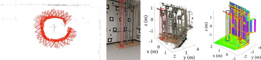
MAALEK and LICHTI. Automated calibration of smartphone cameras for 3D reconstruction of mechanical pipes

Geometric Models for Smartphone Camera Calibration
       Smartphone cameras can be considered as pinhole cameras for which the collinearity
condition can be used to model the straight-line relationship between an observed image
point (x, y), its homologous object point (X , Y , Z) and the perspective centre of the camera
(X c , Y c , Z c ), as described in Luhmann et al. (2014). Random error departures from the
hypothesised collinearity condition are modelled as additive, zero-mean noise terms (ɛ x , ɛ y )
while (Δx, Δy) represent systematic error correction terms. The latter comprise the models
for radial lens distortion and decentring distortion. Radial lens distortion, which is by far the
larger of the two distortions, is most often modelled with three terms of the standard
polynomial (such as Luhmann et al., 2016), though higher-order terms have been
demonstrated to be required for wide-angle lenses (Lichti et al., 2020). Images collected
with modern smartphone cameras are generally corrected for radial lens distortion. However,
the extent of the correction and the metric impact, if any, on object-space reconstruction is
not known and a subject of this investigation.

                                                 Methodology
     The proposed method for metric calibration of smartphone cameras is formulated as
follows:

(1) Calibration data collection: which involves the method for data collection from the
    calibration laboratory (Fig. 1).
(2) Circular target centre matching: which consists of the following stages:
      (a)   Estimation of camera projective matrices (Fig. 2(a)).
      (b)   Automated ellipse detection from images (Fig. 2(b)).
      (c)   Automated ellipse matching between images (Fig. 2(c)).
      (d)   Correction of ellipse eccentricity error (Fig. 2(d)).
(3) Self-calibrating bundle adjustment.
      Each section is introduced in more detail in the following sections.

Calibration Data Collection
       This study focuses on the calibration of smartphone cameras using video sequences. To
improve the precision of the self-calibration and prevent projective compensation (coupling),
the recordings must: (i) capture depth variation in the target field; (ii) be convergent; and
(iii) rotate 90° about the camera’s optical axis (thus both landscape and portrait images). One
corner of a complete calibration laboratory was utilised (Fig. 1(a)), which consists of multiple
targets attached to two right-angled intersecting walls. The two intersecting planar walls were
utilised to create depth variation in the target field. A ladder was used to collect convergent
images of the scene, starting from the bottom of the ladder facing the ceiling (Fig. 1(b)) and
ending at the top of the ladder facing the floor (Fig. 1(c)). At the top, the camera was rotated
90° and the video was then recorded in the reverse order (Figs. 1(d) and (e)).

Circular Target Centre Matching
    The problem of circular target matching for calibration requires: (i) estimation of
camera projective matrices (Fig. 2(a)); (ii) automated detection of ellipses from each image

                                                                                                            © 2021 The Authors
128                The Photogrammetric Record published by Remote Sensing and Photogrammetry Society and John Wiley & Sons Ltd.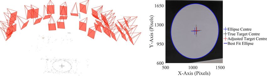
The Photogrammetric Record
(a) (b) (c) (d)
FIG. 2. Output of the proposed steps to acquire matching target centres between images: (a) estimated camera
position and orientation (EOPs) using Algorithm 1; (b) detected ellipses using the method of Maalek and Lichti
(2021a) for two images; (c) automatic matching of corresponding target centres using Algorithm 2; and
(d) correction of the estimated target centre in image plane using Algorithm 3.
(Fig. 2(b)); (iii) correct matching of corresponding ellipses between different images
(Fig. 2(c)); and (iv) correction of the eccentricity error of the ellipses’ centres (Fig. 2(d)).
These steps are discussed in more detail below.
Estimating the Camera Projective Matrices. Based on the discussions above, an initial
estimate of the camera projective matrices (comprised of IOPs and EOPs) can be obtained
using an SfM framework, such as COLMAP. Here, Algorithm 1 is proposed to further
improve the estimated camera matrices, retrieved from the outputs of COLMAP’s sparse
reconstruction:
A 1: Refining Camera Matrices
(1) Determine the features used for sparse reconstruction in images from COLMAP.
(2) Between every two images with overlapping features, and
, where is the total number of images, perform the robust least
median of squares (LMedS; (Rousseeuwand Leroy, 1987)) fundamental matrix
estimation, using the subsample bucketing strategy of Zhang (1998), to retrieve
the inlier features and fundamental matrix.
(3) For the inlier matching feature points ofstep 2, perform the robust triangulation
using LMedS with random subsampling. Identify the inlier feature points for
every given sparsely reconstructed point.
(4) Perform the bundle adjustment only on the inlier features of steps 2 and 3 (thus
weighting all outlying features as zero) to retrieve the refined EOPs and IOPs.
As a point of reference, Fig. 2(a) illustrates the estimated camera positions and
orientations of a sequence of images collected with the proposed strategy using Algorithm
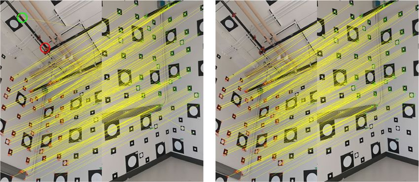
1. Fig. 3 shows the refinement of the matched features using Algorithm 1. As observed, two
mismatched features, represented by red and green circles, were correctly removed. The red
circle indicates a feature point that did not satisfy step 2 of Algorithm 1, whereas the
© 2021 The Authors
The Photogrammetric Record published by Remote Sensing and Photogrammetry Society and John Wiley & Sons Ltd. 129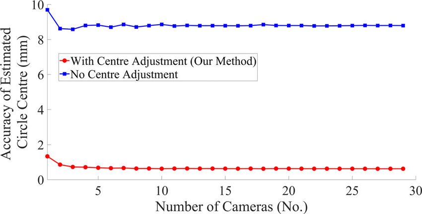
MAALEK and LICHTI. Automated calibration of smartphone cameras for 3D reconstruction of mechanical pipes

 (a)                                                            (b)

FIG. 3. Matched features between images. (a) Results from COLMAP. (b) Results of refinements using
Algorithm 1. Note that the two mismatched features, represented by red and green circles in (a), were correctly
                                              removed in (b).

mismatched feature indicated by the green circle was removed using step 3. In this example,
even though the refinement is marginal, two mismatches out of around 300 correct matches
can still negatively affect the results of the estimated IOPs and EOPs, especially when most
images contain mismatches.

     Automated Ellipse Detection from Images. The robust ellipse detection method
presented in Maalek and Lichti (2021b) is used to detect non-overlapping ellipses of the
projected circular targets. The method was shown to provide ellipse detection with superior
robustness to both type I errors (false positives; commission errors) and type II errors (false
negatives; omission errors), compared to the established ellipse detection methods of
Fornaciari et al. (2014) and Pǎtrǎucean et al. (2017). Once the ellipses are detected, the
best-fitting geometric parameter vector of each ellipse is estimated using the new confocal
hyperbola ellipse fitting method, presented in Maalek and Lichti (2021a). The geometric
parameters of the ellipse (centre, semi-major length, semi-minor length and rotation angle)
are then converted to algebraic form, which are then transformed into matrix form to be
used for conic matching through equation (1).

     Automated Ellipse Matching between Images. Equation (1) is utilised here to verify
possible matching conics between two images. A brute-force matching strategy suggests
checking the correspondence condition, Δ of equation (1), for every detected ellipse of an
image to all ellipses of all other images, which can become computationally expensive with
a larger number of images with many targets. In addition, Δ calculated using equation (1) is
not necessarily equal to zero in the presence of systematic and random measurement errors
(Quan, 1996). Therefore, a threshold is required on jΔj to model the matching uncertainties
in the presence of measurement errors. An arbitrarily selected threshold for the
correspondence condition Δ will, however, almost guarantee either mismatches (type II
errors) or no matches (type I errors).
     Here, instead of comparing all conics together in a brute-force fashion, first, only a
select set of candidates are considered, whose centres in both images satisfy an adaptive

                                                                                                             © 2021 The Authors
130                 The Photogrammetric Record published by Remote Sensing and Photogrammetry Society and John Wiley & Sons Ltd.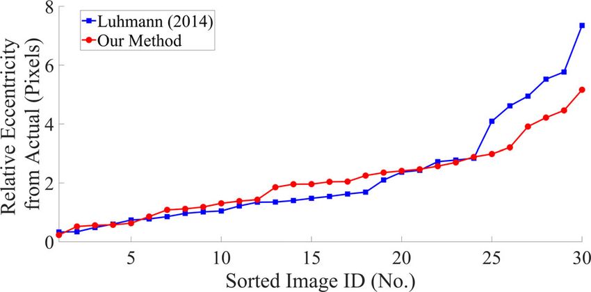
The Photogrammetric Record

closeness constraint on the corresponding epipolar distance. Amongst the available ellipses
satisfying the epipolar constraint, that achieving the smallest jΔj is chosen as the matching
conic. This process is attractive for two reasons. First, since the robust fundamental matrix
between two images is already computed automatically using the LMedS method in
Algorithm 1 (step 2), the agreement of the inlier points to the estimated fundamental matrix
can be used as a basis to compute the threshold for the epipolar constraint on the centres as
well (no predefined subjective threshold is required). Second, the ellipse matching using the
correspondence condition of equation (1) requires no threshold. To formulate the proposed
process, Algorithm 2 is provided as follows:
     Step 4(b) of Algorithm 2 performs the pairwise conic matching condition on only a
selected set of inlier ellipse centres that lie near the epipolar line. Furthermore, instead of
choosing an arbitrary threshold for Δ, the minimum of jΔj is used. To further reduce the effects
of type II errors (mismatching targets), the robust triangulation using LMedS is performed.

      Correction of Ellipse Eccentricity Error. Modelling the eccentricity error for circular
targets has been the subject of investigation, especially in high-precision metrology (Ahn
et al., 1999; He et al., 2013; Luhmann, 2014). Closed formulations of the eccentricity error
in both the image plane and object space exist (Dold, 1996; Ahn et al., 1999). The available
correction formulations for the errors in the image plane, however, require the knowledge of
the target’s object-space parameters, such as the radius of the target, the object-space
coordinates of the centre and the normal vector of the circular target’s plane. This
information, however, cannot be trivially retrieved. Even if a reliable external measurement
of the object space exists, the additional constraint will be undesirable in free-network self-
calibration practices, which is the focus of this study. In the following, a process is
presented to retrieve the projection of the true centre of the circular target onto the image,
given only the matching target parameters in two views.
      Following the formulation of equation (1), Quan (1996) proposed a process to acquire
the equation of the object-space plane where the conic lies, given two camera projection
matrices and the conics’ algebraic matrices in the image plane. The subsequent object-space
conic’s equation for the matching conics can then be retrieved by intersecting the plane with
the cone’s equation (see equation (1)). Ideally, the object-space conic should be represented
by a circle in the case of circular targets, however, due to measurement errors and
uncertainties in the estimation of the projection matrices, the object-space conic might be an
ellipse. The object-space centre of the ellipse (or circle) can be directly extracted from the
retrieved conic’s equation. The corrected centre in the image can, hence, be extracted by
back projecting the object-space centre of the retrieved ellipse onto the image planes. Since
multiple views of a given target may be imaged, the final consideration is to determine the
best view for a particular target. To this end, two criteria are used: (i) the convergence angle
between the two views; and (ii) the uncertainty of the object-space centre estimation. First,
for a given view, only the image views with an average convergence angle of more than
20° (Schönberger, 2018) are considered. Second, for a specific matched target, the
uncertainty of the object-space centre estimation is characterised, here, as the covariance of
the 3D reconstructed ellipse centres between a given view and another acceptable view. The
covariance is estimated using the formulation provided by Beder and Steffen (2006). The
two views achieving the minimum determinant of the covariance matrix (MCD) –
representing the pair with the minimum uncertainty – are selected as the ideal candidate
(Rousseeuw and Leroy, 1987). Intuitively, the latter selection criterion provides the pair of
images whose object-space coordinates in the vicinity of the true centre are the least

© 2021 The Authors
The Photogrammetric Record published by Remote Sensing and Photogrammetry Society and John Wiley & Sons Ltd.           131
MAALEK and LICHTI. Automated calibration of smartphone cameras for 3D reconstruction of mechanical pipes
A 2: Automated Matching of Ellipses
(1) Estimate the camera projective matrices using Algorithm 1.
(2) Detect the ellipses using the robust non-overlapping ellipse detection of Maalek
and Lichti (2021a).
(3) For each detected ellipse, find the best-fitting ellipse using the method of Maalek
and Lichti (2021b) and construct the equivalent algebraic conic matrix.
(4) For every pair of overlapping images, and ,
where is the total number of images, find the matching ellipses as follows:
(a) From the LMedS algorithm of step 1:
(i) Use the solutions obtained for the fundamental matrix, .
(ii) Calculate the standard deviation of the epipolar distance (Hartley and
Zisserman, 2004), , of the inlier matches.
(b) For each ellipse centre in image , , find the ellipse centres in image ,
, that satisfies the following condition:
χ
(2)
where is the epipolar distance between image points ,
and χ is the chi-squared cumulative probability distribution function
with probability 97.5% and 2 degrees of freedom for 2D data.
(c) For all ellipse candidates satisfying equation (2) between two images,
perform the following:
(i) Select all related matching ellipses between the two images. For
instance, if ellipse labels 5 and 6 of image satisfy equation (2) for
the ellipse labelled 4 of image , all other ellipses of image that
satisfy equation (2) for ellipses labelled 5 and 6 of image should also
be selected, and so on.
(ii) Calculate ∆ from equation (1) between the ellipse candidates (from
the previous step) of images and .
(iii) Two ellipses are considered to be matching if and only if both ellipses
achieved the minimum |∆| for each other. For instance, if the ellipse
labelled 5 of image achieved the smallest |∆| for label 4 of image ,
the two will only be matched if the ellipse labelled 4 of image
achieves the smallest |∆| for label 5 of image .
(5) Using the matched ellipses of step 4 in two views (image pairs), determine the
matching ellipse between all other images.
(6) Using the multiview correspondences identified in step 5, for each ellipse
perform the following steps to reduce the impact of type II errors (mismatches):
(a) Use the camera projective matrices estimated in step 1.
(b) Perform a robust multiview triangulation on the ellipse centres using
LMedS (or any other preferred robust method).
(c) Retain only the inlier set of corresponding ellipse centres.
(7) The inlier ellipse correspondences are the final set of matched ellipses.
© 2021 The Authors
132 The Photogrammetric Record published by Remote Sensing and Photogrammetry Society and John Wiley & Sons Ltd.The Photogrammetric Record
uncertain. The process is formulated using Algorithm 3 for each identified target with two
or more image view correspondences, as follows:
The results of Algorithm 3 are fed to a free-network self-calibrating bundle adjustment
that estimates the EOPs, IOPs and object-space coordinates of the targets. Once the EOPs
and IOPs are determined, the centres can again be adjusted and recursively fed into the
bundle adjustment to refine the results up to the required/satisfactory precision. Furthermore,
Algorithm 3 can be utilised before the robust triangulation step of Algorithm 2 (after step 4)
so that possible correct matches are not incorrectly rejected (improving type I errors in
target matching). Fig. 4 illustrates the results of using Algorithm 3 within Algorithm 2. In
this example, one additional target was correctly matched (amongst a total of 23
overlapping targets) when applying Algorithm 3 within Algorithm 2.
Self-calibrating Bundle Adjustment
The final step of the algorithm is the self-calibrating bundle adjustment, which is the
accepted standard methodology for obtaining the highest accuracy (Luhmann et al., 2016).
Provided that the aforementioned design measures have been incorporated into the imaging
network, the IOPs will be successfully decorrelated from the EOPs and, thus, recovered
accurately. Any outlier observations have been successfully removed by this stage of the
algorithm, so a least-squares solution can be utilised for the parameter estimation. The IOPs
(which are considered network-invariant – one set per camera), EOPs and object points are
estimated. The singularity of the least-squares normal-equations matrix caused by the datum
defect is removed by adding the inner constraints (free-network adjustment (Luhmann et al.,
2014)) since this yields optimal object point precision.
Following the self-calibration adjustment, the solution quality can be examined with
several computed quantities. Most important among these are the estimated IOPs and their
precision estimates, together with derived correlation coefficient matrices that quantify the
success of the parameter decorrelation. The residuals are crucial for graphically and
statistically assessing the effectiveness of the lens distortion modelling. The presence of
unmodelled radial lens distortion, for example, can be readily identified in a plot of the
radial component of the image point residuals as a function of radial distance from the
principal point. Moreover, reconstruction accuracy in object space can be quantified by
comparing the photogrammetrically determined coordinates of (or derived distances
between) targets with reference values from an independent measurement source.
Summary of Methods
The proposed camera calibration framework can be summarised as follows:
(1) Determine an initial estimate of the EOPs and IOPs using available SfM methods
or software packages (here, COLMAP was used).
(2) Refine the estimated EOPs and IOPs to calculate the modified camera projective
matrices for each image view using Algorithm 1.
(3) Determine the ellipses in each image using the robust non-overlapping ellipse
detection of Maalek and Lichti (2021b).
(4) Match overlapping ellipses between all views using Algorithm 2.
(5) Adjust the eccentricity error of the estimated ellipse centres of all matched
ellipses using Algorithm 3.
© 2021 The Authors
The Photogrammetric Record published by Remote Sensing and Photogrammetry Society and John Wiley & Sons Ltd. 133MAALEK and LICHTI. Automated calibration of smartphone cameras for 3D reconstruction of mechanical pipes
A 3: Correcting Eccentricity Error
(1) Retain the object-space coordinate of the target’s centre from Algorithm 2.
(2) Identify all images corresponding to the considered target, say images ,
where is the number of views corresponding to a given target.
(3) For each image , find the best image pair in , (image
pair with the least uncertainty in the estimated target’s centre) as follows:
(a) Find all images in whose average convergence angle from
image is more than 20° (Schönberger, 2018).
(b) Estimate the covariance matrix of the 3D reconstructed ellipse centres of
the views obtained by the previous step using Beder and Steffen (2006).
(c) For image , find the corresponding pair whose determinant of the
covariance matrix is minimum (MCD).
(d) Repeat the steps 3(a) to 3(c) to find a best image pair for all images .
(4) For image with the selected best image }, perform the
following steps to retrieve the corrected ellipse centre in image :
(a) Determine the object space plane parameters, =( ) , of the
conic in space using the method of Quan (1996).
(b) Intersect plane with the cone (for image ) to find the conic equation
as follows ( explained in equation (1)):
(i) Parametrically derive the coordinate as a function of and using
the planes’ equation as follows:
(3)
(ii) Substitute into the cone’s equation to derive the object-space conic
matrix of the ellipse, , as follows:
1 (4)
1 1
(iii) Calculate the geometric centre ) of the ellipse corresponding to
the conic matrix as follows:
= =− (5)
where is the 2×2 matrix constructed after removing row and
column from .
(iv) Substitute ) into equation (3) to calculate the component of
the object-space 3D coordinates of the centre of the ellipse
= ).
(v) Project the centre of the conic back onto the image plane to find the
corrected centre, , where is the camera projective
matrix for image .
(vi) Convert the estimated centres into homogeneous coordinates for use
in the bundle adjustment.
(5) Once the target’s centre in all images has been corrected, perform triangulation
to correct the object-space coordinates of the centre.
© 2021 The Authors
134 The Photogrammetric Record published by Remote Sensing and Photogrammetry Society and John Wiley & Sons Ltd.The Photogrammetric Record
(a) (b)
FIG. 4. Impact of centre correction on the results of the target matching between two sample images: (a) without
centre correction; and (b) with centre correction.
(6) Perform the proposed free-network self-calibrating bundle adjustment to estimate
the EOPs and IOPs.
(7) Perform steps 4 through 6 with the new EOPs and IOPs until the sets of matched
ellipses between two consecutive iterations remain unchanged.
The final set of IOPs is the solution to the calibration.
Selection of Terms for Radial Lens Distortion
The accuracy of 3D reconstruction from a camera system affected by lens distortions
can be significantly impacted by the choice of systematic error correction terms included in
the augmented collinearity condition. The aim is to find a trade-off between goodness-of-fit
and allowable bias. One must avoid an underparameterised model with an insufficient
number of terms to describe the distortion profile that can lead to the propagation of bias
into other model parameters and optimistic parameter precision. On the other hand,
overparameterisation by adding more terms than necessary can introduce correlations among
model variables that can inflate the condition number of the normal-equations matrix and, in
turn, degrade reconstruction accuracy. To this end, a process similar to that described in
Lichti et al. (2020) was employed. Using the final set of matched targets, an initial self-
calibration solution was performed without any lens distortion parameters. The interior
geometry of the camera in this adjustment was described only by the principal point and
principal distance. Graphical analyses of the estimated residuals, supported with statistical
testing and information criteria, were utilised to make an informed decision about the
coefficients to be added. In particular, the radial component of the image point residuals, vr ,
plotted as a function of radial distance from the principal point, r, was graphically assessed.
A single parameter was then added to the model and the self-calibration was recomputed.
The process was repeated until no systematic trends remain.
© 2021 The Authors
The Photogrammetric Record published by Remote Sensing and Photogrammetry Society and John Wiley & Sons Ltd. 135MAALEK and LICHTI. Automated calibration of smartphone cameras for 3D reconstruction of mechanical pipes
Resulting Smartphone Calibration Parameters and Conditions
A total of 1.5 minutes of 4K videos at 30 frames per second (fps) was recorded as per
the presented data collection method above using the Huawei P30, iPhone 11 and Samsung
S10 smartphones. The portion of the calibration laboratory used in this study contained 130
targets. The recorded videos using each smartphone instrument were captured so as to fill
the frame with the same 130 targets for consistency. The Open Camera app was utilised,
where possible, to help access raw smartphone camera configurations, such as adjusting the
focus to infinity, disabling autofocus and fixing the camera exposures. From the 1.5 minutes
of video footage, 90 image frames at 1 fps were decomposed: these were used within the
proposed frameworks of Algorithms 1 to 3 to calibrate the smartphone cameras. The
convergence angles were 80°, 88° and 109° for the P30, iPhone 11 and S10 networks,
respectively. The final set of IOPs, including the selected terms for correction of radial lens
distortion, are shown in Table I.
Method of Validation of Results
The effectiveness of Algorithm 2 requires the quantification of the quality of ellipse
matching between different images. Here, the four main metrics commonly used to
determine the quality of object-extraction algorithms (precision, recall, accuracy and F-
measure: Olson and Delen, 2008), were utilised:
8
> TP
>
> Precision ¼
>
> T P þ FP
>
>
>
>
>
> TP
>
< Recall ¼
T P þ FN (6)
>
> þ
>
> T P T N
>
> Accuracy ¼
>
> T P þ T N þ FP þ FN
>
>
>
: F measure ¼ 2 Precision Recall
>
Precision þ Recall
where T P , T N , F P , F N are the number of true positives, true negatives, false positives and
false negatives of the object-extraction algorithm, respectively. To measure the accuracy of
estimated parameters, such as centre adjustment in Algorithm 3, the Euclidian distance (or
L2 norm) of the estimated parameters from the final ground-truth parameters were used. The
ground truth in each experiment was determined manually.
Table I. Summary of the estimated IOPs for each smartphone using the proposed methodology.
Device Principal Principal Radial distortion parameters
point (px) distance (px)
k1 k2 k3 k4 k5
Huawei P30 (1086.7, 1915.2) 3762.3 1.9E−08 −2.1E−14 1.1E−20 −2.5E−27 2.0E−34
σ
á
(0.2, 0.3) 0.9 4.6E−10 5.7E−16 3.1E−22 7.4E−29 6.5E−36
iPhone 11 (1087.9, 1896.3) 3411.4 8.9E−09 −1.4E−15 4.4E−23 0 0
σ – –
á
(0.1, 0.1) 0.6 5.3E−11 2.6E−17 3.9E−25
Samsung S10 (1136.5, 1953.8) 3002.6 2.0E−08 −7.5E−15 9.8E−22 −1.4E−25 0
σ –
á
(0.8, 0.8) 1.5 5.0E−10 2.5E−17 3.9E−24 6.1E−27
© 2021 The Authors
136 The Photogrammetric Record published by Remote Sensing and Photogrammetry Society and John Wiley & Sons Ltd.The Photogrammetric Record
(a) (b)
FIG. 5. Design of the evaluation of ellipse eccentricity adjustment experiment: (a) EOPs for the 28 image views;
(b) ellipse centre, adjusted target centre and true target centre for a sample image and target.
Experiment Design
Four experiments were designed to assess the effectiveness of the proposed methods
used in this study, namely: evaluation of ellipse eccentricity adjustment, incorporating two
experiments (impact of centre adjustment and comparison of eccentricity error); quality
assessment of ellipse matching; and evaluation of impact of calibration on pipe
reconstruction. The four experiments are explained in more detail in the following.
Evaluation of Ellipse Eccentricity Adjustment
Algorithm 3 was developed to correct the eccentricity error of the estimated centre of
the targets in images due to projective transformation. This experiment is designed to
evaluate the effectiveness of the proposed method in practical settings. To this end, 28
image frames were taken from 4K video recording of a single target using a pre-calibrated
Huawei P30. The EOPs of each image view were estimated using COLMAP and shown in
Fig. 5(a). The ground-truth target centre in each image was manually determined from the
pronounced black cross (Fig. 5(b)). The radius of the circular target was 100 mm and the
images were taken from an average of 530 mm from the circular target. The scale of the 3D
reconstruction was manually defined using the radius of the circular target. The precision of
the 3D reconstructed centre using the ground-truth image centres and estimated EOPs was
0.13 mm. The ground-truth centre, the estimated best-fitting ellipse centre and the adjusted
centre using Algorithm 3 for one sample image are shown in Fig. 5(b)). Two experiments
were designed to: (i) quantify the impact of centre adjustment on the accuracy of the 3D
reconstructed centre; and (ii) evaluate its performance compared to the closed formulation of
eccentricity error by Luhmann (2014).
Impact of Centre Adjustment on the 3D Reconstruction. In this experiment, the impact
of adjusting the eccentricity error compared to the estimated best-fitting ellipse centre
(unadjusted) on the accuracy of the 3D reconstructed centre of the target was evaluated as
the number of camera views increased from 2 to 28. Since different combinations of views
will generate different reconstruction results, for a given number of (say k) image views, N
different combinations of k = 2. . .28 images were selected. To this end, for k image views,
the following steps were carried out:
© 2021 The Authors
The Photogrammetric Record published by Remote Sensing and Photogrammetry Society and John Wiley & Sons Ltd. 137MAALEK and LICHTI. Automated calibration of smartphone cameras for 3D reconstruction of mechanical pipes
(1) Randomly select N different combinations of k images from the 28 images.
(2) For each set of k images, using the estimated best-fitting ellipse centre (no
adjustment), adjusted centre using Algorithm 3 and camera projection matrices
(Fig. 5(a)), perform triangulation (Hartley and Zisserman, 2004) and determine the
object-space position of the target centres.
(3) Calculate the Euclidian distance between the object-space coordinates of the
adjusted and unadjusted centres (separately) from the ground-truth centre.
(4) For the given number of image views, k, record the mean of the N distances
obtained from step 3 for the adjusted and unadjusted centres.
Here, N = 50 combinations were selected.
Comparison of Eccentricity Error between Algorithm 3 and Luhmann’s Formula. A
closed formulation of the centre eccentricity error in the image plane was provided in
Luhmann (2014), given the EOPs and IOPs of the view, 3D object-space target centre,
object-space target radius and target plane’s normal. To determine the eccentricity error
using Luhmann’s formula, the ground-truth 3D object-space centre, the radius, as well as
the plane normal, were used. For each image, the eccentricity errors (in pixels) were
calculated using both the authors’ method (Algorithm 3) and Luhmann’s formula. For each
image, both eccentricity errors in each image were then compared to the ground-truth
eccentricity error and reported.
Quality Assessment of Ellipse Matching
This experiment was designed to assess the quality of the ellipse matching results,
obtained by Algorithm 2. The 270 images from the calibration laboratory, reported above in
the section Resulting Smartphone Calibration Parameters and Conditions, were used. The
ellipses of the 270 images were extracted using the method of Maalek and Lichti (2021b).
The camera projective matrices as well as the detected ellipses for each image were then fed
to Algorithm 2 to determine the matching ellipses between different images. The quality of
matching was quantified for three settings: Algorithm 2 without robust triangulation;
Algorithm 2 with robust triangulation; and Algorithm 2 with robust triangulation and
corrected centres.
Evaluation of Impact of Calibration on Pipe Reconstruction
The broader objective of this study pertains to the application of smartphone cameras
for 3D reconstruction of pipes. To this end, mechanical mock pipes were professionally
installed at one corner of the calibration laboratory, shown in Fig. 6. This experiment was
designed to assess the effectiveness of the proposed calibration process in estimating the
radius of the pipe of interest after 3D reconstruction. Here, the accuracy of the estimated
radius using the authors’ pre-calibration process and lens distortion modelling was compared
with that obtained using COLMAP’s default SfM process. The latter involves an in situ
automatic calibration, comprised of the first two terms of the radial lens distortion
parameters, using the exchangeable image file (Exif) data as the initial IOP estimation. This
latter process, from here on, is referred to as COLMAP-radial.
A 60-second 4K video was recorded around one pipe using each of the Huawei
P30, iPhone 11 and Samsung S10 smartphones. The recording was divided into two
30-second videos (at 1 fps), one in portrait mode and the other in landscape mode. The
© 2021 The Authors
138 The Photogrammetric Record published by Remote Sensing and Photogrammetry Society and John Wiley & Sons Ltd.The Photogrammetric Record
(b) (c) (d)
(a)
FIG. 6. Design of the “evaluation of impact of calibration on pipe reconstruction” experiment: (a) sample path
around the pipe investigated; (b) sample image of the pipe with the targets on the background wall. 3D point
cloud of the mock pipes using: (c) SfM 3D reconstruction; and (d) HDS6100 TLS.
camera was rotated 90° about its optical axis at a different height so as to provide
COLMAP-radial a reasonable opportunity to calibrate the instruments without possible
projective coupling. A dense 3D reconstruction was then carried out using COLMAP,
once with the IOPs obtained by COLMAP-radial and then again with the authors’ target-
based calibration framework.
The final consideration for the 3D reconstruction was to define the scale. Since the
accuracy of estimating the radius of the cylinder is being considered, it is important to
define the scale of the 3D reconstruction independently from the cylinder’s radius. The scale
of the reconstruction is, hence, defined using the distance of two of the targets behind the
mock pipes (Fig. 6(b)). The ground-truth distance between the targets was determined using
a Leica Geosystems HDS6100 terrestrial laser scanner (TLS). The following process was
then performed to determine the scale:
(1) Detect the ellipses in images using the ellipse detection method of Maalek and
Lichti (2021b).
(2) Match the detected ellipses between images using Algorithm 2.
(3) Select two of the targets with the maximum number of image views.
(4) Adjust the centre eccentricity error of the two targets in each image view using
Algorithm 3.
(5) Triangulate to determine the 3D coordinates of the two targets.
(6) Determine the ground-truth 3D coordinates of the centre of the two targets in the
TLS point cloud using the method presented in Lichti et al. (2019b).
(7) The scale is defined by the ratio between the ground-truth distance (step 6) and
the 3D reconstructed distance (step 5) of the two targets.
The radius of the cylinder of interest for the scaled 3D reconstruction (Fig. 6(c)) as
well as the TLS point cloud (Fig. 6(d)) were then calculated using the robust cylinder fitting
method of Maalek et al. (2019). The root mean square error (RMSE) of the best-fitting
cylinder, representing the uncertainty, and the corresponding ground-truth pipe radius were
0.3 and 57.3 mm, respectively. The precision of the distance between the centres of the two
targets, acquired from TLS, was approximately 0.1 mm, which is consistent with the sub-
millimetre centre estimation precision reported in Lichti et al. (2019a). The accuracy of the
estimated radius is reported for comparison.
A summary of the four experiments is provided in Table II.
© 2021 The Authors
The Photogrammetric Record published by Remote Sensing and Photogrammetry Society and John Wiley & Sons Ltd. 139MAALEK and LICHTI. Automated calibration of smartphone cameras for 3D reconstruction of mechanical pipes
Table II. Summary of the designed experiments.
Experiment description Type of data Purpose
Evaluation of ellipse Impact of centre 4K video images using Comparing accuracy of
eccentricity adjustment adjustment on the calibrated Huawei P30 3D reconstructed centre
3D reconstruction of targets from the best
fit ellipse centre and the
adjusted centre of
Algorithm 3
Comparison of 4K video images using Comparison of eccentricity
eccentricity error calibrated Huawei P30 error using Algorithm 3
between Algorithm 3 and the Luhmann (2014)
and Luhmann’s formula closed formula
Quality assessment 4K video images using Quantifying the quality of
of ellipse matching Samsung S10, iPhone 11 matching ellipses between
and Huawei P30 different images
Evaluation of impact 4K video images using Assessing the impact of
of calibration on Samsung S10, iPhone 11 the determined IOPs
pipe reconstruction and Huawei P30 with on the accuracy of
both auto and fixed focus estimating the radius of
a cylindrical pipe
Experimental Results
Evaluation of Ellipse Eccentricity Adjustment
Impact of Centre Adjustment on the 3D Reconstruction. The accuracy of the 3D
object-space coordinates of the centre of the target (shown in Fig. 5), using the best-fitting
ellipse centre and the adjusted centre using Algorithm 3, was determined as the number of
image views increased. Fig. 7 shows the mean accuracy of the estimated centres (for the 50
selected combinations) with no adjustment (in blue) and with adjustment (in red). For both
adjusted and unadjusted centres, it can be visually observed that the results of the mean
accuracy of the 3D reconstructed centre remains almost constant as the number of image
views increases from 5 to 28. The accuracy of the object-space 3D coordinates of the centre
using the adjusted centre is, however, significantly better than that using the unadjusted
ellipse centres. Using all 28 image views, the accuracy of the object-space coordinates was
FIG. 7. Impact of adjusting the eccentricity error of elliptic targets in images on the accuracy of the 3D
reconstructed centre.
© 2021 The Authors
140 The Photogrammetric Record published by Remote Sensing and Photogrammetry Society and John Wiley & Sons Ltd.The Photogrammetric Record
FIG. 8. Eccentricity errors from the ground truth, calculated using Algorithm 3 and the Luhmann (2014)
method.
0.64 and 9.46 mm for the adjusted and unadjusted centres, respectively. On average, the
results of the unadjusted centres were approximately 15 times that obtained using the
adjusted centres. The result of this experiment demonstrates that reaching sub-millimetre
accuracy for the 3D object-space coordinates of large target centres becomes possible using
the method proposed in Algorithm 3, even for larger targets.
Comparison of Eccentricity Error between Algorithm 3 and Luhmann’s Formula. The
eccentricity error, which is the error between the estimated ellipse centre and the actual
target centre in the image plane, was calculated for each image. This was done using both
Algorithm 3 as well as Luhmann’s closed formulation, given the object-space target
information. The absolute deviation of the estimated eccentricity (here referred to as the
“relative eccentricity”) from the ground-truth eccentricity was calculated using both
Algorithm 3 and Luhmann’s formula. Fig. 8 shows the result of the difference between the
ground-truth and estimated eccentricity errors for both the authors’ and Luhmann’s methods.
As illustrated, the results are comparable, however, Luhmann’s method achieved slightly
better results for the best 22 images. The authors’ method, on the other hand, achieved
better results for the worst six images. The average of the relative eccentricity error for all
images was 2.84 and 2.41 pixels using Luhmann’s and the authors’ methods, respectively.
These results are comparable, but the authors’ method provided around a 20% improvement
compared to Luhmann’s method. This result is attractive since the new formulation requires
no a priori knowledge of the target’s object-space information, which is a requirement for
other available eccentricity formulations.
Quality Assessment of Ellipse Matching
The precision, recall, accuracy and F-measure for the ellipse matching were calculated for
three settings: (i) Algorithm 2 without robust triangulation (before step 6); (ii) Algorithm 2
complete (with robust triangulation); and (iii) Algorithm 2 combined with Algorithm 3 to also
adjust target centres. The quality of the ellipse matching method for the 270 images combined
is presented in Table III. The ground-truth matches between every two images is manually
identified. As observed, Algorithm 2 with robust triangulation achieved a considerably better
recall, compared to Algorithm 2 without robust triangulation, which demonstrates its relative
robustness to mismatching ellipses (no type II errors – false negatives). The robust
triangulation, however, achieved a relatively lower precision compared to when no robust
© 2021 The Authors
The Photogrammetric Record published by Remote Sensing and Photogrammetry Society and John Wiley & Sons Ltd. 141MAALEK and LICHTI. Automated calibration of smartphone cameras for 3D reconstruction of mechanical pipes
Table III. Summary of precision, recall, accuracy and F-measure for the ellipse matching in three variations of
Algorithm 2. Bold values show the best results.
Variations of Algorithm 2 Precision Recall Accuracy F-measure
Without robust triangulation 98.44% 91.25% 93.28% 94.71%
With robust triangulation 93.71% 100.00% 96.15% 96.75%
With robust triangulation and adjusted centres 96.85% 100.00% 98.08% 98.40%
triangulation is performed. This shows that some correct matches are reduced, contributing to
an increase in type I errors (false positives). When Algorithm 3 is combined with Algorithm 2
(before the robust triangulation step) to correct the target’s eccentricity error, the robustness to
type II was maintained (recall of 100%), and a portion of the correct matches that were
eliminated were also recovered (an increase of about 3% in the precision). The F-measure,
which provides a single value to explain both the contributions of type I and type II errors,
shows that using Algorithm 2 in combination with Algorithm 3 provides the best result. The
use of robust triangulation was also found to be necessary to eliminate type II errors and
improve the F-measure, compared to Algorithm 2 without robust triangulation.
Evaluation of Impact of Calibration on Pipe Reconstruction
The impact of the pre-calibration using the model and IOPs extracted using the
authors’ method, compared to COLMAP-radial, for estimating the radius of a mechanical
pipe was evaluated. Table IV shows the results obtained by COLMAP-radial as well as the
pre-calibration for the three cameras using the authors’ methodology. From the results
presented in Table IV, the following four observations can be made:
(1) More inlier cylinder points were observed using the authors’ pre-calibration,
compared to COLMAP-radial, for all camera devices (about 1.3 times on average).
This suggests that better feature matching was obtained from the same set of
images when the correct radial lens distortion parameters and IOPs were used.
This is attributed to the fact that the EOPs (particularly fundamental matrices) are
impacted by radial lens distortion. In fact, given the same number of point
correspondences, known radial lens distortion provides a better estimate of the
fundamental matrix, even when the correct radial lens distortion model is
considered (see Fig. 3 of Barreto and Daniilidis, 2005).
(2) The RMSE of the best-fitting cylinder was better using the pre-calibrated model
compared to COLMAP-radial in all three devices, even though the number of
inlier observations was higher in the pre-calibrated setting. The average difference
was, however, only 0.1 mm, which may be considered negligible in many
practical applications.
(3) The accuracy of the estimated radius was better for all devices using the authors’
pre-calibration compared to COLMAP-radial (around 45% better accuracy on
average). This demonstrates that the pre-calibration procedure outlined in this
paper for each device provides a better cylinder reconstruction compared to the
in situ calibration.
(4) The accuracy obtained using the iPhone 11 was better than that using the Huawei
P30, which were both better than the Samsung S10. This is most likely to be
attributed to the fact that the average number of detected features per image on the
iPhone 11 was higher than that of the Huawei P30, both of which were higher than
© 2021 The Authors
142 The Photogrammetric Record published by Remote Sensing and Photogrammetry Society and John Wiley & Sons Ltd.You can also read