Bias-correcting input variables enhances forecasting of reference crop evapotranspiration - HESS
←
→
Page content transcription
If your browser does not render page correctly, please read the page content below
Hydrol. Earth Syst. Sci., 25, 4773–4788, 2021
https://doi.org/10.5194/hess-25-4773-2021
© Author(s) 2021. This work is distributed under
the Creative Commons Attribution 4.0 License.

Bias-correcting input variables enhances forecasting of
reference crop evapotranspiration
Qichun Yang, Quan J. Wang, Kirsti Hakala, and Yating Tang
Department of Infrastructure Engineering, The University of Melbourne, Parkville 3010, Australia

Correspondence: Qichun Yang (qichun.yang@unimelb.edu.au)

Received: 2 February 2021 – Discussion started: 4 February 2021
Revised: 28 July 2021 – Accepted: 5 August 2021 – Published: 2 September 2021

Abstract. Reference crop evapotranspiration (ETo) is cal-         1   Introduction
culated using a standard formula with temperature, vapor
pressure, solar radiation, and wind speed as input variables.     As a variable measuring the evaporative demand of the at-
ETo forecasts can be produced when forecasts of these input       mosphere, reference crop evapotranspiration (ETo) has been
variables from numerical weather prediction (NWP) models          widely used to estimate potential water loss from the land
are available. As raw ETo forecasts are often subject to sys-     surface to the atmosphere (Hopson and Webster, 2009; Liu
tematic errors, statistical calibration is needed for improv-     et al., 2019; Renard et al., 2010). Quantification of ETo
ing forecast quality. The most straightforward and widely         has been increasingly performed to support efficient water
used approach is to directly calibrate raw ETo forecasts con-     use and water management (Mushtaq et al., 2019; Perera et
structed with the raw forecasts of input variables. However,      al., 2016). Forecasts of short-term ETo (days to weeks) are
the predictable signal in ETo forecasts may not be fully im-      highly valuable for real-time decision-making on farming ac-
plemented by this approach, which does not deal with error        tivities and water allocation to competing users (Djaman et
propagation from input variables to ETo forecasts. We hy-         al., 2018; Kumar et al., 2012).
pothesize that correcting errors in input variables as a pre-        A plethora of methods with different statistical assump-
cursor to forecast calibration will lead to more skillful ETo     tions, dependence on observations, and requirements of
forecasts. To test this hypothesis, we evaluate two calibra-      weather forecasts have been developed to predict future ETo
tion strategies that construct raw ETo forecasts with the raw     (Bachour et al., 2016; Ballesteros et al., 2016; Karbasi, 2018;
(strategy i) or bias-corrected (strategy ii) input variables in   Mariito et al., 1993). ETo is affected jointly by tempera-
ETo forecast calibration across Australia. Calibrated ETo         ture, vapor pressure, solar radiation, and wind speed (Ba-
forecasts based on bias-corrected input variables (strategy ii)   chour et al., 2016; Luo et al., 2014). Prediction models using
demonstrate lower biases, higher correlation coefficients, and    these weather variables as inputs allow for representations
higher skills than forecasts produced by the calibration using    of atmospheric dynamics and often produce reasonable ETo
raw input variables (strategy i). This investigation indicates    forecasts (Torres et al., 2011). The increasing availability of
that improving raw forecasts of input variables could effec-      weather and climate forecasts based on numerical models has
tively reduce error propagation and enhance ETo forecast cal-     opened up new opportunities for ETo forecasting (Cai et al.,
ibration. We anticipate that future NWP-based ETo forecast-       2007; Srivastava et al., 2013; Tian and Martinez, 2014; Zhao
ing will benefit from adopting the calibration strategy devel-    et al., 2019a). Forecasts of temperature, vapor pressure, solar
oped in this study to produce more skillful ETo forecasts.        radiation, and wind speed from numerical weather prediction
                                                                  (NWP) models/general circulation models (GCMs) could be
                                                                  translated into ETo forecasts using the Food and Agriculture
                                                                  Organization (FAO) ETo equation (Allen et al., 1998; Cai et
                                                                  al., 2007).
                                                                     Despite the advantages in modeling atmospheric dynam-
                                                                  ics, flexibility in temporal and spatial scales (Pelosi et al.,

Published by Copernicus Publications on behalf of the European Geosciences Union.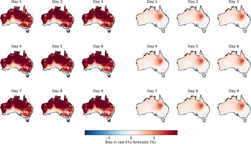
4774           Q. Yang et al.: Bias-correcting input variables enhances forecasting of reference crop evapotranspiration

2016), and high data availability (Er-Raki et al., 2010),             We hypothesize that reducing errors in input variables as
NWP/GCM-based raw ETo forecasts often demonstrate sys-             a precursor will enhance ETo forecast calibration and lead
tematic errors (Turco et al., 2017). Limitations in model algo-    to more skillful calibrated forecasts. To test this hypoth-
rithms, parameterization, and data assimilation often lead to      esis, we compare two calibration strategies that construct
significant errors in raw forecasts of weather variables (Lim      raw ETo forecasts based on the raw (strategy i) or bias-
and Park, 2019; Vogel et al., 2018). As a result, raw ETo          corrected (strategy ii) input variables in calibrating ETo fore-
forecasts calculated directly with the raw forecasts of input      casts across Australia. This study aims to fill a knowledge
weather variables (e.g., temperature, vapor pressure, solar ra-    gap in NWP-based ETo forecasting and develop a calibration
diation, and wind speed) typically demonstrate substantial         strategy to produce more skillful ETo forecasts.
inconsistencies with observations (Medina and Tian, 2020;
Zhao et al., 2019a) and need to be calibrated to improve fore-
cast quality.                                                      2     Method
   Effective calibration aims to correct errors in raw forecasts
and provide unbiased, reliable, and skillful calibrated fore-      2.1    Reference data and forecasts
casts. Theoretically, two different strategies could be adopted
                                                                   In this study, we use the ETo data derived from the Aus-
to achieve this goal in the calibration of ETo forecasts. The
                                                                   tralian Water Availability Project (AWAP)’s gridded data of
first strategy is to construct raw ETo forecasts directly with
                                                                   temperature, vapor pressure, and solar radiation (Jones et
the raw forecasts of the input variables and then calibrate the
                                                                   al., 2007, 2014), as well as wind speed data developed by
derived ETo forecasts. This strategy lumps errors from the in-
                                                                   Mcvicar et al. (2008), as observations for ETo forecast cal-
put variables together in the raw ETo forecasts and corrects
                                                                   ibration. Weather forecasts from the Australian Community
the combined errors directly (Tian and Martinez, 2014; Zhao
                                                                   Climate and Earth System Simulator G2 version (ACCESS-
et al., 2019a). This strategy is straightforward and thus has
                                                                   G2) model are extracted as inputs for the calculation of raw
been adopted by most existing calibrations of NWP/GCM-
                                                                   ETo forecasts. We modify the spatial resolution of ACCESS-
based ETo forecasts. For example, Medina et al. (2018) used
                                                                   G2 forecasts using bilinear interpolation to match the AWAP
a linear regression bias-correction method to calibrate ETo
                                                                   data’s grid spacing. The 3-hourly ACCESS-G2 forecasts dur-
forecasts from three NWP models and achieved significant
                                                                   ing April 2016–March 2019 are aggregated to the daily scale
improvements in forecast quality. Medina and Tian (2020)
                                                                   to match the timeframe of the original site observations used
employed three probabilistic-based calibration methods to
                                                                   to generate the AWAP data. The ACCESS-G2 weather fore-
calibrate ETo forecasts from multiple NWP models, and gen-
                                                                   casts have a forecast horizon of 9 d. AWAP ETo during
erated more skillful and reliable forecasts than using a sim-
                                                                   April 1999–March 2019 is used for the training of the cal-
ple regression bias-correction model. Another probabilistic
                                                                   ibration model, and data during April 2016–March 2019 are
postprocessing method, the Bayesian joint probability (BJP)
                                                                   selected for forecast calibration and evaluation.
model, was adopted to improve the accuracy and skills of
GCM-based ETo forecasts across multiple sites in Australia         2.2    Calculation of ETo
(Zhao et al., 2019a, b).
   Alternatively, ETo forecast calibration could start with cor-   We calculate ETo forecasts and AWAP ETo using the FAO56
recting errors in input variables. Raw forecasts of input vari-    equation (Allen et al., 1998):
ables could be improved first, and raw ETo forecasts could
then be constructed with the corrected input variables. After                                   900
                                                                           0.4081(Rn − G) + γ T +273 u2 (es − ea )
that, the derived raw ETo forecasts could be further improved      ETo =                                             ,         (1)
                                                                                     1 + γ (1 + 0.34u2 )
through calibration. This strategy requires one more step than
the one using the raw input variables. With the improved in-       where ETo is the reference crop evapotranspiration
put variables, errors in the resultant raw ETo forecasts could     (mm d−1 ); 1 is the slope of the vapor pressure curve
be significantly reduced (Nouri and Homaee, 2018; Perera           (kPa ◦ C−1 ); Rn is net radiation at the crop surface
et al., 2014). However, there is no conclusion on whether          (MJ m−2 d−1 ); G is soil heat flux density (MJ m−2 d−1 ); γ
improving raw forecasts of input variables will eventually         is the psychrometric constant (kPa ◦ C−1 ); T is average air
add additional skills to calibrated ETo forecasts (Medina and      temperature (◦ C); u2 is the wind speed at the height of 2 m
Tian, 2020).                                                       (m s−1 ); and es and ea are saturated and actual vapor pressure
   Which calibration strategy produces more skillful cal-          (kPa), respectively.
ibrated forecasts is a critical question in NWP-based                 In constructing raw ETo forecasts, temperature and solar
ETo forecasting, but the answer remains unclear. Since             radiation are readily available from the ACCESS-G2 outputs.
NWP/GCM-based ETo forecasting is increasingly conducted            To obtain the wind speed forecasts, we first use the forecasts
to support water resource management, there is a need to in-       of zonal (u) and meridional (v) components to calculate wind
vestigate the necessity of correcting raw forecasts of the input   speed forecasts at 10 m, and we then estimate wind speed at
variables in ETo forecast calibration.                             2 m using the equation recommended by FAO (Allen et al.,

Hydrol. Earth Syst. Sci., 25, 4773–4788, 2021                                       https://doi.org/10.5194/hess-25-4773-2021
Q. Yang et al.: Bias-correcting input variables enhances forecasting of reference crop evapotranspiration 4775
1998). In addition, we use the ACCESS-G2 forecasts of air 2.3.2 Key steps of ETo forecast calibration using the
pressure and specific humidity to obtain the vapor pressure SCC model
forecasts.
After we construct the raw ETo forecasts, based on either
2.3 Calibration of ETo forecasts raw (calibrations 1 and 3) or bias-corrected (calibrations 2
and 4) forecasts of the input variables, we employ the SCC
The calibration model used in this study is the Seasonally model to further calibrate the ETo forecasts. For the calibra-
Coherent Calibration (SCC) model, which is introduced in tions (calibrations 1 and 2) applying SCC to ETo anomalies,
detail in Sect. 2.3.2. For the calibration across Australia with the first step is to derive the climatological mean at the daily
a spatial resolution of 0.05◦ , we process 281 655 grid cells in scale using the 20-year AWAP ETo. Calibrations 3 and 4 skip
total. We apply the SCC model for ETo forecast calibration this step and apply the SCC model to ETo forecasts directly.
to each grid cell and lead time separately. We use the method developed by Narapusetty et al. (2009)
We conduct four calibrations to evaluate how the two dif- and adopt trigonometric functions and harmonics to simulate
ferent strategies will affect the calibrated ETo forecasts (Ta- the annual cycle of AWAP ETo to derive the climatological
ble 1 and Fig. S1). Our recent investigation suggests calibrat- mean:
ing ETo anomalies, which are calculated as departures from
the climatological mean, could produce more skillful cali- XH
ycm (t) = a0 + a cos wj t + bj sin wj t ,
j =1 j
(2)
brated forecasts than calibrating ETo forecasts directly (Yang
et al., 2021b). As a result, in this study, we primarily focus
on calibrations based on ETo anomalies (calibrations 1 and where ycm (t) is the climatological mean of AWAP ETo at the
2). The comparison between calibrations 1 and 2 is to inves- daily scale; H is the number of harmonics. We use H = 4
tigate whether the bias correction of input variables would following Narapusetty et al. (2009); a0 , aj , and bj are co-
further improve ETo forecasts when the calibration is con- efficients, estimated through minimizing the mean squared
ducted based on ETo anomalies and climatological mean. differences between climatological mean and observations;
We also conduct additional calibrations which postprocess wj = 2πj/P , and P is the number of days in 1 year.
ETo forecasts directly (calibrations 3 and 4) to test whether We then remove the climatological mean from both raw
the contribution of improving input variables to ETo forecast ETo forecasts and AWAP ETo to generate anomalies. We cal-
calibration, if there is any, will depend on how ETo forecasts ibrate the derived anomalies of raw ETo forecasts against
are calibrated (based on anomalies vs. based on ETo). Cal- the anomalies of AWAP ETo using the SCC model. The
ibrations 3 and 4 will help evaluate the general applicabil- SCC model is composed of four key components, includ-
ity of strategy ii to enhance NWP/GCM-based ETo forecast- ing (i) a joint probability model to characterize the connec-
ing. Key steps of the four calibrations could be found in the tion between raw forecasts and observations, (ii) reconstruc-
schematic diagram introducing how raw ETo forecasts are tion of seasonal patterns in raw forecasts based on the long-
constructed and how calibrations are conducted (Fig. S1). In term observations, (iii) reparameterization to obtain param-
the main text, we primarily analyze results from calibrations eters for short-archived raw forecasts, and (iv) generation of
1 and 2. Improvements with the adoption of bias correction calibrated forecasts with the parameters and the joint model.
to input variables in calibrations 3 and 4 are very similar to The SCC model has been introduced in detail in our site- and
calibrations 1 and 2 (see the Supplement). To avoid redun- continental-scale calibrations of NWP precipitation forecasts
dancy, we mainly present results from calibrations 3 and 4 in (Wang et al., 2019; Yang et al., 2021a).
the Supplement. In this study, we use the Yeo–Johnson transformation
method to transform the anomalies of forecasts and refer-
2.3.1 Bias correction of input variables ence data to approach a normal distribution (Yeo and John-
son, 2000):
In ETo forecast calibration employing strategy ii (calibra-
tions 2 and 4), we use a nonparametric quantile mapping
1
(λx + 1) λ − 1, (x ≥ 0, λ 6 = 0)
method (QUANT) to correct raw forecasts of the input vari-
exp (x) − 1, (x ≥ 0, λ = 0)
ables. The QUANT method has been widely used in hydro- x̂ = 1 (3)
logical and climatological investigations to correct bias in
−(λ − 2)x + 1) 2−λ + 1, (x < 0, λ 6 = 2)
− exp (−x) + 1, (x < 0, λ = 2)
raw forecasts (Boe et al., 2007). To use QUANT, we first
build up the empirical cumulative density function (CDF)
of both raw forecasts and AWAP data for each variable. We where λ is a transformation parameter; x refers to anomalies
then calculate the percentile of each record in raw forecasts of daily raw ETo forecasts or AWAP ETo (mm d−1 ); x̂ is the
in their CDF. Next, these percentiles are used to search val- transformed x.
ues in the corresponding AWAP data, which are then treated We assume that the transformed anomalies of ETo fore-
as the bias-corrected forecasts. casts (f (t)) and AWAP ETo (o(t)) are drawn from a bivariate
https://doi.org/10.5194/hess-25-4773-2021 Hydrol. Earth Syst. Sci., 25, 4773–4788, 2021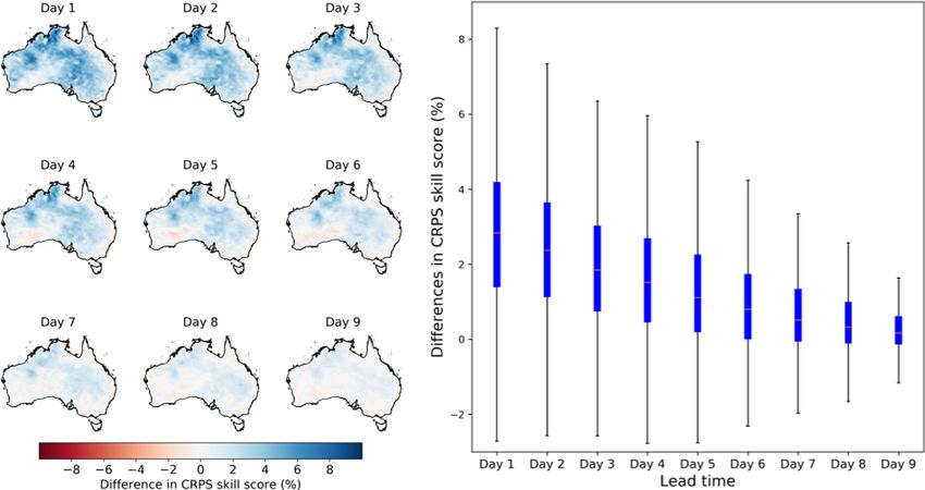
4776            Q. Yang et al.: Bias-correcting input variables enhances forecasting of reference crop evapotranspiration

Table 1. Four sets of ETo forecast calibrations.

         Calibrations     Construction of raw ETo forecasts             Application of the SCC model
         Calibration 1    Raw forecasts of input variables              SCC calibration based on anomaly and climatological mean
         Calibration 2    Bias-corrected forecasts of input variables   SCC calibration based on anomaly and climatological mean
         Calibration 3    Raw forecasts of input variables              The SCC model applied directly to raw ETo forecasts
         Calibration 4    Bias-corrected forecasts of input variables   The SCC model applied directly to raw ETo forecasts

normal (BN) distribution:                                                March 2019) are left out in parameter inference. Optimized
                                                                         parameters are then used to calibrate raw forecasts of this
 f (t) , o (t) ∼ BN(f (t), o(t)|µf (m(t)), σf2 (m(t)),

                                                                         specific month. This process is repeated until all 36 months
µo (m(t)), σo2 (m(t)), ρ(m(t))),                                 (4)     are processed. The cross-validation is to make sure that raw
                                                                         forecasts used to generate calibrated forecasts are not used in
where m(t) returns the month k (k = 1 to 12) of daily fore-              parameter optimization.
casts or observations of day t; µf (m(t)) and σf (m(t)) refer               We also produce climatology forecasts based on the
to the marginal distribution’s mean and standard deviation of            monthly mean and standard deviation parameters of AWAP
f (t) in month m(t), respectively; µo (m(t)) and σo (m(t)) are           ETo (Eq. 4). The randomly sampled climatology is used as
the mean and standard deviation of the marginal distribution             the baseline to evaluate the calibrated ETo forecasts. We
of o (t) in month m(t); ρ(m (t)) is the correlation between              evaluate the calibrations by checking bias, temporal variabil-
f (t) and o (t) of month m(t).                                           ity, skill score, and reliability of the calibrated forecasts. We
   With the long-term (20-year) AWAP ETo data, we can di-                conduct t tests to compare the performance of bias correc-
rectly estimate µo (m(t)) and σo (m(t)) based on a maximum               tion to input variables and the calibrations of ETo forecasts
likelihood optimization. Calculation of the mean (µf (m(t)))             (Tables S1 and S2). The evaluation metrics are further intro-
and standard deviation (σf (m (t))) using the short-archived             duced in detail as follows.
raw ETo (3-year) forecasts is subject to significant sampling
errors. Instead, we indirectly estimate them using the follow-           2.4.1    Bias
ing linear regressions:
                                                                         We evaluate bias of the raw and calibrated forecasts relative
µf (k) = a + bµo (k),                                            (5)     to AWAP ETo using the following equation:
σf (k) = c + dσo (k),                                            (6)              1 XT
ρ(k) = r,                                                        (7)     Bias =      t=1
                                                                                         (x(t) − y(t)),                               (8)
                                                                                  T
where k refers to month of the year (k = 1 to 12); a, b, c, and          where “Bias” refers to the average difference between ETo
d are parameters characterizing the linear relationships; ρ(k)           forecasts and AWAP ETo (mm d−1 ); T is total number
denotes the correlation coefficient between anomalies of raw             of days during the 3-year validation period (April 2016–
forecast and AWAP ETo for each month; and r is the cor-                  March 2019); x(t) is raw or calibrated forecasts of ETo
relation coefficient between anomalies of raw forecasts and              (mm d−1 ); and y(t) is the corresponding AWAP ETo of the
observations in the transformed space (Wang et al., 2019).               same period. Since bias measures the average difference be-
   With the optimized parameters (means, standard devia-                 tween forecasts and observations and could be either possible
tions, and correlations) for the BN distribution (Eq. 4), a con-         and negative, comparing biases of forecasts from different
ditional distribution for o(t) for a given raw forecast (f (t))          calibrations directly will not demonstrate which calibration
is derived. From this conditional distribution, we randomly              has better performance. To solve this problem, we compare
draw 100 samples, which are treated as the calibrated en-                the absolute bias of calibrated forecasts from different cal-
semble forecasts for that raw forecast. Finally, the calibrated          ibrations to evaluate how bias correction of input variables
anomalies are back-transformed to their original space and               affects the accuracy of calibrated ETo forecasts. Lower abso-
added back to the climatological mean to produce calibrated              lute bias indicates smaller differences between forecasts and
ETo forecasts.                                                           AWAP ETo and therefore suggests better performances.

2.4    Evaluation of calibrated forecasts                                2.4.2    Temporal variability

We evaluate the performance of the calibrations using a                  We use the Pearson correlation coefficient (r) between raw
strict leave-one-month-out cross-validation, in which each               and bias-corrected forecasts of input variables and the cor-
of the 36 months during April 2016–March 2019 and the                    responding AWAP data to evaluate how quantile mapping
same month in the 20-year reference data (April 1999 to                  improves the temporal patterns of the input variables. We

Hydrol. Earth Syst. Sci., 25, 4773–4788, 2021                                             https://doi.org/10.5194/hess-25-4773-2021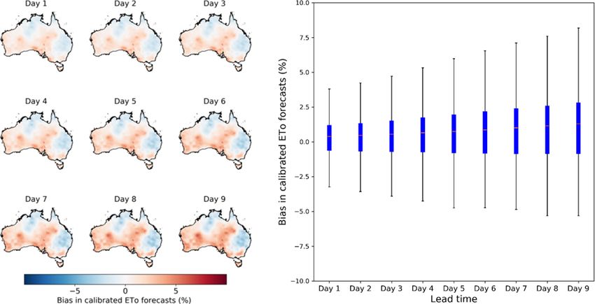
Q. Yang et al.: Bias-correcting input variables enhances forecasting of reference crop evapotranspiration                    4777

also compare the r between raw ETo forecasts (calibrations         2.4.4    Reliability
1 or 3) constructed with raw inputs and AWAP ETo vs. the r
between raw ETo forecasts (calibrations 2 or 4) constructed        We evaluate the reliability of calibrated forecasts using the
with bias-corrected inputs and AWAP ETo. In the evaluation         probability integral transform (PIT) value calculated with the
of calibrated ensemble forecasts, we use the ensemble mean         following equation:
of the 100 ensemble members to calculate r:
            Pn                                                     π (t) = F (t, x = y (t))                                   (13)
               t=1 (x (t) − x)(y (t) − y)
r = qP                      qP                   ,      (9)        where F (t, x) is the cumulative density function of the en-
          n               2     n              2
          t=1 (x (t) −  x)      t=1 (y (t) − y)
                                                                   semble forecast, and y (t) is the AWAP ETo. For reliable
where x(t) is raw or calibrated forecasts; x is the average of     forecasts, π (t) follows a uniform distribution. We use the
x(t); y(t) is the corresponding AWAP ETo data of the same          α index (α) to summarize the reliability in each grid cell
period; and y is the average of y(t).                              with the following equation to check the spatial patterns of
                                                                   forecast reliability (Renard et al., 2010):
2.4.3   Skills of the raw and calibrated forecasts
                                                                              2 Xn              t
                                                                   α = 1−        t=1
                                                                                     π ∗ (t) −                                (14)
We use the continuous ranked probability score (CRPS) to                      n                n+1
measure skills in the raw and calibrated forecasts (Grimit et
                                                                   where π ∗ (t) is the sorted π(t), t = 1, 2, . . . n in ascending
al., 2006):
            Z                                                      order, and n is the total number of days during April 2016–
                                                                   March 2019. The α index measures the total deviation of cal-
CRPS (t) = {F (t, x) − H (x − y (t))}2 dx,              (10)
                                                                   ibrated forecasts from the corresponding uniform quantile.
          1 XT                                                     Perfectly reliable forecasts should have an α of 1, and fore-
CRPS =           t=1
                     CRPS (t) ,                           (11)     casts with no reliability would have an α of 0.
          T
                                                                      We further evaluate the reliability of calibrated ETo fore-
where F (t, x) is the cumulative density function of an en-
                                                                   casts from calibration 2 using the reliability diagram (Hart-
semble forecast, and y (t) is the observation at time t; H
                                                                   mann et al., 2002), which assesses how well the predicted
is the Heaviside step function (H = 1 if x − y (t) ≥ 0 and
                                                                   probabilities of forecasts match observed frequencies. We
H = 0 otherwise); the overbar represents averaging across
                                                                   convert the calibrated ensemble ETo forecasts to forecast
the T days. For deterministic forecasts, CRPS is reduced to
                                                                   probabilities exceeding three thresholds, including 3, 6, and
absolute errors.
                                                                   9 mm d−1 . We pool forecasts of different grid cells, days,
   We further calculate the CRPS skill score (CRPSSS ) to
                                                                   and lead times together in the calculation of forecast proba-
measure the skills relative to climatology forecasts using the
                                                                   bility. In the reliability diagram, perfectly reliable forecasts
following equation:
                                                                   would demonstrate a curve along the diagonal. A plotted
            CRPSreference − CRPSforecasts                          curve above the diagonal indicates underestimations and vice
CRPSSS =                                  × 100,           (12)
                  CRPSreference                                    versa.
where CRPSreference is the CRPS value of climatology fore-
casts ( %); CRPSforecasts refers to CRPS value of raw or cali-     3     Results
brated forecasts.
   In the calculation of CRPS skill score, both climatol-          3.1     Quality of raw and bias-corrected input variables
ogy forecasts or the last observations (persistence) have
been used as reference forecasts (Pappenberger et al., 2015;       Raw forecasts of the five input variables demonstrate sig-
Thiemig et al., 2015). However, reference forecasts based on       nificant inconsistencies with the corresponding AWAP data
persistence are more suitable for evaluating the performance       (Figs. S2–S6). In most parts of Australia, raw daily maxi-
of forecasts shorter than 2 d. As a result, we choose climatol-    mum temperature (Tmax ) forecasts are lower than AWAP data
ogy forecasts as the reference, since errors in climate fore-      by 1–2 ◦ C. Overpredictions in Tmax are only found in coastal
casts are similar among all lead times and thus could be used      areas of northwestern Australia. The daily minimum temper-
to demonstrate the increasing errors in raw and calibrated         ature (Tmin ) is underpredicted by more than 1.5 ◦ C in western
forecasts as lead time advances. For CRPSSS of calibrations        and central parts of Australia by the raw forecasts, but it is
1 and 2, climatology forecasts from calibration 1 are used;        overpredicted by ca. 1 ◦ C in eastern and southern Australia.
For CRPSSS of calibrations 3 and 4, climatology forecasts          Vapor pressure is underpredicted in western and central re-
from calibration 3 are used. Positive skill scores indicate bet-   gions by ca. 14 %, but it is overpredicted by ca. 6 % in coastal
ter skills than the climatology forecasts and vice versa. We       areas of southeastern Australia by the raw forecasts. Raw
use percentage as the unit of CRPS skill score, so low skill       solar radiation forecasts are about 5 % higher than AWAP
scores at long lead times will be converted from small deci-       data across Australia. Forecasted wind speed is higher than
mals to more readable percent.                                     the reference data by more than 1 m s−1 (or by ca. 63 %) in

https://doi.org/10.5194/hess-25-4773-2021                                          Hydrol. Earth Syst. Sci., 25, 4773–4788, 2021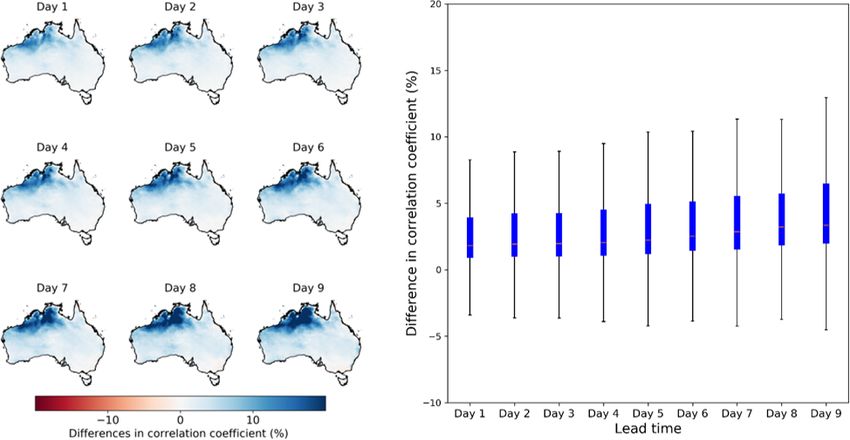
4778           Q. Yang et al.: Bias-correcting input variables enhances forecasting of reference crop evapotranspiration

most parts of Australia. For each input variable, spatial pat-     ity in the calculation of ETo using the input variables, spa-
terns of biases in raw forecasts are consistent across the nine    tial patterns of improvements in r (Fig. 2) does not resemble
lead times, demonstrating systematic errors in the raw NWP         improvements in any individual input variables (Figs. S7 to
forecasts. According to our statistical test, overpredictions or   S11). The improvements in r of raw ETo forecasts seem to
underpredictions in raw forecasts of the input variables are       be contributed jointly by these input variables and their inter-
statistically significant (P 0.9) than      ETo forecasts (Fig. 3). The calibrated ETo forecasts from cal-
the other three variables, and wind speed forecasts demon-         ibration 2 show low biases close to zero across all grid cells
strate the lowest correlations with AWAP data. For all vari-       and lead times. Overpredictions in Queensland in the raw
ables, the r decreases with lead time, indicating higher un-       ETo forecasts calculated with the bias-corrected input vari-
certainties at long lead times in raw forecasts.                   ables are effectively corrected (Figs. 1, 3, and S12), leading
   Quantile mapping effectively corrects biases in raw fore-       to lower biases in the calibrated forecasts. According to the
casts of the input variables. Through the bias correction, sig-    t test (Table S2), biases of calibrated forecasts at the first two
nificant overpredictions and underpredictions in raw fore-         lead times are not significantly different from zero, indicating
casts of the five variables are significantly reduced, result-     the effective bias reduction through calibration 2. For the re-
ing in biases close to zero for all lead times across Aus-         maining seven lead times (days 3 to 9), the overall biases are
tralia (Figs. S2–S6). In addition, quantile mapping also im-       slightly higher than zero. The remaining biases in calibrated
proves the correlation between forecasts of input variables        forecasts reflect deviations of ETo during the evaluation pe-
and AWAP data (Figs. S7–S11). The most significant im-             riod (April 2016–March 2019) from the climatology during
provements are found in wind speed forecasts, in which the         April 1999–March 2019, since the SCC parameters are in-
r is improved by up to 0.2 in central and southern parts of        ferred with the 20-year AWAP ETo (Eqs. 4 to 7).
Australia. Forecasts of Tmax and solar radiation also demon-          Compared with the calibration constructing raw ETo fore-
strate higher r with the adoption of quantile mapping. Both        casts with raw forecasts of input variables (calibration 1), the
increases and slight decreases were found for vapor pressure       postprocessing based on bias-corrected input variables (cal-
and Tmin , indicating less significant improvements in tempo-      ibration 2) produces more accurate calibrated ETo forecasts
ral patterns than other variables.                                 (Fig. 4). Specifically, calibrated ETo forecasts from calibra-
                                                                   tion 2 demonstrate significantly smaller (P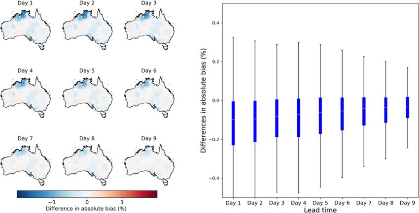
Q. Yang et al.: Bias-correcting input variables enhances forecasting of reference crop evapotranspiration 4779
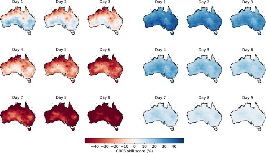
Figure 1. Bias in (three columns on the left) raw ETo forecasts constructed with raw forecasts of input variables and (three columns on the
right) raw ETo forecasts constructed with bias-corrected input variables.
Figure 2. The comparison between the correlation coefficient of raw ETo forecasts constructed with the bias-corrected inputs and AWAP
ETo vs. the correlation coefficient of raw ETo forecasts constructed with the raw inputs and AWAP ETo. The boxplot on the right summarizes
results across all grid cells.
Coastal areas of northern Australia have lower r values than The adoption of bias correction to raw forecasts of input
other regions of the country, demonstrating higher uncertain- variables results in better representation of ETo variability in
ties in ETo forecasts this area. Deficiencies in ACCESS mod- calibrated ETo forecasts (Fig. 6 and Table S2). Increases in
els in simulating dynamics of tropical climate systems may r are particularly significant for short lead times (Table S2).
have resulted in the low r in northern Australia. Specifically, for the first three lead times, increases in r are
mainly around 2 % in central and northern parts of Australia,
https://doi.org/10.5194/hess-25-4773-2021 Hydrol. Earth Syst. Sci., 25, 4773–4788, 2021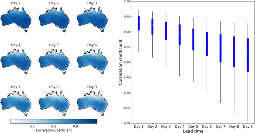
4780            Q. Yang et al.: Bias-correcting input variables enhances forecasting of reference crop evapotranspiration

Figure 3. Bias in calibrated ETo forecasts from calibration 2, in which raw ETo forecasts are constructed with bias-corrected input variables.
Maps on the left show the spatial patterns of bias, and the boxplot on the right summarizes biases across all grid cells.

Figure 4. Differences in absolute bias between calibrated ETo forecasts from calibration 2 with calibration 1. Maps on the left show the
spatial patterns of difference in absolute bias, and the boxplot on the right summarizes results across all grid cells.

with more pronounced (>4 %) increases found in coastal re-               r of raw ETo forecasts with the adoption of bias correction
gions of the Northern Territory. For lead times 4 to 6, in-              (Fig. 2), particularly for the short lead times. The improve-
creases in r values are mainly above 1 %. For the remaining              ments in r of calibrated ETo forecasts (Fig. 6) may also lead
three lead times (7 to 9), increases in r are mainly located in          to more reasonable conditional distributions for a given raw
Northern Territory. Spatial patterns of r increases from cali-           forecast (Eq. 4). As a result, regions showing improvements
bration 1 to calibration 2 are consistent across the nine lead           in r in calibrated ETo forecasts (Fig. 6) often demonstrate
times.                                                                   reductions in absolute bias (Fig. 4).
   Spatial patterns of improvements in r in calibrated ETo
forecasts (Fig. 6) are consistent with the improvements in

Hydrol. Earth Syst. Sci., 25, 4773–4788, 2021                                               https://doi.org/10.5194/hess-25-4773-2021
Q. Yang et al.: Bias-correcting input variables enhances forecasting of reference crop evapotranspiration 4781
Figure 5. The correlation coefficient between calibrated ETo forecasts from calibration 2 and AWAP ETo. Maps on the left show the spatial
patterns of r, and the boxplot on the right summarizes results across all grid cells.
Figure 6. Differences in the correlation coefficients between calibrated forecasts from calibration 2 and AWAP ETo vs. calibration 1. Maps
on the left show the spatial patterns of differences in r, and the boxplot on the right summarizes results across all grid cells.
3.5 Improvements in forecast skills casts are worse than randomly sampled climatology. Skills in
raw ETo forecasts decrease quickly with lead time. Regions
The calibration of ETo forecasts with the SCC model signif- with positive skills shrink substantially at lead times 3 and 4
icantly improves forecast skills. The raw ETo forecasts cal- and disappear at longer lead times. At lead time 9, skills of
culated with bias-corrected input variables demonstrate low raw forecasts are mainly below −40 %.
skills, even at short lead times (Figs. 7 and S13). Specifically, The calibration significantly improves forecast skills
for the first two lead times, central and southern Australia across all lead times (Table S2). Calibrated ETo forecasts
show skills better than the climatology forecasts by 10 % to from calibration 2 show CRPS skill scores above 35 % at lead
20 %. However, in most parts of northern Australia, raw fore- time 1 across Australia, and the skills are generally above
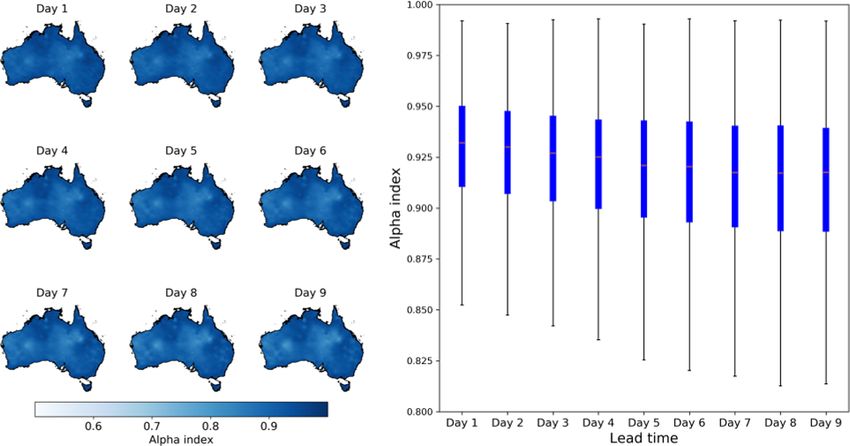
https://doi.org/10.5194/hess-25-4773-2021 Hydrol. Earth Syst. Sci., 25, 4773–4788, 20214782 Q. Yang et al.: Bias-correcting input variables enhances forecasting of reference crop evapotranspiration Figure 7. CRPS skill score in the (three columns on the left) raw ETo forecasts calculated with bias-corrected input variables and (three columns on the right) calibrated forecasts from calibration 2. 30 % at lead times 2 and 3. Since ETo forecasts have been reliable ensemble spreads in calibrated forecasts across all widely used to inform real-time decision-making for farm- lead times. In most grid cells, the α index is over 0.9, in- ing, high skills in calibrated ETo forecasts for the short lead dicating reasonable representations of ETo uncertainties by times are expected to be highly valuable for activities such as the ensemble spread, which is neither too narrow nor too irrigation scheduling. Although skills of calibrated forecasts wide (Fig. 9). Calibrated forecasts from calibration 1, which also decrease with lead time, they remain above zero at long uses raw input variables, demonstrate similar reliability as lead times (Figs. 7 and S13). those from the calibration with bias-corrected input vari- We further compare skills of calibrated ETo forecasts be- ables (calibration 2). Differences in α index of the calibrated tween calibrations 2 and 1 (Fig. 8). We achieve significant in- ETo forecasts from calibrations 1 and 2 are almost negligi- creases (P
Q. Yang et al.: Bias-correcting input variables enhances forecasting of reference crop evapotranspiration                              4783

Figure 8. Differences in CRPS skill score between the calibrated ETo forecasts from calibration 2 with those from calibration 1. Maps on
the left show the spatial patterns of difference in CRPS skill score, and the boxplot on the right summarizes results across all grid cells.

Figure 9. The α index of calibrated ETo ensemble forecasts from calibration 2. Maps on the left show the spatial patterns of the α index, and
the boxplot on the right summarizes results across all grid cells.

score in terms of magnitude, spatial patterns, and trend along           3.8   Summary of results
the lead times, when ETo forecasts are calibrated directly
(Figs. S15–S17). In addition, the α index was only slightly
different between calibrations 3 and 4 (Fig. S18). This addi-            Although the selected metrics measure different aspects
tional comparison further confirms the general applicability             of forecast quality, they generally agree with each other
of strategy ii for enhancing NWP-based ETo forecasting.                  in demonstrating improvements in calibrated ETo forecasts
                                                                         with the adoption of the strategy ii. As introduced in the
                                                                         Method section, bias measures average differences; corre-
                                                                         lation coefficient shows consistency between observations

https://doi.org/10.5194/hess-25-4773-2021                                              Hydrol. Earth Syst. Sci., 25, 4773–4788, 2021
4784 Q. Yang et al.: Bias-correcting input variables enhances forecasting of reference crop evapotranspiration
Figure 10. Reliability diagrams of calibrated ETo forecasts during April 2016–March 2019 with thresholds of 3, 6, and 9 mm d−1 .
and forecasts in temporal variability; the CRPS skill score casts (3-year vs. 23-year) than Zhao et al. (2019a). Cali-
measures the performance of the calibrated forecasts relative brated forecasts from calibration 2 also demonstrate low bi-
to climatology forecast; the α index is an indicator show- ases (0.32 %–0.95 %) comparable with calibrated ETo fore-
ing whether the distribution of calibrated forecasts is over- casts (0.49 %–0.63 %) based on the Bayesian model averag-
confident or underconfident. As a result, these metrics may ing (BMA) model and weather forecasts from three NWP
differ from each other in magnitude when used to evaluate models in the USA during 2014–2016 (Medina and Tian,
different calibrations (Figs. 4, 6, 8, and S14). However, im- 2020).
provements in bias, correlation, and skills with the adoption This investigation also contributes to filling a knowl-
of bias correction to input variables are generally consistent edge gap in NWP-based ETo forecasting. Although previous
in spatial patterns. Compared with the other three metrics, α calibrations using raw forecasts of input variables to con-
index demonstrates less significant changes when input vari- struct the raw ETo forecasts (strategy i) for calibration of-
ables are bias corrected first (Table S2 and Fig. S14), mainly ten achieved significant improvements in skills, it is unclear
because this index is less sensitive to changes in calibrated whether improving forecasts of input variables could further
forecasts than other metrics. enhance ETo forecast calibration (Medina and Tian, 2020).
How the raw ETo forecasts should be constructed represents
a critical knowledge gap in the area of NWP-based ETo fore-
4 Discussion casting (Medina and Tian, 2020). Results of this investiga-
tion provide strong evidence for the necessity of improving
4.1 Importance of improving forecasts of input input variables prior to constructing raw ETo forecasts. The
variables for NWP-based ETo forecasting nonlinear and nonstationary behaviors of the input variables
used for ETo calculation have been reported (Paredes et al.,
This investigation further highlights the importance of sta- 2018). This study suggests that when raw input variables are
tistical calibration in NWP-based ETo forecasting (Medina used to construct the raw ETo forecasts, complex interac-
and Tian, 2020). According to an investigation across 40 sites tions among these variables may lead to errors in raw ETo
in Australia, raw ETo forecasts constructed with NWP out- forecasts that could not be effectively corrected through sta-
puts reasonably captured the magnitude and variability of tistical calibration. Bias correction of input variables could
ETo, but forecast skills better than climatology were only help prohibit the propagation of errors from input variables
limited to the first six lead times (Perera et al., 2014). Our to ETo forecasts (Zappa et al., 2010), as evidenced by the
investigation suggests that statistical calibration could sub- higher accuracy and higher skills in calibrated ETo forecasts
stantially improve forecast skills and successfully extend the when input variables are bias corrected. In addition, a further
skillful forecasts to lead time 9 across Australia. Findings evaluation based on a different way of implementing the SCC
of this investigation agree well with the site-scale short- model demonstrates similar improvements in calibrated ETo
term ETo forecasting based on GCM outputs (Zhao et al., forecasts with the adoption of bias correction to input vari-
2019a) in the improvements of forecast skills through sta- ables (calibrations 3 and 4). Results from calibrations 3 and
tistical calibration. Calibrated forecasts from calibration 2 4 further confirm that additional skills have been added to
demonstrate similar skills as Zhao et al. (2019a) across three raw ETo forecasts through the bias correction of input vari-
Australian sites. Thanks to the capability of SCC in calibrat- ables, and the improvements to calibrated ETo forecasts tend
ing short-archived forecasts (Wang et al., 2019), we achieve to be independent of calibration models. Consequently, we
the improvements based on much shorter archived raw fore- anticipate that future NWP-based ETo forecasting could ben-
Hydrol. Earth Syst. Sci., 25, 4773–4788, 2021 https://doi.org/10.5194/hess-25-4773-2021Q. Yang et al.: Bias-correcting input variables enhances forecasting of reference crop evapotranspiration 4785
efit from adopting this calibration strategy to produce more will be improved using strategy ii but based on a different
skillful calibrated ETo forecasts. calibration model. In addition, we use bilinear interpolation
to match the NWP forecasts and AWAP data. More sophisti-
4.2 Implications for forecasting of integrated variables cated remapping methods should be evaluated to understand
and future work the impacts of forecast regridding on statistical calibration.
The applicability of the calibration strategy developed in
This investigation also provides valuable implications for the this study to seasonal ETo forecasting should be further in-
forecasting of integrated variables, which are derived based vestigated. Seasonal ETo forecasting based on GCM climate
on multiple NWP/GCM variables. Variables such as drought forecast has been increasingly performed (Tian et al., 2014;
index (Zhang et al., 2017), bushfire danger index (Sharples Zhao et al., 2019b). In these investigations, raw ETo forecasts
et al., 2009), and severe weather index (Rabbani et al., 2020) were also constructed directly with raw GCM climate fore-
are often derived by combining multiple weather variables casts. As a result, it is expected that these investigations have
produced by NWP models. Our investigation suggests that suffered from error propagation from input variables to sea-
improving the input variables could effectively reduce error sonal ETo forecasts. Whether the calibration strategy (strat-
propagation from inputs to integrated variables. This extra egy ii) developed in this study will be applicable to seasonal
step is proven to be particularly useful in reducing errors in ETo forecasting warrants further investigations.
the integrated variables that could not be corrected through
calibration. We anticipate that this extra step could help im-
prove the predictability of integrated variables. 5 Conclusions
Although we have conducted thorough analyses on the
NWP outputs have been increasingly used for ETo forecast-
contribution of improving input variables to ETo forecast cal-
ing to support water resource management. Statistical cal-
ibration, further investigations will be needed to validate the
ibration plays an essential role in improving the quality of
robustness of findings in this study. First, we anticipate that
ETo forecasts. However, it is unclear whether improving raw
the ETo forecasts could be further improved if a more sophis-
forecasts of input variables is necessary for the calibration of
ticated calibration model is applied to raw forecasts of the in-
ETo forecasts. We aim to fill this knowledge gap through a
put variables. In this study, we adopt a simple bias-correction
thorough comparison of two calibration strategies in the cal-
method to improve the input variables. Limitations of quan-
ibration of NWP-based ETo forecasts.
tile mapping have been reported in previous studies (Schepen
This investigation clearly suggests the necessity of im-
et al., 2020; Zhao et al., 2017). Our analyses demonstrate
proving input variables as part of ETo forecast calibration.
that the raw ETo forecasts calculated with the bias-corrected
With this extra step, the bias, correlation coefficient, and
input variables still show low forecast skills, particularly at
skills of the calibrated ETo forecasts are all improved. Fur-
long lead times (Fig. 7). If a more sophisticated calibration
ther investigation indicates that the improvements tend to
method is employed to the input variables, error propagation
be independent of the calibration method applied to ETo
from input variables to ETo forecasts will likely be further re-
forecasts. Forecasting the highly variable ETo is often chal-
duced. As a result, we anticipate that the calibrated ETo fore-
lenging. This investigation addresses a common challenge in
cast will gain further improvements in forecast skills. An-
NWP-based ETo forecasting and develops an effective cali-
other advantage of correcting input variables with a sophisti-
bration strategy for adding extra skills to ETo forecasts. We
cated model is that it will produce a set of skillful calibrated
anticipate that future NWP-based ETo forecasting could ben-
weather forecasts. Well-calibrated forecasts of temperature,
efit from adopting this strategy to produce more skillful cal-
vapor pressure, solar radiation, and wind speed could be use-
ibrated ETo forecasts. This strategy is also expected to be
ful for forecast users such as crop modelers and bushfire
applicable to enhancing the forecasting of other integrated
managers.
variables that are calculated using multiple NWP/GCM vari-
Second, the two calibration strategies should be tested us-
ables as inputs.
ing other NWP models. In this study, we use one NWP model
to investigate a critical knowledge gap in NWP-based ETo
forecasting. Additional investigations are needed to examine Data availability. Data used in this study are available by contact-
whether improvements achieved with the adoption of calibra- ing the corresponding author.
tion strategy ii will hold for ETo forecasting based on other
NWP models. Third, further investigations based on other
calibration models are needed to validate findings of this Supplement. The supplement related to this article is available on-
investigation. Our analyses based on two different methods line at: https://doi.org/10.5194/hess-25-4773-2021-supplement.
(based on ETo anomalies vs. based on original ETo) demon-
strate similar improvements in calibrated ETo forecasts with
the adoption of bias correction to input variables. Additional Author contributions. QY and QJW conceived this study. QJW de-
evaluations will be needed to verify whether forecast skills veloped the calibration model. QY took the lead in writing and
https://doi.org/10.5194/hess-25-4773-2021 Hydrol. Earth Syst. Sci., 25, 4773–4788, 20214786 Q. Yang et al.: Bias-correcting input variables enhances forecasting of reference crop evapotranspiration
improving the article. All co-authors, including KH and YT, con- ity of Maize from Meteorological Data under Semiarid Climate,
tributed to discussing the results and improving this study. Water, 10, 1–17, https://doi.org/10.3390/w10040405, 2018.
Er-Raki, S., Chehbouni, A., Khabba, S., Simonneaux, V., Jar-
lan, L., Ouldbba, A., Rodriguez, J. C., and Allen, R.: Assess-
Competing interests. The authors declare that they have no conflict ment of reference evapotranspiration methods in semi-arid re-
of interest. gions: Can weather forecast data be used as alternate of ground
meteorological parameters?, J. Arid Environ., 74, 1587–1596,
https://doi.org/10.1016/j.jaridenv.2010.07.002, 2010.
Disclaimer. Publisher’s note: Copernicus Publications remains Grimit, E. P., Gneiting, T., Berrocal, V. J., and Johnson, N.
neutral with regard to jurisdictional claims in published maps and A.: The continuous ranked probability score for circular
institutional affiliations. variables and its application to mesoscale forecast ensem-
ble verification, Q. J. Roy. Meteor. Soc., 132, 2925–2942,
https://doi.org/10.1256/qj.05.235, 2006.
Hartmann, H., Pagano, T. C., Sorooshian, S., and Bales, R.: Evaluat-
Acknowledgements. Computations for this research were under-
ing Seasonal Climate Forecasts from User Perspectives, B. Am.
taken with the assistance of resources and services from the Na-
Meteorol. Soc., 83, 683–698, 2002.
tional Computational Infrastructure (NCI), which is supported by
Hopson, T. M. and Webster, P. J.: A 1–10-Day Ensemble Forecast-
the Australian Government. This research was supported by the
ing Scheme for the Major River Basins of Bangladesh: Forecast-
“Sustaining and strengthening merit-based access to National Com-
ing Severe Floods of 2003–07, J. Hydrometeorol., 11, 618–641,
putational Infrastructure” (NCI) LIEF grant (LE190100021) and fa-
https://doi.org/10.1175/2009JHM1006.1, 2009.
cilitated by The University of Melbourne.
Jones, D. A., Wang, W., and Fawcett, R.: Climate Data for the Aus-
tralian Water Availability Project, Australian Bureau of Meteo-
rology, Melbourne, Australia, available at: https://trove.nla.gov.
Financial support. This research has been supported by the Aus- au/work/17765777?q&versionId=20839991 (last access: 10 De-
tralian Research Council (grant no. LP170100922) and the Aus- cember 2019), 2007.
tralian Bureau of Meteorology (grant no. TP707466). Jones, D. A., Wang, W., and Fawcett, R.: Australian Water
Availability Project Daily Gridded Rainfall, available at: http:
//www.bom.gov.au/jsp/awap/rain/index.jsp (last access: 10 Jan-
Review statement. This paper was edited by Nadia Ursino and re- uary 2020), 2014.
viewed by three anonymous referees. Karbasi, M.: Forecasting of Multi-Step Ahead Reference Evap-
otranspiration Using Wavelet-Gaussian Process Regression
Model, Water Resour. Manag., 32, 1035–1052, 2018.
Kumar, R., Jat, M. K., and Shankar, V.: Methods to estimate irri-
gated reference crop evapotranspiration – a review, Water Sci.
References Technol., 66, 525–535, https://doi.org/10.2166/wst.2012.191,
2012.
Allen, R. G., Pereira, L. S., Raes, D., and Smith, M.: FAO Irrigation Lim, J. and Park, H.: H Filtering for Bias Correction in Post-
and drainage paper No.56, Crop evapotranspiration: guidelines Processing of Numerical Weather Prediction, J. Meteorol.
for computing crop water requirements, Food and Agriculture Soc. Japan, 97, 773–782, https://doi.org/10.2151/jmsj.2019-041,
Organization of the United Nations (FAO), Rome, Italy, 1998. 2019.
Bachour, R., Maslova, I., Ticlavilca, A. M., Walker, W. R., and Mc- Liu, Y. J., Chen, J., and Pang, T.: Analysis of Changes in
kee, M.: Wavelet-multivariate relevance vector machine hybrid Reference Evapotranspiration, Pan Evaporation, and Actual
model for forecasting daily evapotranspiration, Stoch. Environ. Evapotranspiration and Their Influencing Factors in the North
Res. Risk Assess., 30, 103–117, https://doi.org/10.1007/s00477- China Plain During 1998–2005, Earth Sp. Sci., 6, 1366–1377,
015-1039-z, 2016. https://doi.org/10.1029/2019EA000626, 2019.
Ballesteros, R., Ortega, F., and Angel, M.: FORETo: New software Luo, Y., Chang, X., Peng, S., Khan, S., Wang, W., Zheng,
for reference evapotranspiration forecasting, J. Arid Environ., Q., and Xueliang, C.: Short-term forecasting of daily refer-
124, 128–141, https://doi.org/10.1016/j.jaridenv.2015.08.006, ence evapotranspiration using the Hargreaves-Samani model
2016. and temperature forecasts, Agric. Water Manag., 136, 42–51,
Boe, J., Terray, L., Habets, F., and Martin, E.: Statistical https://doi.org/10.1016/j.agwat.2014.01.006, 2014.
and dynamical downscaling of the Seine basin climate for Mariito, M. A., Tracy, J. C., and Taghavv, S. A.: Forecasting of ref-
hydro-meteorological studies, Int. J. Clim., 27, 1463–1655, erence crop evapotranspiration, Agric. Water Manag., 24, 163–
https://doi.org/10.1002/joc.1602, 2007. 187, 1993.
Cai, J., Liu, Y., Lei, T., and Pereira, S. L.: Estimating reference evap- Mcvicar, T. R., Niel, T. G. Van, Li, L. T., Roderick, M. L.,
otranspiration with the FAO Penman – Monteith equation using Rayner, D. P., Ricciardulli, L., and Donohue, R. J.: Wind
daily weather forecast messages, Agric. For. Meteorol., 145, 22– speed climatology and trends for Australia, 1975–2006: Cap-
35, https://doi.org/10.1016/j.agrformet.2007.04.012, 2007. turing the stilling phenomenon and comparison with near-
Djaman, K., Neill, M. O., Owen, C. K., Smeal, D., Koudahe, K., surface reanalysis output, Geophys. Res. Lett., 35, 1–6,
West, M., Allen, S., Lombard, K., and Irmak, S.: Crop Evapo- https://doi.org/10.1029/2008GL035627, 2008.
transpiration, Irrigation Water Requirement and Water Productiv-
Hydrol. Earth Syst. Sci., 25, 4773–4788, 2021 https://doi.org/10.5194/hess-25-4773-2021Q. Yang et al.: Bias-correcting input variables enhances forecasting of reference crop evapotranspiration 4787 Medina, H. and Tian, D.: Comparison of probabilistic post- Sharples, J. J., Mcrae, R. H. D., Weber, R. O., and processing approaches for improving numerical weather Gill, A. M.: A simple index for assessing fire dan- prediction-based daily and weekly reference evapotranspi- ger rating, Environ. Model. Softw., 24, 764–774, ration forecasts, Hydrol. Earth Syst. Sci., 24, 1011–1030, https://doi.org/10.1016/j.envsoft.2008.11.004, 2009. https://doi.org/10.5194/hess-24-1011-2020, 2020. Srivastava, P. K., Han, D., Ramirez, M. A. R., and Islam, T.: Medina, H., Tian, D., Srivastava, P., Pelosi, A., and Chirico, Comparative assessment of evapotranspiration derived from G. B.: Medium-range reference evapotranspiration forecasts NCEP and ECMWF global datasets through Weather Re- for the contiguous United States based on multi-model search and Forecasting model, Atmos. Sci. Lett., 14, 118–125, numerical weather predictions, J. Hydrol., 562, 502–517, https://doi.org/10.1002/asl2.427, 2013. https://doi.org/10.1016/j.jhydrol.2018.05.029, 2018. Thiemig, V., Bisselink, B., Pappenberger, F., and Thielen, J.: A pan- Mushtaq, S., Reardon-smith, K., Kouadio, L., Attard, S., Cobon, African medium-range ensemble flood forecast system, Hydrol. D., and Stone, R.: Value of seasonal forecasting for sugar- Earth Syst. Sci., 19, 3365–3385, https://doi.org/10.5194/hess-19- cane farm irrigation planning, Eur. J. Agron., 104, 37–48, 3365-2015, 2015. https://doi.org/10.1016/j.eja.2019.01.005, 2019. Tian, D. and Martinez, C. J.: The GEFS-Based Daily Reference Narapusetty, B., Delsole, T., and Tippett, M. K.: Optimal esti- Evapotranspiration (ETo) Forecast and Its Implication for Water mation of the climatological mean, J. Climate, 22, 4845–4859, Management in the Southeastern United States, J. Hydrometeo- https://doi.org/10.1175/2009JCLI2944.1, 2009. rol., 15, 1152–1165, https://doi.org/10.1175/JHM-D-13-0119.1, Nouri, M. and Homaee, M.: On modeling reference crop evapotran- 2014. spiration under lack of reliable data over Iran, J. Hydrol., 566, Tian, D., Martinez, C. J., and Graham, W. D.: Seasonal Predic- 705–718, https://doi.org/10.1016/j.jhydrol.2018.09.037, 2018. tion of Regional Reference Evapotranspiration Based on Climate Pappenberger, F., Ramos, M. H., Cloke, H. L., Wetterhall, F., Forecast System Version 2, J. Hydrometeorol., 15, 1166–1188, Alfieri, L., Bogner, K., Mueller, A., and Salamon, P.: How https://doi.org/10.1175/JHM-D-13-087.1, 2014. do I know if my forecasts are better? Using benchmarks in Torres, A. F., Walker, W. R., and Mckee, M.: Forecasting hydrological ensemble prediction, J. Hydrol., 522, 697–713, daily potential evapotranspiration using machine learning and https://doi.org/10.1016/j.jhydrol.2015.01.024, 2015. limited climatic data, Agric. Water Manag., 98, 553–562, Paredes, P., Fontes, J. C., Azevedo, E. B., and Pereira, L. S.: Daily https://doi.org/10.1016/j.agwat.2010.10.012, 2011. reference crop evapotranspiration with reduced data sets in the Turco, M., Ceglar, A., Prodhomme, C., Soret, A., Toreti, A., and humid environments of Azores islands using estimates of actual Francisco, J. D.-R.: Summer drought predictability over Europe: vapor pressure, solar radiation, and wind speed, Theor. Appl. Cli- empirical versus dynamical forecasts, Environ. Res. Lett., 12, matol. Appl., 134, 1115–1133, 2018. 084006, https://doi.org/10.1088/1748-9326/aa7859, 2017. Pelosi, A., Medina, H., Villani, P., D’Urso, G., and Chirico, G. B.: Vogel, P., Knippertz, P., Fink, A. H., Schlueter, A., and Gneiting, Probabilistic forecasting of reference evapotranspiration with a T.: Skill of global raw and postprocessed ensemble predictions limited area ensemble prediction system, Agric. Water Manag., of rainfall over northern tropical Africa, Weather Forecast., 33, 178, 106–118, https://doi.org/10.1016/j.agwat.2016.09.015, 369–388, https://doi.org/10.1175/WAF-D-17-0127.1, 2018. 2016. Wang, Q. J., Zhao, T., Yang, Q., and Robertson, D.: A Seasonally Perera, K. C., Western, A. W., Nawarathna, B., and George, B.: Coherent Calibration (SCC) Model for Postprocessing Numer- Forecasting daily reference evapotranspiration for Australia us- ical Weather Predictions, Mon. Weather Rev., 147, 3633–3647, ing numerical weather prediction outputs, Agric. For. Meteorol., https://doi.org/10.1175/MWR-D-19-0108.1, 2019. 194, 50–63, https://doi.org/10.1016/j.agrformet.2014.03.014, Yang, Q., Wang, Q. J., and Hakala, K.: Achieving ef- 2014. fective calibration of precipitatioAn forecasts over a Perera, K. C., Western, A. W., Robertson, R. D., George, B., continental scale, J. Hydrol. Reg. Stud., 35, 100818, and Nawarathna, B.: Ensemble forecasting of short-term system https://doi.org/10.1016/j.ejrh.2021.100818, 2021a. scale irrigation demands using real-time flow data and numer- Yang, Q., Wang, Q. J., and Hakala, K.: Working with anomalies ical weather predictions, Water Resour. Res., 52, 4801–4822, improves forecast calibration of daily reference crop evapotran- https://doi.org/10.1002/2015WR018532, 2016. spiration, J. Hydrol., in revision, 2021b. Rabbani, G., Yazd, N. K., Reza, M., and Daneshvar, M.: Yeo, I. and Johnson, R. A.: A new family of power transforma- Factors affecting severe weather threat index in urban ar- tions to improve normality or symmetry, Biometrika, 87, 954– eas of Turkey and Iran, Environ. Syst. Res., 9, 1–14, 959, 2000. https://doi.org/10.1186/s40068-020-00173-6, 2020. Zappa, M., Beven, K. J., Bruen, M., Cofino, A. S., Kok, K., Mar- Renard, B., Kavetski, D., Kuczera, G., Thyer, M., and Franks, S. W.: tin, E., Nurmi, P., Orfila, B., Roulin, E., Schroter, K., Seed, A., Understanding predictive uncertainty in hydrologic modeling: Szturc, J., Vehvilainen, B., Germann, U., and Rossa, A.: Propaga- The challenge of identifying input and structural errors, Water tion of uncertainty from observing systems and NWP into hydro- Resour. Res., 46, 1–22, https://doi.org/10.1029/2009WR008328, logical models: COST-731 Working Group 2, Atmos. Sci. Lett., 2010. 11, 83–91, https://doi.org/10.1002/asl.248, 2010. Schepen, A., Everingham, Y., and Wang, Q. J.: On the Zhang, X., Tang, Q., Liu, X., Leng, G., and Li, Z.: Soil Moisture Joint Calibration of Multivariate Seasonal Climate Fore- Drought Monitoring and Forecasting Using Satellite and Climate casts from GCMs, Mon. Weather Rev., 148, 437–456, Model Data over Southwestern China, J. Hydrometeorol., 18, 5– https://doi.org/10.1175/MWR-D-19-0046.1, 2020. 23, https://doi.org/10.1175/JHM-D-16-0045.1, 2017. https://doi.org/10.5194/hess-25-4773-2021 Hydrol. Earth Syst. Sci., 25, 4773–4788, 2021
You can also read