Impact of Stochastically Perturbed Terminal Velocities on Convective-Scale Ensemble Forecasts of Precipitation

Hindawi
Advances in Meteorology
Volume 2020, Article ID 4234361, 18 pages
https://doi.org/10.1155/2020/4234361

Research Article
Impact of Stochastically Perturbed Terminal Velocities on
Convective-Scale Ensemble Forecasts of Precipitation

 Shizhang Wang , Xiaoshi Qiao, and Jinzhong Min
 Collaborative Innovation Center on Forecast and Evaluation of Meteorological Disasters,
 Key Laboratory of Meteorological Disaster of Ministry of Education, Nanjing University of Information Science and Technology,
 Nanjing, China

 Correspondence should be addressed to Shizhang Wang; 002568@nuist.edu.cn

 Received 21 August 2019; Revised 17 March 2020; Accepted 1 July 2020; Published 20 July 2020

 Academic Editor: Helena A. Flocas

 Copyright © 2020 Shizhang Wang et al. This is an open access article distributed under the Creative Commons Attribution
 License, which permits unrestricted use, distribution, and reproduction in any medium, provided the original work is
 properly cited.
 The impact of stochastically perturbing the terminal velocities of hydrometeors on convective-scale ensemble forecasts of
 precipitation was examined. An idealized supercell storm case was first used to determine the terminal velocity error charac-
 teristics for a one-moment microphysics scheme in terms of the terminal velocities from a two-moment scheme. Two real cases
 were employed to evaluate the forecast skills resulting from perturbing the terminal velocities with real data. The results indicated
 that the one-moment scheme produced terminal velocities that were approximately three times higher than those of the two-
 moment scheme for snow and hail, which often resulted in overpredictions of hourly precipitation and areal accumulated
 precipitation. Therefore, stochastically perturbing the terminal velocities according to their error characteristics matched the
 observed hourly precipitation and areal accumulated precipitation better than the symmetrical perturbations. For the two-
 moment scheme, the symmetrical perturbations of the terminal velocities tended to produce lower falling speeds of precipitation
 hydrometeors; therefore, more light rain was produced. Compared to the unperturbed two-moment scheme, symmetrically
 perturbing the terminal velocities resulted in smaller precipitation errors when precipitation was overestimated but comparable or
 slightly larger precipitation errors when precipitation was underestimated. This work demonstrates the sensitivity of precipitation
 ensemble forecasts to terminal velocity perturbations and the potential benefits of adopting these perturbations; however, whether
 the perturbations actually result in significant improvements in precipitation forecast skill needs further study.

1. Introduction estimate one physical process; the benefit to the performance
 of ensemble forecasts in terms of ensemble spread and
Currently, it is widely acknowledged that numerical weather forecast skill has been demonstrated in many studies (e.g.,
predictions should consider uncertainty estimations [1]. This [2, 4, 6–14]). However, this approach produces different
uncertainty is mainly from two sources: uncertainties arising attractors among members, which causes inconsistent dis-
from the initial conditions and the model itself [2, 3]. The tributions of forecasts that are not desirable for statistical
latter has received much attention in the past decade because postprocessing [5, 15]. In addition, maintaining different
the former cannot explain the entire forecast uncertainty [4]. physics configurations requires significant resources.
To allow for model uncertainty, there are two broadly used The second approach avoids the deficiency of an in-
approaches categorized according to the number of pa- consistent distribution. Perturbing quantities in one pa-
rameterization schemes used for one physical process: (i) rameterization makes ensemble members different but
using a multiphysics ensemble and (ii) perturbing quantities equally likely [16, 17]. One of these approaches is the sto-
such as the prescribed parameters or the tendencies in one chastic method, which perturbs parameterizations at every
parameterization scheme [3, 5]. Multiphysics ensembles time step and grid point during the integration. With this
consist of members that use different parameterizations to method, not only the prescribed coefficients but also the

2 Advances in Meteorology

tendencies can be perturbed. The former is called the sto- velocities influence the raindrop breakup process [43], but
chastic perturbed parameterization [18], while the latter is this process is not well simulated by microphysics param-
called the stochastic perturbation of parameterization ten- eterizations [44]. Moreover, the raindrop breakup process
dency [19, 20]. The SPPT method often perturbs the accu- may produce super-terminal drops whose terminal velocities
mulated physical tendencies from the concerned are higher than the model calculated terminal velocities [45].
parameterizations [2, 4, 16, 20, 21], while the SPP method The above studies imply that terminal velocities estimated by
has to be designed for each parameterization (e.g., microphysics parameterizations may have a large error; thus,
[5, 22–25]). Both methods have been demonstrated as useful the terminal velocity uncertainty should be considered in the
for the skill of ensemble forecasts, where the SPP is more ensemble forecast.
skillful for short-range forecasts [18]. To date, however, terminal velocity perturbations have
 Although all parameterizations can be and have often not been involved in stochastic approaches. Previous studies
been perturbed by the same multiplicative perturbation, have perturbed the intercept parameter [22, 25, 28], the rain
separately perturbing the parameterizations has been shown evaporation rate and accretion [22, 23], and the tendencies
to be beneficial [3, 17, 24, 26]. Shutts and Pallarès [27] of temperature and water vapor [4, 5, 15, 16, 21, 25, 28].
indicated that the error characteristics of parameterizations Although the intercept parameter perturbation synchro-
differ substantially. Therefore, it is not always valid to at- nously adjusts the terminal velocity, the latter is not fully
tribute the same error characteristics to all parameterizations determined by the former. Therefore, it is still worth ex-
[17]. Even in one parameterization, perturbing tendencies of amining the impact of independently perturbing the ter-
different variables in the same way may not improve en- minal velocity in convective-scale precipitation ensemble
semble forecast skills [28]. Considering the different error forecast with the stochastic perturbation approach, which is
characteristics, Sanchez et al. [26] assigned different error the main purpose of this work. In addition to examining a
standard deviations for parameterizations and obtained a one-moment scheme, the terminal velocities estimated by a
larger spread in the tropics. Later, Christensen et al. [3] two-moment microphysics scheme are perturbed. Per-
examined the performance of independently perturbing all turbing the one-moment scheme is based on the consid-
parameterizations and concluded that this approach im- eration that one-moment schemes have still been widely
proved the forecast reliability in the tropics and increased used in recent years (e.g., [46]) due to their lower compu-
the forecast skill in the extratropics. Subsequently, Wastl tational cost. For the two-moment scheme, the large ter-
et al. [17] separately perturbed parameterizations and ob- minal velocity difference between the MY2 and Morrison
tained statistically significant improvements with respect to schemes [32] indicates that the terminal velocity uncer-
the probabilistic forecasts. These studies imply that de- tainties in the two-moment schemes are still large. As a
signing the perturbation in terms of the parameterization preliminary study on stochastically perturbing the terminal
error characteristics may benefit the forecast skill using the velocities of hydrometeors, an idealized storm case is first
stochastic perturbation approach. used to determine the error characteristics of terminal ve-
 Among the parameterizations involved in a numerical locities for a one-moment scheme with a two-moment
prediction model, the present work focuses on the micro- scheme serving as a proxy for the truth. Then, two actual
physics parameterization because it is important for con- precipitation cases are employed to evaluate the effects of
vective-scale ensemble forecasting but is highly uncertain stochastically perturbing the terminal velocities in terms of
[25]. In addition to the impact of intercept parameters on precipitation forecasting.
storm forecasts (e.g., [29–32]), the terminal velocity of The remainder of this paper is organized as follows. In
hydrometeors in precipitation forecasts is important. Parodi Section 2, the stochastic perturbation method is briefly
and Emanuel [33] revealed that the precipitation intensity introduced. In Section 3, the idealized and real cases are
increased along with the terminal velocity of rainwater, and reviewed and the experimental designs are described. The
the convective cell sizes decreased for higher terminal ve- results of the experiments are demonstrated and discussed in
locities. This relationship was confirmed by Singh and Section 4. Finally, in Section 5, the summary and conclusions
O’Gorman [34], who further demonstrated that the terminal are given.
velocity influenced the precipitation duration substantially.
Bryan and Morrison [35] determined that slower terminal 2. Methodology
velocities led to a wide precipitation area. Morales et al. [36]
have documented the impact of terminal velocity on oro- 2.1. Stochastic Perturbation Method. The Advanced Regional
graphic precipitation and revealed that the terminal velocity Prediction System [47, 48] was used in this study. The
of snow affected the precipitation peak location. An ob- abilities of this prediction model in convective-scale fore-
servational study [37] concluded that the terminal velocities casts have been demonstrated by many studies (e.g.,
of wet and dry snow differed substantially, with wet snow [49–53]). Based on this model, a stochastic perturbation
exceeding 2 m·s− 1 for a given diameter and dry snow method was developed by Qiao et al. [54], who followed the
reaching only 1 m·s− 1. Moreover, wet snow is not predicted SPPT method of Palmer et al. [20] but generated spatial
in most microphysics schemes, such as the Lin scheme [38], perturbations using the recursive filter proposed by Gao and
the WRF SM 6-class (WSM6) scheme [39], the Thompson Stensrud [55]. Qiao et al. [25] further developed this method
scheme [40], the double-moment (DM) MY2 scheme [41], by adding intercept parameter perturbations so that the
and the Morrison scheme [42]. In addition, terminal method can perform the SPP for convective-scale ensemble

Advances in Meteorology 3

forecasts. In the present work, the perturbation of terminal 25
velocities was added. The perturbation equation is written as
follows:
 20
 N− 1
 zX
 � D + Pi + Pmicro rr vtr , rs vts , rh vth , (1)
 zt

 Frequency (%)
 i�1 15

where X represents a prognostic variable, N is the number of
parameterizations, which are denoted by P, D denotes the 10
dynamic part of the forecast model, vt denotes the terminal
velocity, and the multiplicative perturbation is denoted by r,
whose subscripts r, s, and h represent the intercept pa- 5
rameter, rainwater, snow, and hail, respectively. The sub-
script “micro” is used to highlight the microphysics 0
parameterization. Following Qiao et al. [25], all intercept 0.5 0.6 0.7 0.8 0.9 1 1.2 1.4 1.6 1.8 2
parameters used the same multiplicative perturbation.
 Log2
Terminal velocities were separately perturbed because their
 R()
error characteristics may not be identical, which will be
examined later. Figure 1: Forecast frequency distribution (%) of the resampled
 The perturbation resampling procedure proposed by samples using either function R(·) or function Log2. The lmin, lmid,
Wang et al. [28] was adopted in this work. This procedure and lmax are 0.5, 1.0, and 2.0, respectively. The sample size is 50000,
 and the initial samples followed the Gaussian distribution with a
was designed to transform the Gaussian perturbations (0, 1)
 zero mean and an STD of 1.0. For function Log2, the initial samples
to an asymmetric distribution in which half of the samples within ±1 were used.
have values greater than 1.0 and the other half have values
less than 1.0. For instance, the perturbed intercept parameter
may be 10 times smaller or 10 times larger than the pre- be regarded as a quasiuniform distribution to some extent.
scribed value, which corresponds to a range of 0.1 to 10.0 For R (·), the value of 2.0 cannot be reached, so the cor-
that is not centered at 1.0. This asymmetric distribution is responding frequency is zero.
likely valid for terminal velocity perturbations of the one-
moment scheme according to the findings of Dawson et al.
[31] that the small particles may fall too quickly, which 2.2. Evaluation Metrics. As mentioned in Section 1, the
implies that there is a bias between the terminal velocity forecast accuracies of stochastically perturbing the terminal
estimated by a one-moment scheme and the truth. Because velocities in an idealized case and two real cases are ex-
this bias is currently unknown, the resampling procedure amined in the present work. In the idealized case, the ter-
was modified in this work to generate an approximately minal velocity frequencies of rainwater, snow, and hail as
uniform distribution of perturbation R (r) within a specific functions of mixing ratios were calculated for both the one-
range. R (·) is the function of perturbation r which follows a moment and two-moment schemes. The terminal velocity
Gaussian distribution. The modified procedure is as follows: frequency difference between the one-moment and two-
 moment schemes was used to measure the terminal velocity
 ⎨ lmax − lmid 1 − e− (r/σ) + lmid ,
 ⎧ r ≥ 0, lmin ≥ 0,
 R(r) � ⎩ bias of the one-moment scheme because the two-moment
 lmid − lmin e(r/σ) − 1 + lmid , r < 0, lmin ≥ 0, scheme is more realistic [31]. The evaluation of the pre-
 (2) cipitation ensemble forecasts was conducted in terms of the
 root-mean-square error (RMSE) of hourly precipitation,
where σ is the STD of r, lmax and lmin are the maximum and bias score, hourly precipitation frequency, and reliability.
minimum of R (r), respectively, and lmid is a value between The ensemble spread of hourly precipitation was also ex-
lmax and lmin. For the terminal velocity perturbations, lmid is amined. The RMSE and ensemble spread of hourly pre-
the average of lmax and lmin. With (2), the perturbation range cipitation were calculated for ensemble means at grid points
(lmin, lmax) and the middle value of samples can be assigned with hourly precipitations greater than 0.1 mm·h− 1. Con-
straightforwardly. The value of R (r) is used for the multi- sidering that the terminal velocity error may cause pre-
plicative perturbation r in (1). cipitation rate bias, the bias score was used to determine
 Note that the asymmetric perturbations can also be whether taking into account terminal velocity error benefits
resampled in log space, which is simpler than (2); whether the accuracy of ensemble forecasts, and the precipitation
the stochastic approach is sensitive to the resampling per- frequency was employed to measure the precipitation fre-
turbations needs to be examined in the future. Figure 1 quency bias. The reliability of ensemble forecasts was also
shows an example of the frequency distribution of asym- examined to see whether involving terminal velocity per-
metric perturbations after applying either function R (·) or turbations has impacts on the probability forecasts. In ad-
Log2 (using 2r to transform). Compared to those generated dition, the areal accumulated precipitation over the forecast
by function Log2, the frequencies generated by R (·) do not domain [56] was calculated to measure the areal precipi-
vary greatly (from ∼9.0% to ∼12.5%) in [0.6, 1.6], which can tation amount bias.

4 Advances in Meteorology

 To quantitatively evaluate the terminal velocity fre- 20 m near the ground and an average grid spacing of 400 m.
quency difference between the one-moment and two-mo- The simulation using the MY2 scheme served as the truth
ment schemes, the RMSE of the terminal velocity run (hereafter MY2ref ), while simulations with the Lin
frequencies at a given model time was calculated as follows: scheme represented the situation in the presence of mi-
 crophysics parameterization errors. The reason for selecting
 (i) Sort terminal velocities of a specific hydrometeor
 both schemes is that the rainfall prediction characteristics of
 type throughout the 3D domain from largest to
 both schemes have been widely studied (e.g., [31, 58]) and
 smallest for both microphysics schemes, which
 the MY2 scheme is the only two-moment scheme imple-
 yields two sorted 1D series f1 and f2, where f1 rep-
 mented in ARPS. The simulation using the Lin scheme with a
 resents terminal velocities from the one-moment
 N0r value of 1 × 106 m− 4 and N0h of 9 × 103 m− 4 was regarded
 scheme and f2 denotes terminal velocities from the
 as the reference run (hereafter, LINref ).
 two-moment scheme.
 Ensemble forecast experiments were also conducted for
 (ii) Calculate the RMSE of the terminal velocity fre-
 ������������������������ � the idealized case, which all used 20 members initialized
 N
 quencies Ef � (1/Nf ) i�1f (αf1 (i) − f2 (i))2 , from the truth state to isolate the microphysics parame-
 where Nf is the number of points with both or either terization error. A spatial decorrelation scale of 150 km and a
 f1(i) or f2(i) greater than zero. The term α is a temporal scale of 1 h were used in all idealized ensemble
 prescribed ratio that simulates the multiplicative forecasts. LINprt_stat separately perturbed the terminal
 perturbation in a stochastic approach. A value of α velocities of rainwater, snow, and hail in terms of statistical
 greater than 1.0 means increasing terminal velocities, terminal velocity differences between LINref and MY2ref.
 while a value smaller than 1.0 means decreasing lmin and lmax were 0.8 and 1.0 for rainwater, 0.1 and 0.5 for
 velocities. A discussion of α is provided in Section snow, and 0.2 and 0.7 for hail, respectively. LINprt_sym used
 4.1. symmetric perturbation ranging from 0.75 to 1.25 for all
 terminal velocities. This type of perturbation has been widely
 The above steps were applied to the terminal velocities of used in SPPT and SPP studies (e.g., [4, 16, 21]). Comparing
rainwater, snow, and hail. LINprt_stat and LINprt_sym provides a reference to de-
 In the real cases, there was no terminal velocity obser- termine if it is necessary to consider the terminal velocity
vation available; thus, evaluations were performed for only error characteristics. For convenience, these experiments are
hourly precipitation and its associated quantities. In this summarized in Table 1.
situation, the National Centers for Environmental Predic- Note that the above experiments were designed with the
tion (NCEP) gridded stage IV (ST4) dataset [57] served as assumption that the MY2 scheme is the truth. However, in
the baseline. This dataset provides hourly precipitation with light of the study by Morrison and Milbrandt [32], the
a grid spacing of 4 km. Considering that the physical pro- terminal velocity uncertainty in the MY2 scheme is not
cesses in the lateral boundaries differ from those in the inner ignorable. Whether representing this uncertainty benefits
domain, the verification domain was smaller than the the forecast skill of the MY2 scheme cannot be evaluated
forecast domain, as discussed in Section 3. with the idealized case; therefore, real cases have to be in-
 troduced. Additionally, with real cases, we can evaluate
3. Case Review and Experimental Design whether using the MY2 scheme as the baseline to perturb the
 terminal velocities benefits the forecast skill of the Lin
In this section, an idealized case and two real cases are
 scheme.
introduced. As a preliminary study on stochastically per-
turbing the terminal velocities of hydrometeors, the optimal
approach to perturbing these variables is unknown, espe-
 3.2. Real Cases. Two heavy precipitation cases were selected.
cially for the one-moment scheme, which may have terminal
 We mainly focus on the case that occurred on 20 March 2018
velocity biases. Therefore, we first use the idealized case as an
 in Alabama. This precipitation system produced not only
example case with the two-moment scheme as the truth. The
 tornadoes but also heavy rainfall that exceeded 30 mm·h− 1
real cases are used to evaluate whether the optimal stochastic
 from 00 UTC to 04 UTC. The associated convective cells
perturbation determined in the idealized case benefits actual
 initialized in northern Mississippi at 20 UTC on 19 March
ensemble forecasts.
 2018 became a quasilinear convective system in the
 southwest-northeast direction two hours later and moved
3.1. Idealized Case. The idealized case used in Qiao et al. [25] into Alabama. This convective system moved continuously
was adopted in this work; thus, this case is only briefly eastward and reached northern Alabama at 00 UTC 20
reviewed in this section. In a horizontally homogeneous March 2018, with the south edge being approximately 70 km
environment that was generated from a modified sounding north of Birmingham. By this time, the convective line was
extracted on 20 May 1977 in Del City, Oklahoma [48], a oriented in the west-east direction (Figure 2(a)). Over the
supercell storm was triggered from a thermal bubble with subsequent three hours, the convective system moved
horizontal and vertical radiuses of 10 km and 1.5 km, re- southeastward and generated several tornadoes in north-
spectively. This simulation lasted for 3 h within a eastern and eastern Alabama. The precipitation caused by
108 km × 108 km domain at a horizontal resolution of 2 km. this convective system in Alabama ceased at approximately
There were 53 vertical levels with a minimum grid spacing of 05 UTC. The other case occurred on 26 May 2012 in Kansas

Advances in Meteorology 5

 Table 1: Configurations of the idealized case.
Experiment name Microphysics Ensemble size R (rr) R (rs) R (rh)
LINref Lin N/A 1.0 1.0 1.0
MY2ref MY2 N/A 1.0 1.0 1.0
LINprt_stat Lin 20 0.8–1.0 0.1–0.5 0.2–0.7
LINprt_sym Lin 20 0.75–1.25 0.75–1.25 0.75–1.25
For deterministic forecasts, the resampling function R (·) is forced to be the prescribed value listed in the table; for the ensemble forecasts, lmin and lmax are
listed.

 Nebraska KUEX
 Forecast domain 40°N
 dx = dy = 2 km

 35°N
 KHTX

 39°N
 T = 01UTC
 T = 02 UTC
 T = 03UTC
 34°N
 T = 02UTC T = 01UTC

 T = 03 UTC 38°N
 26 May 2012
 Georgia KDDC Verification domain
 33°N KBMX
 Alabama Kansas Forecast domain
 37°N dx = dy = 2 km
 Verification domain 20 March 2018
 Oklahoma

 88°W 87°W 86°W 85°W 101°W 100°W 99°W 98°W
 (a) (b)

Figure 2: The forecast domains for the (a) 20 March 2018 and (b) 26 May 2012 cases, where the dashed rectangles mask the verification
domains. The observed rainfall areas with precipitation greater than 5 mm·h− 1 are plotted for 01 UTC (red), 02 UTC (green), and 03 UTC
(blue). The locations of KBMX, KHTX, KDDC, and KUEX are marked by radar icons.

and was a slow-moving supercell. The initial convective cell a horizontal resolution of 2 km. The number of vertical levels
formed at 23 UTC 25 May 2012 approximately 80 km was 43 with the highest resolution of 20 m near the surface
northeast of Dodge City. By 00 UTC 26 May 2012, three and an average resolution of 500 m. The model top is at
strong convective cells formed in a line oriented in the approximately 20 km above ground level (AGL). Twenty
southwest-northeast direction. These cells stayed nearly in initial ensemble members at 00 UTC were generated by the
the same place in the first one and a half hours, producing a approach used by Wang et al. [28]. In this approach, the
precipitation band oriented in the southwest-northeast di- three-dimensional variational (3DVar) data assimilation
rection (Figure 2(b)). By 02 UTC, there were two cells left; (DA) system [59] was run in parallel using the Global
thus, two precipitation centers appear in Figure 2(b) (green Forecasting System (GFS) analysis data at a horizontal
contours). This precipitation structure (blue contours) resolution of 0.5° and the perturbed radar data from KBMX,
remained by 03 UTC. KHTX, KDDC, and KUEX, the locations of which are
 Due to computational limitations, small forecast do- marked by radar icons in Figure 2. All settings, including
mains were used, which also restricted the forecast lead time. both the 3DVar and smooth random perturbation steps for
In this circumstance, the present work focused on the short- generating the initial members, were identical to those of
term precipitation forecast from 00 UTC 20 March 2018 to Wang et al. [28], whose model configurations were also used
03 UTC 20 March 2018 and from 00 UTC 26 May 2012 to 03 in this work except for those involved in the stochastic
UTC 26 May 2012. Our results in Section 4.1 indicate that perturbation. The model parameterization configurations
the impacts of the stochastic perturbations of the terminal are briefly discussed here. The long and shortwave radiation
velocities on precipitation take effect within 3 h, and thus a schemes based on Chou [60] and Chou and Suarez [61],
3 h forecast is assumed to be sufficient to study the above respectively, were adopted. The planetary boundary layer
impact in the real cases, especially when precipitation has scheme proposed by Sun and Chang [62] was employed. A
occurred. The heavy precipitation areas were approximately 1.5-order turbulence kinetic energy (TKE) scheme [63] was
located at the centers of the forecast domains (Figure 2). For used for the subgrid-scale turbulence parameterization. All
both cases, the forecast domain size was 406 km × 406 km at parameterizations used the default values in ARPS. Four

6 Advances in Meteorology

ensemble forecast experiments were designed, and all of stated that one-moment schemes tend to produce more
them adopted the two-step generated initial members. small hydrometeors, which intensifies the evaporation effect
LINens and MY2ens used the Lin scheme and MY2 scheme, and causes a stronger cold pool. The results in Figure 3 imply
respectively, and employed no stochastic perturbation. that the strong melting effect of hail also contributes to the
LINprt_ref used the same lmin and lmax as LINprt_stat. strong cold pool in LINref.
MY2prt_ref used the symmetric perturbation with a max- Because terminal velocities may strongly influence
imum amplitude of 0.25. The terminal velocity of graupel in precipitation forecasts, the distributions of terminal veloc-
MY2prt was not perturbed. These perturbations were se- ities with respect to the hydrometeor mixing ratios are
lected because the terminal velocity biases of the two-mo- examined. Figure 4 shows the corresponding distribution at
ment scheme are unknown at this time. The spatiotemporal the model time of 2 h. For rainwater (Figure 4(a)), there is no
decorrelation scales were 100 km and 1 h. The above en- clear bias between the one-moment and two-moment
sembles were applied to the Alabama and Kansas cases, and schemes. Moreover, the terminal velocities in MY2ref reach
the suffix K was added to the experiment names (namely, 10 m·s− 1 even when qr is small, which is the likely result of
LINens_K, MY2ens_K, LINprt_ref_K, and MY2prt_ref_K) more large raindrops being produced in MY2ref, leading to a
of the Kansas case. The above experiments are listed in larger mass-weighted terminal velocity [31, 41]. A further
Table 2 except for those designed for the Kansas case. increase in qr has very little impact on the maximum ter-
 minal velocity in MY2ref but is accompanied by a mo-
4. Results notonous terminal velocity increase in LINref. The terminal
 velocity differences between LINref and MY2ref for snow
In this section, the results are examined. We first focus on and hail are more pronounced (Figures 4(b) and 4(c)), as the
the idealized case so that the optimal approach to perturb the terminal velocities in LINref are often three times larger than
terminal velocity from the one-moment scheme can be their counterparts in MY2ref. In terms of this result, the
determined. Moreover, the impacts of increasing and de- presence of higher terminal velocities in LINref than in
creasing the terminal velocities on the precipitation struc- MY2ref is confirmed.
ture and amount can be determined for the one-moment To determine if the terminal velocity differences are
scheme. For the real cases, we focus on the Alabama case caused by precipitation differences, the terminal velocities
because the observed precipitation distribution was well were tuned by varying α (mentioned in Section 2.2) from 0.1
captured by almost all the experiments, thus allowing us to to 1.0. First, it is necessary to determine the optimal α to
investigate the impact of perturbing the terminal velocities minimize the terminal velocity difference. Because the ter-
on precipitation amounts. The results of the Kansas case are minal velocities differ substantially, the normalized Ef is
briefly examined to distinguish the case-dependent impacts shown in Figure 4(d). The results in Figure 4(d) indicate that
of the terminal velocity perturbations. further reducing the terminal velocity of rainwater causes a
 larger terminal velocity difference between LINref and
4.1. Idealized Case MY2ref; thus, the optimal α should be close to 1.0. The
 optimal values of α are approximately 0.3 and 0.4 for snow
4.1.1. The Relationship between Precipitation and Terminal and hail, respectively, which is consistent with the results in
Velocity. The hourly precipitation produced by the Lin Figures 4(b) and 4(c), where the terminal velocities in LINref
scheme and MY2 scheme in the idealized case is first ex- are often larger. The terminal velocity distributions and the
amined. The main difference between the precipitation normalized error curve differ at different model times, al-
forecasts of the two schemes is that LINref produced a though the distributions are qualitatively similar (not
maximum hourly precipitation exceeding 180 mm·h− 1, while shown).
the corresponding value in MY2ref was approximately
50 mm·h− 1. To determine the cause of this difference, the
vertical mixing ratio profiles across the updraft maximum 4.1.2. Ensemble Forecasts. First, a quantitative analysis is
are investigated (Figure 3). The distance between the peak of conducted to evaluate the forecast skills of ensemble fore-
falling hail (area B) and the updraft core (area A) is larger in casts with the two-moment scheme as the reference. Figure 5
MY2ref than in LINref. Considering that both experiments shows the RMSE and ensemble spread for the ensemble
use the same environment, it is likely the slower falling speed forecast experiments. With respect to the ensemble mean
of hail in MY2ref that allows the hail to be transported to a RMSE, all ensemble forecasts outperform the deterministic
more distant location, which is similar to the findings of forecast using the unperturbed Lin scheme (Figure 5(a)),
Morales et al. [36], which demonstrated that a slower falling which demonstrates the benefit of using ensemble forecasts.
speed resulted in more snow being transported to the Compared with other ensemble forecast experiments,
downwind area of the mountain top. In addition, due to the LINprt_stat produces the smallest hourly precipitation
faster falling speed, more hail (with respect to 0.1 g·kg− 1 RMSE (Figure 5(a)), difference between the RMSE and
contour beneath the updraft core) reaches the ground in ensemble spread). For clarity, the bias scores in Figure 5(b)
LINref, which is also the likely cause of the larger hourly are shown as logarithmic values, where a value of zero means
precipitation maximum in LINref because melting hail is an no bias. Both experiments used the Lin scheme under
important source of rainwater [38]. Additionally, the cold forecasted hourly precipitation less than 5 mm·h− 1, but
pool is stronger in LINref. Previous studies [31, 64] have LINprt_stat generated a smaller bias, consistent with results

Advances in Meteorology 7

 Table 2: Configurations for the Alabama case.
Experiment name Microphysics R (rr) R (rs) R (rh) Spatial scale (km) Temporal scale (h)
LINens Lin 1.0 1.0 1.0 N/A N/A
MY2ens MY2 1.0 1.0 1.0 N/A N/A
LINprt_ref Lin 0.8–1.0 0.1–0.5 0.2–0.7 100 1
MY2prt_ref MY2 0.75–1.25 0.75–1.25 0.75–1.25 100 1
For the resampling function R (·), lmin and lmax are listed. In LINens and MY2ens, the value of R (·) is forced to be a constant of 1.0 so that terminal velocities
are not perturbed.

 18.85 18.85
 LINref MY2ref
 15.64 15.64

 13.09 13.09

 10.91 10.91

 8.88 8.88
 Altitude (km)

 6.88 Altitude (km) 6.88

 4.89 4.89

 2.99 2.99

 1.36 1.36

 0.26 0.26
 40 40
 m/s m/s
 40 45 50 55 60 65 70 40 45 50 55 60 65 70
 X (km) X (km)
 (a) (b)
Figure 3: Vertical cross-sections of qr (red), qs (green), qh (blue), perturbation potential temperature (black contour), and wind (vector, for
the absolute vertical velocity greater than 1.0 m·s− 1) at T � 2 h in the X-Z plane along (a) y � 60 km and (b) y � 58 km for (a) LINref and (b)
MY2ref, respectively. Both X-Z planes cross the maximum updraft centers in supercell. Area A denotes the updraft core; area B denotes the
hail falling outside the updraft core.

in Figure 5(c), which show that LINprt_stat produced an precipitation amount forecast. LINref produces an areal
hourly precipitation frequency close to the true value. For accumulated precipitation value that is much larger than
hourly precipitation greater than 10 mm·h− 1, LINprt_stat that of MY2ref, which is mainly attributable to the exces-
yielded the largest bias, but this bias becomes pronouncedly sively large precipitation maximum (180 mm·h− 1 in LINref
smaller when the hourly precipitation is over 30 mm·h− 1. In and 50 mm·h− 1 in MY2ref ). The similar mean areal accu-
contrast, the bias scores of LINprt_sym are close to those of mulated precipitation values of LINprt_sym and LINref are
LINref for all examined thresholds, indicating that sym- expected because the terminal velocity perturbations are
metric perturbations cannot represent the terminal velocity symmetric so that the overpredicted precipitation in some
error when systematic bias exists (the terminal velocities of members is offset by other members that predict less rainfall
snow and hail in the Lin scheme overestimate the values in with terminal velocity perturbations smaller than 1.0.
the MY2 scheme) and implies that there is a benefit to In addition to precipitation amount forecasts, the pre-
perturbing a parameterization in terms of its error cipitation probability forecasts were also examined. For
characteristics. forecast probabilities lower than 0.3, LINprt_stat is more
 The better estimated precipitation frequency and smaller reliable than LINprt_sym for thresholds from 5 mm·h− 1 to
bias allow LINprt_stat to better predict the areal accumu- 20 mm·h− 1. This difference between the two experiments is
lated precipitation of MY2ref than the LINprt_sym mem- also valid for forecast probabilities over 0.7. For forecast
bers throughout the forecast (Figure 5(d)), which indicates probabilities between 0.3 and 0.7, the reliabilities of both
that the smaller hourly precipitation RMSE obtained by experiments do not substantially differ, except for the
LINprt_stat is mainly obtained through a better threshold of 20 mm·h− 1, where LINprt_stat is consistently

8 Advances in Meteorology

 15 5

 4
 Terminal velocity (m/s)

 Terminal velocity (m/s)
 10
 3

 2
 5

 1

 0 0
 0 2 4 6 8 10 0 2 4 6
 qr (g/kg) qs (g/kg)

 (a) (b)
 30 1.2

 25 1

 Normalized standard deviation
 Terminal velocity (m/s)

 20 0.8

 15 0.6

 10 0.4

 5 0.2

 0 0
 0 2 4 6 8 10 12 14 0 0.2 0.4 0.6 0.8 1 1.2
 qh (g/kg) ratio (α)
 qr
 qs
 qh

 (c) (d)

Figure 4: Terminal velocity distributions with respect to (a) qr, (b) qs, and (c) qh at T � 2 h for all model levels. Terminal velocities yielded by
LINref are shown with red dots and those of MY2ref are blue. The normalized standard deviations between the terminal velocity frequencies
of LINref and MY2ref are shown in (d) for rain (red), snow (green), and hail (blue).

better than LINprt_sym. The reason is that most of the cases for both one-moment and two-moment schemes, as
LINprt_stat members produce a spatial precipitation dis- the evaluation of the stochastic perturbation of the two-
tribution similar to that of MY2ref, so the high probability in moment scheme can only be done with real cases.
this experiment is generally consistent with the truth. In
contrast, LINprt_sym overestimates the probability of heavy
rain (>20 mm·h− 1) because LINprt_sym has some members 4.2. Real Cases
with substantially high terminal velocity values (due to
symmetric perturbations); consequently, the areas with 4.2.1. Alabama Case. Figure 6(a) shows the hourly pre-
hourly precipitation greater than 20 mm·h− 1 are small and cipitation error of the ensemble mean and ensemble spread.
not well collocated with the truth. The results in this figure indicate that perturbing the ter-
 Although terminal velocity perturbations have yielded minal velocities can reduce precipitation errors regardless of
potential benefits in precipitation ensemble forecasts, the the microphysics scheme. Intuitively, terminal velocity
above results are determined against the two-moment perturbations have a larger impact on the one-moment
scheme, which may not be the best scheme in some cases scheme than that on the two-moment scheme. However,
(e.g., [65, 66]). Therefore, it is necessary to examine the perturbing the terminal velocities does not increase pre-
forecast skills using these perturbation approaches in real cipitation forecast spread, as the ensemble spread in all

Advances in Meteorology 9

 18 0.35
 16 0.3
 0.25
 14
 0.2

 Logarithmic bias
 RMSE (mm/h) 12
 0.15
 10 0.1
 8 0.05
 6 0
 –0.05
 4
 –0.1
 2
 –0.15
 0 –0.2
 1 2 3 1 5 10 20 30 50
 Model time (h) Precipitation rate (mm/h)

 LINref LINprt_stat LINref
 LINprt_stat LINprt_sym LINprt_stat
 LINprt_sym LINprt_sym
 (a) (b)
 5.5

 Areal accumulated precipitation
 4.8
 0.20
 Precipitation frequency

 4.1
 (mm/grid point)
 0.15 3.4
 2.7
 0.10
 2.0
 0.05 1.4
 0.7
 0.00
 2 4 6 8 10 12 14 16 18 20 0.0
 1 2 3
 Precipitation rate (mm/h)
 Model time (h)
 MY2ref LINprt_sym
 MY2ref LINprt_sym
 LINprt_stat LINref
 LINprt_stat LINref
 (c) (d)
 1.0
 0.9
 0.8
 Observation frequency

 0.7
 0.6
 0.5
 0.4
 0.3
 0.2
 0.1
 0.0
 0
 0–0.1
 0.1–0.2
 0.2–0.3
 0.3–0.4
 0.4–0.5
 0.5–0.6
 0.6–0.7
 0.7–0.8
 0.8–0.9
 0.9–1.0

 Forecast probability

 5 mm/h
 10 mm/h
 20 mm/h
 (e)

Figure 5: (a) RMSEs of the ensemble mean (solid) and ensemble spread (dashed) for hourly precipitation, (b) the logarithmic bias of hourly
precipitation averaged over all members and all times, (c) the time averaged hourly precipitation frequency throughout the entire ensemble,
(d) the areal accumulated hourly precipitation where the values for LINprt_stat and LINprt_sym are averaged over all members, and (e) the
reliability diagram for LINprt_stat (solid) and LINprt_sym (dashed). The MY2 scheme serves as the truth.

10 Advances in Meteorology

 11 3.0
 10
 2.6

 Areal accumulated precipitation
 9
 8 2.3

 (mm/grid point)
 7
 RMSE (mm/h)
 1.9
 6
 1.5
 5
 4 1.1
 3 0.8
 2
 0.4
 1
 0 0
 1 2 3 1 2 3
 Model time (h) Model time (h)
 LINens MY2prt_ref LINprt_ref ST4 LINprt_ref
 MY2ens LINens MY2prt_ref LINens MY2prt_ref
 LINprt_ref MY2ens MY2ens

 (a) (b)

 1.6 Time = 3 h

 1.4 0.20
 Precipitation frequency
 1.2
 0.15
 1
 Logarithmic bias

 0.8
 0.10
 0.6

 0.4 0.05
 0.2

 0 0.00
 1 5 10 20 30 2 4 6 8 10 12 14 16 18 20
 –0.2
 Precipitation (mm/h)
 Precipitation rate (mm/h)
 ST4 LINprt_ref
 LINens MY2ens
 LINens MY2prt_ref
 LINprt_ref MY2prt_ref
 MY2ens

 (c) (d)
 1.0 1.0
 0.9 0.9
 0.8 0.8
 Observation frequency

 Observation frequency

 0.7 0.7
 0.6 0.6
 0.5 0.5
 0.4 0.4
 0.3 0.3
 0.2 0.2
 0.1 0.1
 0.0 0.0
 0

 0–0.1

 0.1–0.2

 0.2–0.3

 0.3–0.4

 0.4–0.5

 0.5–0.6

 0.6–0.7

 0.7–0.8

 0.8–0.9

 0.9–1.0

 0

 0–0.1

 0.1–0.2

 0.2–0.3

 0.3–0.4

 0.4–0.5

 0.5–0.6

 0.6–0.7

 0.7–0.8

 0.8–0.9

 0.9–1.0

 Forecast probability Forecast probability

 5 5
 10 10
 20 20

 (e) (f )

Figure 6: (a) RMSEs of the ensemble mean (solid) and ensemble spread (dashed) of hourly precipitation in the Alabama case, (b) averaged
areal accumulated precipitation of ensemble members and observations, (c) the logarithmic bias of hourly precipitation averaged over all
ensemble members and times, (d) the observed precipitation frequency (black) and the corresponding ensemble frequencies at 03 UTC, the
reliability diagrams for (e) LINens (solid) and LINprt_ref (dashed) and (f ) MY2ens (solid) and MY2prt_ref (dashed).

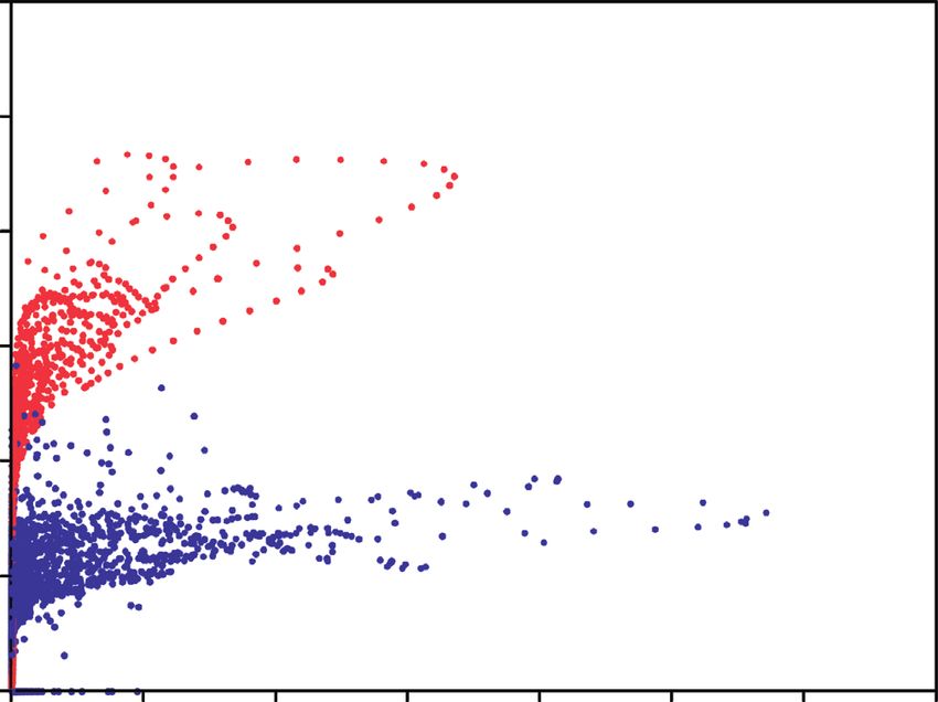
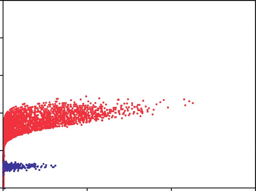
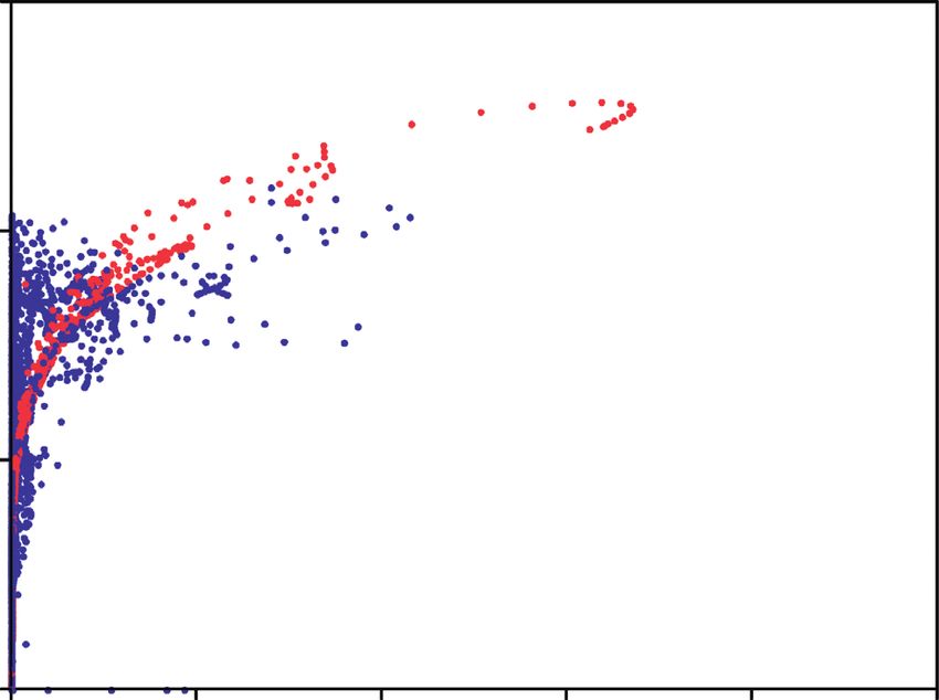
Advances in Meteorology 11

experiments underestimates the hourly precipitation RMSE. breakup occurs, the number of smaller raindrops increases,
A plausible cause is that terminal velocity perturbations are which decreases the mass-weighted terminal velocity so that
effective only in areas with nonzero hydrometeors, and the the amount of rainwater reaching the ground does not
difference among members was zero in the initial members increase as much as when using the Lin scheme. Further
to prevent the introduction of spurious precipitation [28]. investigation (not shown) indicates that more small rain-
Using a more advanced method to generate initial members drops appear when the precipitation area is collocated with
may increase the ensemble spread, although this is beyond perturbations greater than 1.0, supporting the above
the scope of the present work. In addition, the results in speculation.
Figure 6(a) also indicate that the MY2 scheme outperforms Although terminal velocity perturbations have positive
the Lin scheme even when the terminal velocity perturba- impacts on precipitation amount forecasts, the impact on
tions are applied to the Lin scheme. Although MY2prt_ref precipitation probability forecasts is not so clear. The reli-
requires much more computational resources than LINpr- ability results (Figures 6(e)–6(f )) indicate that all experi-
t_ref, a two-moment scheme is preferable when the com- ments overestimated the precipitation probability. There is
putational resources are sufficient. no significant difference between experiments with and
 The results of areal accumulated precipitation without terminal velocity perturbations. Further examina-
(Figure 6(b)) indicate that all experiments overestimated the tion (not shown) indicates that the overestimation is as-
precipitation amount in the verification domain, even when sociated with the fact that the predicted precipitation areas
the two-moment scheme was adopted. Despite the above in all experiments were larger than the observed precipi-
bias, the experiments with terminal velocity perturbations tation areas, consistent with the overprediction shown in
produced areal accumulated precipitation values closer to Figure 6(c).
the observation than the experiments with only initial Figure 7 shows an intuitive comparison of the best
conditions, especially in the last two hours. Further exam- members in LINens, MY2ens, LINprt_ref, and MY2prt_ref
ination (not shown) indicates that most members of with respect to the hourly precipitation RMSE. All of these
LINprt_ref and MY2prt_ref yielded lower areal accumulated members capture the observed precipitation band but differ
precipitation values than their counterparts in LINens and in detail. At 01 UTC, members of LINens and LINprt_ref
MY2ens, implying that the better forecasts of the areal ac- overpredicted the observed precipitation maximum, which
cumulated precipitation are unlikely to have occurred by is better matched by members of MY2ens and MY2prt_ref.
chance. This difference is consistent with Figure 6(b), in which the
 The bias scores (Figure 6(c)) demonstrate that all ex- observed areal accumulated precipitation is well matched
periments have small biases at the light rain (1 mm·h− 1) with MY2ens and MY2prt_ref. At 02 UTC, all members in
threshold but larger biases as the threshold increases. All Figure 7 overpredict the precipitation amount in north-
experiments overpredicted the precipitation events at eastern Alabama, which corresponds to the increased error
thresholds over 5 mm·h− 1, indicating that the areal accu- in all experiments in Figure 6. At 03 UTC, the observed
mulated precipitation errors are mainly attributable to the precipitation peak (>30 mm·h− 1) is approximately captured
biases associated with moderate and heavy rain. Even though by all members, where the LINens and LINprt_ref members
large biases exist, LINprt_ref and MY2prt_ref produced are intuitively better than the MY2ens and MY2prt_ref
smaller biases than LINens and MY2ens, except for light members in terms of the precipitation peak distribution. To
rain, indicating that perturbing the terminal velocity is likely the northeast of this observed maximum, a pronounced
to benefit the precipitation forecasts in real cases. The ex- overprediction occurs in LINens, while the overprediction
amination of precipitation frequencies (Figure 6(d)) further was alleviated in LINprt_ref, consistent with the results in
confirms the above improvement in precipitation amounts. Figures 6(b) and 6(c).
LINprt_ref produced a precipitation frequency comparable To determine the cause of the overprediction in
to that of MY2ens for precipitation rates lower than northwestern Georgia (along approximately 34.4°N) in
10 mm·h− 1, which can be partly explained by the pertur- LINens member 2, the vertical distributions of hydrome-
bation parameters in LINprt_ref being tuned according to teors and their terminal velocities are examined (Figure 8).
the difference between the Lin scheme and the MY2 scheme. Along 34.4°N, LINens member 2 has the smallest meridional
MY2prt_ref yielded a precipitation frequency closest to the average qh in the mid-levels. However, this member pro-
observation, and thus it has the smallest RMSE and pre- duces the largest falling speeds of both hail and rainwater
cipitation bias. among the examined members. Therefore, the overestimated
 The good performance of LINprt_ref is attributable to terminal velocities result in overpredicted precipitation in
the terminal velocity perturbations being systematically set LINens member 2. Otherwise, the smaller qh in this member
to values smaller than 1.0, but the reason for the good should have produced smaller precipitation amounts with
performance of MY2prt_ref is not that straightforward terminal velocities identical to that of LINprt_ref member 2.
because symmetric perturbations were used. Considering In addition, the rainwater terminal velocity in LINprt_ref
that the MY2 scheme allows a raindrop breakup effect, a member 2 is also smaller than that of MY2ens member 2 in
plausible explanation is that perturbation greater than 1.0 northwestern Georgia, which leads to the precipitation in-
increases not only the terminal velocities of hydrometeors tensity in LINprt_ref member 2 being closer to the obser-
but also the collisional kinetic energy (CKE), which increases vation. This situation is also valid for the comparison
the chance of raindrop breakup [43, 67]. As raindrop between MY2prt_ref and MY2ens. The above results imply

12 Advances in Meteorology

 (mm/h) (mm/h) (mm/h) (mm/h)

 30 30 30 30
 10 10 10 10
 Georgia Georgia Georgia Georgia
 1 10 1 10 1 10 1 10

 1 1 1 1
 Alabama Alabama Alabama Alabama
 LINens mem2 T = 01UTC MY2ens mem2 T = 01 UTC LINprt_ref mem2 T = 01 UTC MY2prt_ref mem2 T = 01UTC

 (a) (b) (c) (d)
 (mm/h) (mm/h) (mm/h) (mm/h)

 30 30 30 30

 10 10 10 10
 1 10 1 10 1 10 1 10

 1 1 1 1
 Alabama Alabama Alabama Alabama
 LINens mem2 T = 02UTC MY2ens mem2 T = 02 UTC LINprt_ref mem2 T = 02 UTC MY2prt_ref mem2 T = 02UTC

 (e) (f) (g) (h)
 (mm/h) (mm/h) (mm/h) (mm/h)

 35N
 30 30 30 30

 34N 10 10 10 10
 30 10 30 10 30 10 30 10
 1 1 1 1
 33N 1 1 1 1
 Alabama Alabama Alabama Alabama
 LINens mem2 T = 03UTC MY2ens mem2 T = 03 UTC LINprt_ref mem2 T = 03 UTC MY2prt_ref mem2 T = 03UTC

 88W 87W 86W 85W
 (i) (j) (k) (l)
Figure 7: Hourly precipitation rate from the observations (contour) and (a, e, i) LINens, (b, f, j) MY2ens, (c, g, k) LINprt_ref, and (d, h, l)
MY2prt_ref at 01 ZUTC (upper panels), 02 ZUTC (middle panels), and 03 ZUTC (lower panels).

that the terminal velocities yielded by a two-moment scheme The better precipitation amount forecast in LINpr-
are not necessarily perfect; thus, the stochastic perturbation t_ref_K corresponds to a smaller bias (Figure 9(c)) and a
approach applied to hydrometeor terminal velocities could precipitation frequency that is close to the observations;
aid in the skill of precipitation forecasting. However, no- an example at 03 UTC is shown in Figure 9(d). Unlike
tably, the overpredicted precipitation in MY2ens does not LINprt_ref_K, MY2prt_ref_K does not outperform
have to result from inaccurate terminal velocities; the MY2ens_K in terms of the precipitation error
contents of hail and rain may be overestimated, which can (Figure 9(a)) and the areal accumulated precipitation
also cause a large amount of precipitation. (Figure 9(b)). However, MY2prt_ref_K still produces a
 smaller bias than MY2ens_K, indicating that the impact of
 terminal velocity perturbations on the MY2 scheme is
4.2.2. Kansas Case. The benefits from stochastically per- similar in both cases, although the precipitation forecast
turbing the terminal velocities yielded by the Lin scheme are skill with the terminal velocity perturbations depends on
again found in the Kansas case in terms of the RMSE of the case. The reliabilities of the probability forecasts in the
hourly precipitation (Figure 9(a)) and the areal accumulated Kansas case (not shown) are low in all cases, indicating
precipitation (Figure 9(b)). Additionally, the ensemble again that terminal velocity perturbations mainly con-
spread is still insensitive to the terminal velocity perturba- tribute to improvements in the predicted precipitation
tions. In this case, the overprediction of areal accumulated amount. To determine the plausible causes of the con-
precipitation occurs in all experiments; thus, most members sistent outperformance of perturbing terminal velocities
in LINprt_ref_K, which allows a terminal velocity bias, in the Lin scheme and the case-dependent performance of
produce areal accumulated precipitation values that are close terminal velocity perturbations in the MY2 scheme, we
to the observations, compared to that of LINens_K. The qualitatively examined the precipitation structure in all
similar trends in the precipitation error and areal precipi- experiments for the Kansas case.
tation amount in LINprt_ref_K and LINens_K (Figure 9(a) For each ensemble, the member having the smallest
and 9(b)) imply that the smaller precipitation error is mainly precipitation RMSE in the ensemble at 03 UTC was selected
attributable to the better prediction of the areal precipitation for the qualitative analysis. In Figure 10, all precipitation
amount in LINprt_ref_K.

Advances in Meteorology 13

 13.45 13.45
 11.75 11.75
 10.19 10.19
 8.67 8.67
 Altitude (km)

 Altitude (km)
 7.17 7.17
 5.68 5.68
 4.20 4.20
 2.81 2.81
 1.57 1.57
 0.61 0.61
 0.08 LINens 0.08 LINprt_ref

 85.2°W 85.0°W 84.8°W 84.6°W 84.4°W 85.2°W 85.0°W 84.8°W 84.6°W 84.4°W

 qr qh tvs qr qh tvs
 qs tvr tvh qs tvr tvh

 (a) (b)
 13.45 13.45
 11.75 11.75
 MY2ens MY2prt_ref
 10.19 10.19
 8.67 8.67
 Altitude (km)

 Altitude (km)

 7.17 7.17
 5.68 5.68
 4.20 4.20
 2.81 2.81
 1.57 1.57
 0.61 0.61
 0.08 0.08

 85.2°W 85.0°W 84.8°W 84.6°W 84.4°W 85.2°W 85.0°W 84.8°W 84.6°W 84.4°W

 qr qh tvs qr qh tvs
 qs tvr tvh qs tvr tvh

 (c) (d)

Figure 8: Vertical cross-sections of qr (red solid, g·kg− 1), qs (green solid, g·kg− 1), qh (blue solid, g·kg− 1), and their corresponding terminal
velocities (dot-dashed, m·s− 1) at 0230 ZUTC along 34.4°N for (a) LINens, (b) LINprt_ref, (c) MY2ens, and (d) MY2prt_ref. Values shown in
this figure are the meridional averages between 34.2°N and 34.6°N.

forecasts capture the observed precipitation band oriented in Figure 9(d) that the precipitation frequency of LINprt_ref_K
the southwest-northeast direction at 01 UTC and two is closer to the observations than that of LINens_K for
precipitation peaks at 02 UTC and 03 UTC, but there is precipitation greater than 10 mm·h− 1. Since the Lin scheme
clearly displacement in all forecasts. Although the precipi- often overestimates precipitation due to the unrealistically
tation distributions of members in LINprt_ref_K and high terminal velocities, using stochastically perturbed but
LINens_K look similar, member 10 in LINprt_ref_K pro- systematically smaller terminal velocities often helps pre-
duces less spurious precipitation than member 9 in LIN- cipitation forecasts.
ens_K. Further examination (not shown) indicates that, in Although the MY2 scheme members look similar
member 10, negative perturbations (before resampling) throughout the forecast period, they differ in their details,
prevail in the third forecast hour in northeastern Kansas, especially at 03 UTC. At that time, the spurious precipitation
which results in lower terminal velocities in that area; thus, area is smaller in member 9 in MY2prt_ref_K than in
the spurious precipitation amount is smaller in the member 2 in MY2ens_K, which contributes to the smaller
LINprt_ref_K member than that in LINens_K. The heavy RMSE of the former than that of the latter (not shown).
rainfall areas (red areas in Figures 10(a), 10(c), 10(e), 10(g), However, this better forecast occurs only in a few members,
10(i), and 10(k)) are also intuitively smaller in the LINpr- as shown in Figure 9(a). In most members in MY2prt_ref_K,
t_ref_K member, which is consistent with the result in the spurious precipitation areas are slightly larger than those

14 Advances in Meteorology

 18 1.9

 Areal accumulated precipitation (mm/grid point)
 16

 14 1.5

 12
 RMSE (mm/h)

 1.1
 10

 8
 0.8
 6

 4 0.4
 2

 0 0
 0.5 1 1.5 2 2.5 3 3.5 1 2 3
 Model time (h) Model time (h)

 LINens_K LINens_K ST4 LINprt_ref_K
 MY2ens_K MY2ens_K LINens_K MY2prt_ref_K
 LINprt_ref_K LINprt_ref_K MY2ens_K
 MY2prt_ref_K MY2prt_ref_K
 (a) (b)

 Time = 3h
 0.20
 Precipitation frequency

 0.8
 0.15
 0.6

 0.10
 0.4
 Logarithmic bias

 0.2 0.05

 0 0.00
 1 5 10 20 30 2 4 6 8 10 12 14 16 18 20
 –0.2 Precipitation (mm/h)

 ST4 MY2ens_K
 –0.4 LINens_K MY2prt_ref_K
 Precipitation rate (mm/h) LINprt_ref_K

 LINens_K MY2ens_K
 LINprt_ref_K MY2prt_ref_K
 (c) (d)

 Figure 9: The same as in Figure 6, except for LINens_K, MY2ens_K, LINprt_ref, and MY2prt_ref_K.

in MY2ens_K at 03 UTC (not shown); this is the reason that experiments produce larger precipitation areas than the
the mean areal accumulated precipitation is slightly larger observations. Additionally, the observed precipitation
in MY2prt_ref_K than in MY2ens_K. Moreover, com- peaks at 02 UTC and 03 UTC (Figures 10(f ), 10(h), 10(j),
paring Figures 9(d) and 6(d), symmetrically perturbing the and 10(l)), especially for the south peak, are often
terminal velocities in the MY2 scheme tends to produce underestimated by the MY2 scheme members. This result
more light rain (

Advances in Meteorology 15

 (mm/h) (mm/h) (mm/h) (mm/h)

 10 30 10 30 10 30 10 30

 10 10 10 1 10
 1 1 1
 LINens_K mem9 MY2ens_K mem2 LINprt_ref_K mem10 MY2prt_ref_K mem9
 1 1 1 1
 Kansas Kansas Kansas Kansas
 T = 01 UTC 26 May 2012 T = 01UTC 26 May 2012 T = 01UTC 26 May 2012 T = 01 UTC 26 May 2012

 (a) (b) (c) (d)
 (mm/h) (mm/h) (mm/h) (mm/h)

 10 30 10 30 10 30 10 30
 10 10 10 10
 1 10 1 10 10 10
 1 1
 LINens_K mem9 MY2ens_K mem2 LINprt_ref_K mem10 MY2prt_ref_K mem9
 1 1 1 1
 Kansas Kansas Kansas Kansas
 T = 02UTC 26 May 2012 T = 02UTC 26 May 2012 T = 02UTC 26 May 2012 T = 02 UTC 26 May 2012

 (e) (f) (g) (h)
 (mm/h) (mm/h) (mm/h) (mm/h)

 39°W 10 30 10 30 10 30 10 30
 10 10 10 10
 1 10 1 10 1 10 1 10
 LINens_K mem9 MY2ens_Kmem2 LINprt_ref_K mem10 MY2prt_ref_K mem9
 38°W 1 1 Kansas 1 1
 Kansas Kansas Kansas
 T = 03 UTC 26 May 2012 T = 03UTC 26 May 2012 T = 03UTC 26 May 2012 T = 03 UTC 26 May 2012
 100°W 99°W 98°W
 (i) (j) (k) (l)
Figure 10: The same as in Figure 7, except for (a, e, i) LINens_K, (b, f, j) MY2ens_K, (c, g, k) LINprt_ref_K, and (d, h, l) MY2prt_ref_K.

5. Summary and Conclusions symmetric terminal velocity perturbations within ±25%
 reduces the precipitation error in the case when the MY2
The focus of this work was on the impact of stochastically scheme overestimates precipitation; this perturbation ap-
perturbing the terminal velocities of hydrometeors on proach is ineffective in cases when precipitation is
convective-scale ensemble forecasts of precipitation. An underpredicted.
idealized supercell case was first employed. With this case As a preliminary work on terminal velocity pertur-
and assuming that the MY2 scheme was the truth, the re- bations, the potential benefits of using this type of per-
lationship between the precipitation and terminal velocities turbation were demonstrated. However, the experimental
was investigated. After determining the perturbation am- designs and results have many limitations; thus, it is not
plitudes that minimized the terminal velocity difference possible to establish a ranking of the configurations in
between the Lin scheme and MY2 scheme, ensemble fore- terms of probabilistic forecast skill. First, two real cases
casts with stochastic perturbations of terminal velocities are insufficient to confirm that terminal velocity pertur-
were performed and evaluated. Finally, the forecast skills of bations can produce statistically significantly better per-
stochastically perturbing the terminal velocities were ex- formances than those without terminal velocity
amined for both the one-moment and two-moment schemes perturbations. Second, only a 3 h forecast was performed
with two real cases. due to the computational limitation. Although the 3 h
 In terms of the results in Section 4, several conclusions forecasts are sufficient for the scope of this work, the
were obtained: (i) compared to the MY2 scheme, the ter- corresponding results are insufficient for longer-term
minal velocities of snow and hail are approximately 3 times forecasts, especially long-lived precipitation event fore-
larger in the Lin scheme, which is an important source of the casts. Longer forecast duration has to be considered for
overestimated precipitation in the Lin scheme experiments; the comprehensive evaluation of the terminal velocity
(ii) for the Lin scheme, it is better to perturb the terminal perturbations. In addition, the error characteristics of
velocities using perturbations smaller than 1.0, but note that terminal velocities depend on many microphysical pa-
these error characteristics depend on other parameters, such rameters, such as the intercept parameter and hydro-
as the intercept parameters in the microphysics scheme; (iii) meteor density; thus, the terminal velocity error
the Lin scheme often overestimates precipitation due to characteristics obtained in this work may not be valid for
overestimating the terminal velocities; thus, symmetrically other one-moment schemes. Finally, initial perturbations
perturbing terminal velocities by 25% around their original have not been considered but are essential in studies
values cannot effectively reduce the precipitation error when examining improvements in the probabilistic skill of this
the Lin scheme is used; (iv) for the MY2 scheme, the use of terminal velocity perturbation scheme.