Bell-state tomography in a silicon many-electron artificial molecule
←
→
Page content transcription
If your browser does not render page correctly, please read the page content below

Bell-state tomography in a silicon many-electron artificial molecule
Ross C. C. Leon,1, ∗ Chih Hwan Yang,1 Jason C. C. Hwang,1, † Julien Camirand Lemyre,2
Tuomo Tanttu,1 Wei Huang,1 Jonathan Y. Huang,1 Fay E. Hudson,1 Kohei M. Itoh,3
Arne Laucht,1 Michel Pioro-Ladrière,2, 4 Andre Saraiva,1, ‡ and Andrew S. Dzurak1, §
1
School of Electrical Engineering and Telecommunications,
The University of New South Wales, Sydney, NSW 2052, Australia.
2
Institut Quantique et Département de Physique,
Université de Sherbrooke, Sherbrooke, Québec J1K 2R1, Canada
3
School of Fundamental Science and Technology, Keio University,
arXiv:2008.03968v1 [cond-mat.mes-hall] 10 Aug 2020
3-14-1 Hiyoshi, Kohokuku, Yokohama 223-8522, Japan.
4
Quantum Information Science Program, Canadian Institute for Advanced Research, Toronto, ON, M5G 1Z8, Canada
An error-corrected quantum processor will re- ploit here the operation of qubits in silicon metal-oxide-
quire millions of qubits [1], accentuating the ad- semiconductor (Si-MOS) quantum dots containing sev-
vantage of nanoscale devices with small foot- eral electrons that form closed shells, leaving a single va-
prints, such as silicon quantum dots [2]. How- lence electron in the outer shell [3]. The spin of a valence
ever, as for every device with nanoscale dimen- electron in a high-occupancy Si-MOS quantum dot was
sions, disorder at the atomic level is detrimen- previously shown to form a high-fidelity single qubit [3],
tal to qubit uniformity. Here we investigate at least in part due to the improved screening of disorder
two spin qubits confined in a silicon double- provided by the raised electron density. However, it was
quantum-dot artificial molecule. Each quantum not clear how well two-qubit logic could be performed us-
dot has a robust shell structure and, when op- ing such systems, because of the complex molecular states
erated at an occupancy of 5 or 13 electrons, present in a many-electron double quantum dot [5]. We
has single spin-½ valence electron in its p- or address this here using two multielectron qubits to oper-
d -orbital, respectively [3]. These higher elec- ate an isolated quantum processing unit [8, 9].
tron occupancies screen atomic-level disorder [3–
5]. The larger multielectron wavefunctions also
This demonstration is performed with the device struc-
enable significant overlap between neighbouring
ture depicted in Figure 1a, and investigated in previous
qubit electrons, while making space for an inter-
studies [3, 9]. Using the technique adopted from Ref. 9,
stitial exchange-gate electrode. We implement a
where the quantum dots are isolated from the electron
universal gate set using the magnetic field gradi-
reservoir, we load electrons into the two quantum dots
ent of a micromagnet for electrically-driven sin-
formed under gates G1 and G2 and separated by gate
gle qubit gates [6], and a gate-voltage-controlled
J. We monitor inter-dot charge transitions by measuring
inter-dot barrier to perform two-qubit gates by
the transconductance of a nearby single electron transis-
pulsed exchange coupling. We use this gate set
tor (SET). An on-chip cobalt micromagnet is fabricated
to demonstrate a Bell state preparation between
120 nm away from the quantum dots. This micromag-
multielectron qubits with fidelity 90.3 %, con-
net serves two purposes: to create an inhomogeneous
firmed by two-qubit state tomography using spin
magnetic field as well as an oscillatory electric field, for
parity measurements [7].
electrically-driven spin resonance (EDSR) [6, 10, 11].
Semiconductor nanodevices, especially those incorpo-
rating oxide insulating layers, suffer from variability due In order to achieve an isolated mode of operation, the
to various atomic-scale defects and morphological impre- quantum dots are initialised with a desired number of
cision. This disorder degrades spin qubit performance electrons using the reservoir under RG, then the tunnel
due to the sub-nanometre wave properties of single elec- rate between the quantum dot under G2 and the reser-
trons. The conflict between the benefits of densely pack- voir is made negligible by lowering the voltage applied
ing many quantum dots within a chip and the expo- to gate BG, such that the double quantum dot becomes
sure to disorder demands further research regarding im- isolated [9]. Figure 1c is a charge stability diagram with
proved systems for encoding solid-state qubits. We ex- vertical lines indicating inter-dot charge transition. For
the experiment discussed here, we load a total of 18 elec-
trons. Note that diagonal lines on the upper half of Fig-
∗
ure 1c (around VJ = 1.9 V) mark transitions in which the
r.leon@unsw.edu.au
† Current address: Research and Prototype Foundry, The Univer- J gate becomes too attractive for electrons, and instead
sity of Sydney, Sydney, NSW 2006, Australia. of forming a barrier it forms a quantum dot between G1
‡ a.saraiva@unsw.edu.au and G2 [9]. At very low voltages, the J gate creates a
§ a.dzurak@unsw.edu.au large barrier between the dots suppressing inter-dot tun-
2
a b d
200n
m G1 J G2 30nm
0
B
Co 50
0]
[11
∆fESR (MHz)
0
T
SE
-50
Q2 Q1
0.8 0.8
RG
Podd
-100 0.3 0.2 100
CB
G1 200
J G2 50
0
BG -200 ε (mV)
∆VJ (mV)
c 2.2
(18,0)
2.0
(0,18)
VJ (V)
(17,1)
1.8
(1,17)
(16,2)
ISET (pA)
(2,16)
(3,15)
-30 70
(4,14)
(5,13)
(6,12)
(8,10)
(10,8)
(12,6)
(13,5)
(14,4)
(15,3)
(7,11)
(11,7)
(9,9)
1.6
-1 0 1
Detuning, ε (V)
Figure 1 | Device overview and electron occupancy measurement. a, A 3D visualisation of the Si-MOS device
structure. A quantum dot is formed under gate G1 (blue) and G2 (red), with inter-dot tunnel rates controlled by J (green).
Gate RG enables connection to an n-doped reservoir to load/unload electrons to/from the quantum dot, with tunnel rates
controlled by BG. Gate CB serves as a confinement barrier in lateral direction. The cobalt structure at the top of the image
acts as both a micromagnet and electrode for EDSR control (dark green). b, Top: Cross-section diagram of panel (a) along the
[11̄0] crystallographic direction. Bottom: Schematic showing the number of electrons in each of the two quantum dots, aligning
with the metal gates in the panel above. The height of each electron represents its relative energy and the shell to which it
belongs. Yellow electrons form full shells and are inert, while the extra electron in each dot (blue and red) act as an effective
single spin qubit. c, Charge stability map of the double quantum dot at B0 = 0 T, showing the charge occupancies (N1 ,N2 ),
produced by plotting the lock-in signal from SET sensor ISET as a function of detuning ε and VJ . The detuning ε = VG1 − VG2
is referenced by ε = 0 V at the charge readout transition (12,6)⇐⇒(13,5). A square wave with peak-to-peak amplitude of 2 mV
and frequency 487 Hz is applied to G1 for lock-in excitation. Dynamic compensation is applied to the SET sensor to maintain
a high readout sensitivity. d, Resonance frequency of Q1 and Q2 as a function of ε and VJ with |↓↓⟩ initialisation. Color scale
represents the adiabatic inversion probability.
nelling. Once the tunnel rate becomes lesser than the in each quantum dot (d-shell and p-shell, respectively)
lock-in frequency (487 Hz), the transition lines fade, as while the electrons in the inner shells stay inert during
observed for VJ < 1.6 V. spin operations [3]. Evidence supporting the p- and d-
In a small two dimensional circular quantum dot, full shell structures is demonstrated in the Methods section.
shells are formed at 4 and 12 electrons [3, 12–14]. The The particular choice of a p- and a d-shell electron is ar-
fourfold degeneracy of the first shell has its origin in the bitrary, solely for a proof-of-principle. In an earlier study,
spin and valley degrees of freedom for silicon conduc- we demonstrated the suitability of these shell configura-
tion band electrons. The next shell is formed by two- tions for single qubit operation, but a systematic study of
dimensional p-like states, which means the px and py the optimal number of electrons for a two-qubit system
states are quasi-degenerate in the approximately circu- is out of the scope of our present work.
larly symmetric dot. This shell can fit a total of 8 elec- In general, EDSR control of qubits is heavily influ-
trons. We control the voltage detuning ε between gates enced by the details of the quantum dot confinement po-
G1 and G2 voltages such that there are 13 and 5 electrons tential [15]. We investigate these parameters performing
in Q1 and Q2 respectively, as shown in Figure 1b and c. an adiabatic inversion of the spins with a variable fre-
This means we have effectively a single valence electron quency microwave excitation, with an external magnetic
3

field B0 = 1 T. Firstly, the detuning ε is varied across the    controlling inter-dot interactions – by detuning the quan-
(12,6)-(13,5) transition over a period of 500 µs, such that     tum dot potentials [17, 18], as shown in Figure 2a; or by
a |↓↓⟩ spin state is initialised adiabatically. We note that    directly controlling the inter-dot barrier potential via an
(12,6) provides a good initialisation because it is a spin-0    exchange J gate [11, 19, 20], as in Figure 2b.
configuration, as confirmed by magnetospectroscopy (see            For each method, the exchange intensity is measured
supplemental material). Moreover, a large anticrossing          by comparing the precession frequency of one qubit (tar-
gap between this (12,6) singlet and the |↓↓⟩ state at (13,5)    get) depending on the state of the other qubit (control)
occupation is created by the difference in quantization         with a Ramsey interferometry protocol. Due to the large
axes between dots due to the micromagnet field gradient.        difference in Larmor frequencies between quantum dots,
We further improve the fidelity of this initialisation by si-   only the z components of the spins couple to each other,
multaneously lowering VJ , in order to enhance the energy       while the x and y components oscillate at different rates
gap between this target state and the (14,4) singlet. Sub-      for each qubit and their coupling is on average vanish-
sequently, a chirped pulse of microwave excitation with         ingly small [21, 22]. The measured oscillations shown
variable frequency adiabatically flips one of the spins into    in Figure 2c and d result from a combination of the ex-
an antiparallel configuration, creating either a |↓↑⟩ or a      change coupling and the Stark shift introduced by the
|↑↓⟩ state, if the frequency sweep matches the resonance        gate pulses, measured with regard to a reference fre-
frequency of the qubit. This spin flip is then read out by      quency fref which can be conveniently chosen to opti-
quickly changing ε back to a (12,6) ground state, which         mise the accuracy of our measurements (see supplemen-
will be blockaded by the Pauli principle unless the spin        tary material). The exchange coupling may be obtained
flip to the antiparallel configuration was successful.          by taking the difference between the resulting frequencies
   Figure 1d shows the nonlinear dependency of the qubit        for the two states of the control qubit Q2 |↓⟩ and |↑⟩.
resonance frequencies with electric potentials (Stark              Figure 2e and f show the extracted oscillation frequen-
shift). Moreover, the efficiency of the adiabatic inver-        cies as controlled by either the detuning ε or the exchange
sion of the spins depends on the intensity of the effective     gate voltage VJ . The difference in oscillation frequencies
oscillatory field that drives Rabi oscillations. This is in-    corresponds to the exchange coupling and can be tuned
dicated by the colours in Figure 1d, and shows that each        over two orders of magnitude, as seen in the extracted
qubit has a different optimal gate configuration, such that     exchange coupling intensities in Figure 2g and h.We use
a sufficiently fast Rabi oscillation frequency is obtained      this conditional control to implement the two-qubit CZ
to ensure good control fidelity. This dependence of the         gate. The impact of exchange coupling on qubit coher-
Rabi frequency on the gate voltage configurations was           ence is quantified by extracting the decay time of the ex-
observed previously, and associated with the electron po-       change oscillations T2CZ , shown in Figure 2i as a function
sition shifting under the micromagnet field [3]. For more       of the extracted exchange coupling for both CZ opera-
information on the method of choosing the optimal op-           tion methods. We observe an improvement in the driven
eration point, analysis of the Rabi efficiencies and coher-     coherence times when the exchange control is performed
ence times of the qubits, refer to supplementary material.      by pulsing the J gate to control the inter-dot barrier, as
   The geometry of the MOS device studied here is known         compared to the detuning method. Since both methods
to lead to single electron wavefunctions that extend lat-       can reach similar exchange frequencies, this results in an
erally approximately 10 nm [16], which is consistent with       improvement in the quality factor of the exchange oscilla-
the large charging energy previously measured in this de-       tions Q = J × T2CZ as seen in Figure 2j, similarly to pre-
vice when a second electron is added [3]. Since the nom-        viously reported experiments [20, 23]. Throughout the
inal distance from the centre of G1 to the centre of G2         rest of this work, we adopt the direct J gate-controlled
exceeds 60 nm, the inter-dot exchange coupling in the           exchange coupling method for the implementation of CZ
(1,1) charge configuration is predicted to be insufficient      logic gates.
for quantum operations – indeed, previous measurements             As shown in Figure 1d, both qubits possess a strongly
in the same device reveal that exchange is only observed        non-linear Stark shift and large variation in the efficiency
when the J gate is positive enough to form a dot under          of the EDSR drive. Single qubit control fidelity in excess
it [9]. At the p- and d-shells, nonetheless, the Coulomb        of 99 % was only achieved when the gate voltage configu-
repulsion from the core electrons leads to a larger wave-       ration was tuned differently for each qubit, as indicated
function for the valence electron. As a result, we are able     in the example gate sequence shown in Figure 3a. This
to measure a sizeable interaction between distant qubits.       leads to a major limitation – single qubit gates must
The ability to control the inter-dot interaction is crucial     be performed sequentially, while the other qubit is left
for high fidelity two qubit gate operations [11]. High fi-      idling [24], unable to be protected by refocusing tech-
delity single qubit gates require low exchange coupling         niques such as dynamical decoupling [17, 25] or pulse
to ensure individual addressibility, while two qubit gates      shaping [26]. Together with the two-qubit CZ gate, these
demand strong coupling for fast exchange oscillation with       gates span the two-qubit Clifford space (see Figure 3b for
minimal exposure to noise. We explore two methods for           illustration).
4
a VG1 VJ
VG2 e f b VG1 VJ
VG2
10
12
fCZ (MHz)
10
0
8
6 -10
g (I) (II) h (III) (IV)
ε 101 101
J (MHz)
c d
1 100 100 1
-1
0 10 10-1 0
10.5 + 1.2 = 8.8 + 0.9 =
(I) - = 100 110 120 -80 -40 0 40 (III) - =
10.5 + -1.6 = 0.4 + -1.5 =
1 Detuning, ε (mV) VJ (mV) 1
Podd (norm.)
Podd (norm.)
0 i 102 j 0
1 1
102
T2CZ ( s)
0
10.5 + 0.4 =
101 0
8.2 + 1.2 =
Q
(II) - = 1 (IV) - =
10.5 + -0.3 = 10 7.9 + 1.3 =
1 1
0
10
0 100 0
0 1 2 3 4 10-1 100 101 10-1 100 101 0 1 2 3 4
Exchange time, CZ ( s) Exchange time, CZ ( s)
J (MHz) J (MHz)
Figure 2 | Exchange control. a,b, Schematic showing the two different mechanisms to electrically control exchange coupling
between quantum dots, by (a) voltage detuning between G1 and G2 gate, and (b) barrier control with J gate. c,d, Examples
of CZ oscillations controlled via (c) detuning or (d) J gate. We apply a pulse sequence X1−CZ−X1, where X1 is a π2 rotation
around the x-axis of Q1, then measure the probability of an odd spin parity Podd . Green Roman numbers in each panel
correspond to the applied voltage indicated in (e-h), drawn as green dashed lines. Blue and red markers corresponds to
the normalised measured Podd with Q2 initialised as |↓⟩ or |↑⟩ respectively. The data is fitted using the equation Podd =
CZ
A
2
(1 − cos(2πfosc t)e−t/T2 ) + b. The Ramsey frequency fosc is displayed as blue or red text on the panel. In order to
compensate the strong Stark shift induced by gate pulsing, we adopt different rotating frames, offset by a reference frequency
fref between experiments, as presented in grey dashed curves behind each measurement data set. We extract the CZ frequency
fCZ = fref + fosc in a common frame and the difference between fCZ,Q2=|↓⟩ and fCZ,Q2=|↑⟩ , which gives the exchange coupling
frequency J, shown as black bold text. e,f, The oscillation frequency fCZ as a function of (e) detuning or (f ) J gate control.
Blue and red line corresponds to Q1 = |↓⟩ and |↑⟩, respectively. g,h, Extracted exchange oscillation frequency J. i, Damping
time T2CZ of the measured oscillations as a function of exchange coupling J, for Q2 = |↑⟩ and for detuning (yellow-green) and
J gate control (purple). j, Quality factor Q = J × T2CZ as a function of J, extracted from (i).
The strong Stark shift between operating points leads more precisely, the ZZ projection of the two qubits. In
to a phase accumulation with regard to a reference fre- order to read out other projections, single and two qubit
quency which must be accounted for in gate implementa- gate operations can be performed before readout. Fig-
tions (see supplementary material). In order to minimise ure 3c displays some key examples of such tomography
the gate error introduced by resonance frequency shifts protocols. The gate sequence illustrated in Figure 3b rep-
(due to electrical 1/f noise and 29 Si nuclear spin flips), a resents the example of an IZ measurement, which maps
number of feedback protocols are implemented. The fol- the spin state of the second qubit into the parities of
lowing input parameters are monitored periodically and the two-spin arrangement, regardless of the initial state
adjusted if necessary: SET bias voltage, readout voltage of the first spin. In order to completely reconstruct the
level, ESR frequencies of both qubits, phase accumula- 4 × 4 density matrix of a two qubit system, 15 linearly in-
tions at 5 different gate voltages for the logic gates, and dependent tomography projections are required [28] (the
exchange coupling. This results in a total of 10 feedback complete list is presented in the supplementary material).
calibrations in each experiment. Further information on The results for each Bell state are shown in Figure 3d-
phase and exchange coupling feedback is provided in the g. The state preparation fidelities range from 87.5 % to
supplementary section. 90.3 %, which compares favourably with state-of-the-art
We gauge the quality of our gate set implementation two spin qubit systems [8, 11, 29].
by preparing Bell states and evaluating them through Our study highlights various advantages of multielec-
two-qubit state tomography [27]. For a double quantum tron qubits which lead to efficient EDSR-based single
dot isolated from the reservoir, parity readout is used for qubit gates and extended reach of the exchange cou-
the measurements [9], which implies that a readout step pling between neighbouring qubits. The protocol for
will contain the collective information of both qubits, or logic gates developed here leads to promising fidelities5
a b X1 X1 X2 CZ X2 c Basis state Projection operations Outcome
2 qubits
100
P odd gate ZZ
0.7
VJ (mV)
0
0
X2
Q2 gates
-100 ZX
Q1 gates
-50 0 50 Q1 gates Q2 gates
fESR (MHz)
CZ X2
d e
Odd
IX
Even
Ph
2
as
e
0
0
1
X2 CZ X2
f g Amplitude
IZ
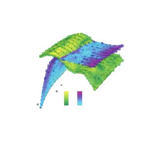
Figure 3 | Bell state tomography. a, Adiabatic inversion probability of both qubits as a function of detuned microwave
frequency, where the carrier frequency is chosen to be the single qubit operation frequency for Q2, and J gate voltage ∆VJ , with
qubits initialised in the |↓↓⟩ state. Horizontal dashed lines represent J gate voltages applied for various single qubit and two
qubit gates. Yellow dotted lines are a guide indicating the other resonance frequencies that would be observed at ∆VJ > 100 mV
if the spins were initialised randomly. b, Schematic of an example microwave and voltage pulse sequence for state tomography.
It initialises the qubits as |↑↓⟩ by performing two π2 X1 pulses (all calibration is performed for π2 pulses, such that a high fidelity
π pulse is obtained by composing it out of two π2 gates, each starting and finishing at a common voltage ∆VJ = −70 mV, which
is shown as a blue dashed line in (a)), then perform IZ projection operation, by converting the parity readout into single qubit
readout via a CNOT gate [9]. Horizontal lines align with ∆VJ from (a). c, Example qubit states and operations required to
obtain projections along the indicated axes. The first, two columns of Bloch spheres represent the eigenstates of Q1 (red) and
Q2 (blue) before state tomography, while the rest illustrates the logic gate operations required for state tomography, before
parity readout. For IX and IZ, all possible initial eigenstates are displayed, with parity results shown on the last column. d-g.
Quantum state tomography of Bell states (d) Φ+ = |↑↑⟩+|↓↓⟩√
2
, (e) Φ− = |↑↑⟩−|↓↓⟩
√
2
, (f ) Ψ+ = |↑↓⟩+|↓↑⟩
√
2
, (g) Ψ− = |↑↓⟩−|↓↑⟩
√
2
. The
height of the bars represents the absolute value of density matrix elements, while complex phase information is encoded in the
colour map. Inset: bar graph of the ideal density matrix of the corresponding Bell state. The measured fidelities of each Bell
state are (87.1 ± 2.8) %, (90.3 ± 3.0) %, (90.3 ± 2.4) % and (90.2 ± 2.9) %, from (d) to (g), respectively.
for Bell state preparation, but its use in longer compu- Si/SiO2 interface [4, 5], as demonstrated here, indicates
tations would be impacted by the inability to refocus that multielectron qubits offer a promising pathway for
the spin that is not being manipulated. This problem near term demonstrations of quantum processing in sili-
can be solved by designing a more efficient EDSR strat- con.
egy without the need to optimise the gate configuration,
or by using an antenna to produce microwave magnetic
field-based electron spin resonance [30]. The ability of
additional core electrons to screen charge disorder at the6
REFERENCES two individual electron spin qubits. Physical Review B
90, 075436 (2014).
[1] Campbell, E. T., Terhal, B. M. & Vuillot, C. Roads [23] Reed, M. et al. Reduced sensitivity to charge noise
towards fault-tolerant universal quantum computation. in semiconductor spin qubits via symmetric operation.
Nature 549, 172–179 (2017). Physical review letters 116, 110402 (2016).
[2] Zwanenburg, F. A. et al. Silicon quantum electronics. [24] Culcer, D., Hu, X. & Das Sarma, S. Dephasing of Si spin
Rev. Mod. Phys. 85, 961–1019 (2013). qubits due to charge noise. Applied Physics Letters 95,
[3] Leon, R. C. C. et al. Coherent spin control of s-, p- 073102 (2009).
, d- and f-electrons in a silicon quantum dot. Nature [25] Meiboom, S. & Gill, D. Modified spin-echo method for
Communications 11, 797 (2020). measuring nuclear relaxation times. Review of Scientific
[4] Barnes, E., Kestner, J. P., Nguyen, N. T. T. & Instruments 29, 688–691 (1958).
Das Sarma, S. Screening of charged impurities with [26] Yang, C. H. et al. Silicon qubit fidelities approaching in-
multielectron singlet-triplet spin qubits in quantum dots. coherent noise limits via pulse engineering. Nature Elec-
Physical Review B 84, 235309 (2011). tronics 2, 151–158 (2019).
[5] Hu, X. & Das Sarma, S. Spin-based quantum computa- [27] Man’ko, V. I. & Man’ko, O. V. Spin state tomogra-
tion in multielectron quantum dots. Physical Review A phy. Journal of Experimental and Theoretical Physics
64, 042312 (2001). 85, 430–434 (1997).
[6] Pioro-Ladrière, M. et al. Electrically driven single- [28] Rohling, N. & Burkard, G. Tomography scheme for two
electron spin resonance in a slanting zeeman field. Nature spin- 21 qubits in a double quantum dot. Physical Review
Physics 4, 776–779 (2008). B 88, 085402 (2013).
[7] Seedhouse, A. et al. Parity readout of silicon spin qubits [29] Huang, W. et al. Fidelity benchmarks for two-qubit gates
in quantum dots. arXiv:2004.07078 (2020). in silicon. Nature 569, 532–536 (2019).
[8] Watson, T. F. et al. A programmable two-qubit quantum [30] Veldhorst, M. et al. An addressable quantum dot qubit
processor in silicon. Nature 555, 633–637 (2018). with fault-tolerant control-fidelity. Nature Nanotechnol-
[9] Yang, C. H. et al. Operation of a silicon quantum pro- ogy 9, 981–985 (2014).
cessor unit cell above one kelvin. Nature 580, 350–354 [31] Laucht, A. et al. High-fidelity adiabatic inversion of a
(2020).
31
P electron spin qubit in natural silicon. Applied Physics
[10] Takeda, K. et al. A fault-tolerant addressable spin qubit Letters 104, 092115 (2014).
in a natural silicon quantum dot. Science Advances 2,
e1600694 (2016).
[11] Zajac, D. M. et al. Resonantly driven CNOT gate for
electron spins. Science 359, 439–442 (2018).
[12] Yang, C. H. et al. Spin-valley lifetimes in a silicon quan-
tum dot with tunable valley splitting. Nature Commu-
nications 4, 2069 (2013).
[13] Camenzind, L. C. et al. Spectroscopy of Quantum Dot
Orbitals with In-Plane Magnetic Fields. Physical Review
Letters 122, 207701 (2019).
[14] Liles, S. D. et al. Spin and orbital structure of the first
six holes in a silicon metal-oxide-semiconductor quantum
dot. Nature Communications 9, 3255 (2018).
[15] Camenzind, L. C. et al. Spectroscopy of quantum dot
orbitals with in-plane magnetic fields. Physical Review
Letters 122, 207701 (2019).
[16] Hensen, B. et al. A silicon quantum-dot-coupled nuclear
spin qubit. Nature Nanotechnology 15, 13–17 (2020).
[17] Petta, J. R. et al. Coherent manipulation of coupled
electron spins in semiconductor quantum dots. Science
309, 2180–2184 (2005).
[18] Veldhorst, M. et al. A two-qubit logic gate in silicon.
Nature 526, 410–414 (2015).
[19] Loss, D. & DiVincenzo, D. P. Quantum computation
with quantum dots. Physical Review A 57, 120–126
(1998).
[20] Martins, F. et al. Noise suppression using symmetric
exchange gates in spin qubits. Physical Review Letters
116, 116801 (2016).
[21] Meunier, T., Calado, V. & Vandersypen, L. Efficient
controlled-phase gate for single-spin qubits in quantum
dots. Physical Review B 83, 121403 (2011).
[22] Thalineau, R., Valentin, S. R., Wieck, A. D., Bäuerle, C.
& Meunier, T. Interplay between exchange interaction
and magnetic field gradient in a double quantum dot with7
METHODS This permits us to determine the resonance frequencies,
as well as the region of high qubit fidelity, as a function
Magnetospectroscopy of an isolated double quantum of detuning and J gate voltage.
dot
The colour scale in Figure 1d shows the extracted adia-
From the single dot shell structure [3], one can try to batic inversion probability of each qubit at various detun-
predict which double dot occupations will lead to a single ing and J gate voltages. We interpolated these probabil-
spin ½ qubit in each dot. But in order to confirm that ities and plotted them again in Extended Data Figure 2a
the spin structure of the double dot can be extrapolated and b. At first glance, we notice that Podd is symmetric
from single dot results, we obtain the spin ordering of along the axis of detuning ε = 37 mV, implying that de-
the dots performing magnetospectroscopy. Traditionally, tuning the dots in either direction has the same effect on
magnetospectroscopy is performed studying the shifts of dot shape and spin behaviour.
chemical potentials of each dot as a function of the ex-
ternally applied magnetic field. This assumes that the
The strategy to quickly calibrate the ideal operation
quantum dot is in diffusive equilibrium with a reservoir
points is to choose a few potential operation points on
(same chemical potential). Such reservoir is assumed to
the 2D map where Podd shows a high adiabatic inversion
be spinless, such that its chemical potential does not shift
probability, and measure the Rabi oscillation frequency
with magnetic field and the absolute shift in dot chemical
at a fixed microwave power. We then choose the highest
potential with magnetic field can be assessed. In our sys-
Rabi frequency point that meets some constrains. Firstly,
tem, the two dots are in equilibrium with each other, but
for individual addressability by frequency modulation,
all transitions conserve the total number of electrons in
the ESR frequency fESR of both qubits should be at least
the double dot system (isolated double dot) – there is no
10 MHz apart, which means ∆VJ < 20 mV or > 100 mV
reference reservoir, as shown in Extended Data Figure 1a.
in Figure 3a. Also, we would like to minimise the ex-
Therefore, only relative Zeeman shifts are observed.
change coupling during single qubit operation, which is
The hypothetical field dependencies, assuming that the
achieved for ∆VJ < −20 mV, setting J < 1 MHz as ob-
shell structure from Ref. 3 holds, are shown in the en-
served from Figure 2h. As a result, we are generally
ergy diagram in Extended Data Figure 1b. The measured
limited to the bottom half of the 2D map in Extended
magnetospectroscopy results in Extended Data Figure 1c
Data Figure 2a and b. Ideally, we would like to choose an
confirm our assumption. In particular, the (13,5) charge
optimal operation point such that we can perform single
configuration consists indeed of single spin-½ states in
qubit operation on both Q1 and Q2 (see main text for
both dots, each atop an inert closed shell of spin 0.
detail). However, there is no observable voltage range
Note that the leverarm we extracted from the slope in
from Extended Data Figure 2a and b where both qubits
Extended Data Figure 1c is the sum of leverarm from
gives high Podd under the constrains mentioned above.
Q1 and Q2, approximately αQ1 + αQ2 = 0.53 eV/V. Dif-
ferences in leverarm αQ1 − αQ2 cannot be obtained from
this method. A few detuning and J gate voltage combinations with
Podd > 0.42 are chosen for each qubit, and Rabi fre-
quencies are extracted in Extended Data Figure 2c and
Adiabatic inversion and qubit operation points d. The green markers from the plots are the opera-
tion points chosen for single qubit randomised bench-
In order to achieve single qubit EDSR control fidelities marking, with results presented in Extended Data Fig-
exceeding 99 %, compliant with the demands for quan- ure 2e and f. Qubits Q1 and Q2 have control fidelities
tum error correction in the surface code architecture, we FQ1 = (99.40 ± 0.17) % and FQ2 = (99.70 ± 0.10) %, re-
must adjust the inter-dot detuning and J gate voltage spectively. Note that the operation point chosen for Q2 is
such that we achieve the most efficient Rabi drive for not the one with the absolute maximum Rabi frequency,
both Q1 and Q2. as we also would like to minimise gate voltage fluctuation
We perform an adiabatic spin inversion experiment by when ramping between Q1 and Q2 logic gate operations.
sweeping the microwave frequency applied to the EDSR We observe a significant influence of ramping range on
gate electrode (in our case the Co magnet) at fixed power, the final outcome of the Bell state preparation, but a
such that when each of the qubit resonance frequencies thorough evaluation of this source of error is not war-
fESR is found, that spin is flipped with an efficiency given ranted, since this relates to instrument limitations.
by the comparison between the sweeping speed and the
Rabi frequency (limited by the spin relaxation time) [31]. Coherence times T2∗ for Q1 and Q2 at the chosen
This is observed as an increase in the probability of mea- operation points are (13.7 ± 2.0) µs and (8.4 ± 3.3) µs,
suring an odd parity readout after preparing the even respectively, while T2Hahn are (50.0 ± 15.2) µs and
initial state |↓↓⟩, with an example shown in Figure 3a. (94.6 ± 18.7) µs, respectively.8
a b c 0.2
0
(15,3)
(11,7) (12,6) (13,5) (14,4) -0.2
EQ1-EQ2 (meV)
(14,4)
0.2
EQ1-EQ2
0
(13,5)
(12,6) (13,5) (14,4) (15,3) 0
-0.2
(12,6)
-0.4
0 1 2 3 4
(11,7) B0 (T)
B0
Extended Data Figure 1 | Magnetospectroscopy of an isolated double quantum dot. a, Estimated spin state of
the active valence electrons before (top row of schematics) and after (bottom row of schematics) an inter-dot charge transition
at corresponding electron number (m,n), where m and n represent the total number of electrons in Q1 and Q2 respectively.
Coloured arrows represents the electron which participates in charge transition, with blue and red indicate spin down and up,
respectively. b, Illustration of energy difference between Q1 and Q2 as a function of applied magnetic field B0 , as corresponding
electron numbers in each dot. c, Extracted experimental magnetospectroscopy data, with each colour corresponding to the
energy difference in charge transition shown in (b).
Exchange oscillation, coherence and Q factors of termine the sign of ESR frequency shift, we repeat every
interacting spins Ramsey experiment with additional phase shift on the
second π2 pulse, in order to extract X,−X,Y,−Y projec-
The oscillations observed from Ramsey-like experi- tions of the qubit. Note that all four measurements are
ments in the main text Figure 2c, d are due to difference taken in a interleaved fashion to minimise the impact of
in precession frequency of the qubits in the period be- quasi-static noise.
tween π2 -pulses. The difference in frequencies arises from
both Stark shift, which is in the order of 10 MHz in our Measurement feedback
experiments, and exchange coupling J, between 100 kHz
and 10 MHz. As a result, the total Ramsey frequency
Low frequency noise is a major limitation for high fi-
will be dominated by Stark shift, making the J-coupling
delity operation of qubits in MOS devices [29]. An ef-
effect difficult to observe without a high resolution scan
ficient approach to mitigate high amplitude noise that
of precession time. Therefore, we adjust the phase of the
occurs in a sub-Hz scale is to recalibrate the most criti-
second π2 -pulse to match a rotating frame of reference
cal qubit control parameters periodically.
which is not the same as the qubit Q1 precession fre-
There are 10 parameters that require feedback
quency fQ1 , but instead it is offset by a value fref chosen
throughout the experiments due to the intricate way by
to reduce the impact of the Stark shift to the oscillation
which the qubit operations are defined with different gate
observed in experiment. This reference frequency is ad-
configurations targeting the optimisation of each qubit.
justed ad hoc between different experiments in order to
These parameters are the SET Coulomb peak alignment,
facilitate the extraction of the exchange coupling effect.
the readout level set by the dot gate, both qubit ESR
In the left panel of Figure 2, where the quantum dots frequencies, a total of five relative phases acquired when
are detuned, fref is set to 10.5 MHz throughout the ex- pulsing between operating points, and the exchange cou-
periment. However, for direct J gate controlled CZ, the pling controlled by the J gate. The SET feedback is used
oscillation frequency varies across a range of 20 MHz, as to maintain its high sensitivity during charge transition,
shown in Figure 2f. In order to capture the oscillation while read level feedback is to ensure the readout is done
data efficiently, we assign various fref for each ∆VJ tar- within a Pauli spin blockade region for parity readout.
geting a shift of approximately −1 MHz from the CZ fre- SET and readout level feedbacks are performed with first
quency fCZ (which could differ depending on whether the order corrections, with a predefined target SET current.
control spin is up or down). SET top gate voltage VST and read level voltage (con-
In a qubit rotating frame, positive and negative phase trolled via VG1 ) are updated based upon the difference
accumulation will result in the same Ramsey oscillation between measured current and target current.
if only a single measurement projection is taken. To de- We adopt the ESR frequency tracking protocol from9
a Q1 b Q2
150 150
100 100
50 50
VJ (mV)
VJ (mV)
0 0
-50 -50
Podd Podd
-100 0.8
-100 0.8
0.3
-150 -150 0.3
20 30 40 50 20 30 40 50
Detuning, ε (mV) Detuning, ε (mV)
c d
Detuning, ε (mV) Detuning, ε (mV)
e 1.2 f 1
Fele = 99.4% Fele = 99.7%
1
Podd (norm.)
Podd (norm.)
0.8
0.8
0.6
0.6
0.4 0.4
0 100 200 300 0 100 200 300
Number of Clifford gates (L) Number of Clifford gates (L)
Extended Data Figure 2 | Single qubit operation voltage. a,b, Adiabatic inversion probability of (a) Q1 or (a) Q2
as a function of detuning and J gate voltage, with interpolation. c,d, Rabi frequency fRabi for selected detuning and J gate
voltage combinations, with the 2D plot of panels (a) and (b) copied at bottom of x-y plane. e,f, Single qubit randomised
benchmarking for (e) Q1 or (f ) Q2 at voltages at the green marker in panels (c) and (d), respectively.10
Ref. 29 in order to follow the resonance frequency jumps Exchange coupling feedback
due to quasi-static noise such as hyperfine coupling with
residual 29 Si nuclear spin in the silicon wafer, as well The exchange coupling J may fluctuate between ex-
as low frequency electrical noise. We perform checks of periments due to low frequency electrical noise, which
each of the two resonance frequencies shown in Figure 3a can be compensated by monitoring and recalibrating the
independently every 10 measurement data points. If the CZ gate operation with a feedback protocol. The sam-
spin rotation is unsuccessful at the assumed resonance pling rate of the arbitrary waveform generator (AWG)
frequency, we recalibrate the frequency with a series of and microwave IQ modulation used here, 8 ns and 10 ns
Ramsey experiments. respectively, limit our gate operation times to the least
In Figure 3a, the ESR frequency shift ∆fESR is common multiple of these two, τCZ = 40 ns, or any multi-
taken as 0 MHz at the microwave driving frequency that ples of that. This means that updating the CZ exchange
matches the resonance frequency of Q2 at voltage ∆VJ = time τCZ is not accurate enough for high fidelity opera-
−70 mV, which is the operating point for Q2. At all the tion. Instead, we update the inter-dot barrier gate volt-
other operation points where ∆fESR is non-zero, a phase age VJ , which compensates the change in J while leaving
will accumulate due to variations in precession frequency. τCZ unchanged.
Since our Clifford set requires 3 operation voltages, each The initial calibration method is as follows: two CZ
with two phases for Q1 and Q2 to track, excluding the identical sequences are performed, each one with an op-
reference frequency fESR = fQ2 , that results in 5 phase posite control qubit state (spin down or up). We vary
accumulations to recalibrate. the readout projection angles ϕ and fit the parity read-
out probability to a sinusoidal wave similar to the case
Although phase accumulation can be calculated by the of the phase feedback, which we use to extract the phase
extracted ESR frequency (∆fESR ) and gate time tg , i.e. offset ϕ′fit . The difference in phase accumulated in the
ϕ = ∆fESR × tg , such method assumes an instantaneous control spin down and up cases are due to the composi-
step from one gate voltage to another, which in reality is tion of an exchange coupling from the CZ operation and
limited by the 80 MHz bandwidth of the measurement from the extra X22 gate necessary for the control spin
cable, meaning during the ramp both qubits spend a up calibration step. The latter can be compensated by
non-negligible amount of time in an intermediate voltage re-scaling ϕ′fit to 0 at low exchange coupling regime.
state, accumulating phases that are non-trivial to calcu-
This experiment is repeated with various exchange
late, especially when the Stark shift is highly non-linear
gate voltages ∆VJ , as shown in Extended Data Figure 3a
as seen in Figure 3a. Moreover, it is unclear whether the
and b, while the resulting phases, are plotted on Ex-
low frequency noise will affect the overall shape of the
tended Data Figure 3c, along with an exponential fit.
gate dependency of the resonant frequencies.
The difference between the two lines in Extended Data
In quantum computing, all operations can be per- Figure 3c are the phase contributed from exchange cou-
δϕ′fit
formed by a sequence of gates taken from a primitive pling J, which can be calculated from J = τCZ .
gate set. The processing unit is fully calibrated if all Upon choosing the desired value of J with the associ-
the primitive gates are calibrated individually. Table I ated ∆VJ , which should correspond to a δϕ′fit = π phase
shows the pulse sequences required to extract each of the difference between the two initial states, a feedback pro-
5 phases accumulated, each associate with certain qubit tocol can be implemented to recalibrate J periodically.
and primitive gates. The feedback protocol is similar to the initial calibration
Phase calibration is performed every ten measure- mentioned above, but optimised for speed by focusing on
ments, after the ESR frequencies are updated. In each a smaller range of ∆VJ , and the exponential fit used in
calibration, the corresponding pulse sequence from Ta- Extended Data Figure 3c is replaced with a linear fit.
ble I is applied with various phases ϕ for the last π2 pulse With that, the value of ∆VJ is updated using the fit in
with respect to the other pulses. The results are then fit- order to maintain the same exchange coupling strength
ted with a function Podd = A cos(2π(ϕ − ϕ′ )) + b, where J.
A and b are fitting constants related to the oscillation This exchange coupling feedback is performed after ten
visibility and dark counts, while ϕ′ is the phase accumu- measurements, immediately after the phase calibration
lated from the target gate. Since this protocol may rely step. Note that the pulse sequence used in Extended
on multiple primitive gates in a sequence, the phase as- Data Figure 3a is identical to the one in Table I. There-
sociated with each gate in Table I has to be calibrated fore, the X1−CZ−X1 sequence is omitted from the phase
following a certain order , to ensure the phase extracted calibration stage, but extracted from the subsequent ex-
corresponds to one particular primitive gate only. These change coupling feedback stage.
phases ϕ′ will be used for compensation of unwanted ac- Extended Data Figure 4 is an example of a Bell state
cumulated phases as we apply the corresponding Clifford tomography experiment, with all ten feedback loops ac-
gates in the experiment. tive, and the variation of the respective parameters over11
Level ∆VJ (mV) Q1 target gate Q2 target gate Primitive gate
1 -120 X12 I1 X2−I1−X2 I1 X1,Y1
2 -70 X1−I2−X1 I2 N/A N/A X2,Y2
3 130 X1−CZ−X1 CZ X2−CZ−X2 CZ CZ
Table I | Pulse sequences for qubit phase calibration. Pulse sequences used to extract phase accumulation while idling.
∆VJ (mV) is referenced from Figure 3a. Element at column Qn row ∆VJ corresponds to pulse sequence required to extract
phase accumulated in qubit n when inter-dot barrier gate voltage is at ∆VJ . Rn represents a π2 rotation around R-axis on qubit
n, with R ∈ {X, Y}, while In means identity gate with ∆VJ equals to the voltage where single qubit operation is performed for
qubit n.
a b c
130
120 fit
VJ (mV)
110
100
Peven Podd
90 0.8 0.8
0.1 0.1
80
- 0 - 0 - 0
Phase offset Phase offset Relative phase fit
Extended Data Figure 3 | Phase accumulation from CZ operation. a,b, Parity readout probability as a func-
tion of exchange gate voltage ∆VJ and phase offset ϕ, for duration of τCZ = 160 ns, with gates (a) X1−CZ−X1(ϕ) or (b)
X22 −X1−CZ−X1(ϕ) applied. ϕ represent the phase offset of the second X1 pulse with respect to the first within the same
sequence. Marker in each row indicate the fitted phase ϕ′ from a Peven/odd = A cos(2π(ϕ − ϕ′ )) + b, where A,b and ϕ′ are
constants. Note that since the control qubit is initilised into opposite spin state and parity readout is used, opposite parity is
extracted for the two cases in order to obtain the same single spin information from the target qubit. c, Fitted phase ϕ′ from
(a) (green ‘×’) and (b) (red ‘+’), which are fitted with equation ϕ′fit = A exp(−b∆VJ ) + c, where A, b and c are constants.
Both graphs are offset to zero phase at ∆VJ = 80 mV.
40 minutes of laboratory time. The parameters that are odd parity probability Podd corresponding to the 15 pro-
calibrated only every ten measurements have larger gaps jections from Table II.
between data points. Firstly, we factor in the errors associated with state
initialisation and measurement (SPAM error), by renor-
malising the parity readout probability of the two qubits
Two qubit tomography with parity readout for ZZ readout.
Next, we reconstruct the density matrix from the mea-
A two qubit density matrix is a 4 × 4 matrix spanning surement data. Let Eυ be the measurement outcome pro-
a 42 − 1 = 15 dimensional space and requires 15 lin- jector, ρ be density matrix, pυ be the measurement prob-
early independent projection measurements. Ref. 7 gives ability, where υ = 1...30 (notice that measurements of the
a detailed explanation on how to perform two-qubit state projector PM N , where M, N ∈ {I, X, Y, Z}, produce not
tomography using parity readout. Table II lists the gate only probability pM N , but also p−M N = 1 − pM N , so
operation sequences adopted here for each of the 15 pro- that 15 projections yield 30 probabilities). We define a
jection measurements, using a combination of primitive matrix A as
gates described in the main text. ⃗†
E1
E⃗†
2
A= . (1)
Fidelity estimation ..
⃗† ,
E 30
In order to accurately estimate the fidelity of the con-
trol steps in preparing a Bell state, some post-processing where E
⃗ υ† stands for the vectorised form of the projection
techniques are applied to the outcome of the measured Eυ .12
a
VST (mV)
-27.8
-28
b -2.6
voltage (mV)
Read level
-2.8
c
frequency (kHz)
100
ESR
50
0
d
/2
11
0 12
Phase
13
21
- /2 23
e
126
VJ (mV)
125
124
0 10 20 30 40
Time (mins)
Extended Data Figure 4 | Parameters tracking over measurement time. Various parameters are recorded while
Bell state tomography of Figure 3g is running. a, ST gate voltage ∆VST from SET feedback. b, G1 gate voltage ∆VG1
during readout, from parity readout feedback. c, Change in resonance frequency ∆ESR for Q1 (blue) and Q2 (red). d, Phase
accumulation ϕM N from the target gate in Table I, where M and N represents the level and qubit in the table, respectively.
e, J gate voltage ∆VJ required to maintain a phase difference of δϕ′fit = π at τCZ = 160 ns during CZ operation.13
Projection Operations and t1 ..t16 are real numbers. To find these values, we
ZZ I apply a maximum likelihood estimation, with the cost
YZ X1 function
XZ Y1
ZY X2 X (⟨ψυ |ρ̂(t1 , t2 , ...t16 )|ψυ ⟩ − nυ )2
ZX Y2 L(t1 , t2 , ...t16 ) = (5)
YY X1−X2 υ
2 ⟨ψυ |ρ̂(t1 , t2 , ...t16 )|ψυ ⟩
YX X1−Y2
XY Y1−X2 where ψυ is the vectorised measurement matrix with
XX Y1−Y2
υ = 1...30 and nυ are the measurement probabilities.
YI CZ−X1
XI CZ−Y1
We start our search inputing the density matrix result-
IY CZ−X2 ing from the pseudo-linear inversion described before
IX CZ−Y2 and proceed to numerically optimise L as a function of
ZI X1−CZ−X1 t1 , t2 , ...t16 . The resulting elements will give our final
IZ X2−CZ−X2 density matrix.
The fidelity of a Bell state
p√ is√calculated then from the
Table II | Gate operations for parity readout. List
definition F (ρ, ρ̂) = (tr{ ρρ̂ ρ})2 , where ρ and ρ̂ are
of operations required for a complete state tomography via
parity readout, with each row representing the projection axis the ideal and measured density matrices, respectively.
of interest for a two-qubit system, and the sequence of gate
operations required prior to readout.
DATA AVAILABILITY
Similarly, all elements of ρ can also be vectorised. This
yields the relation: The data that support the findings of this study are
⃗†
E1 ρ ⃗ tr{E1† ρ}
available from the authors on reasonable request, see au-
P (E1 |ρ)
E ⃗ † ⃗ tr{E † ρ} P (E2 |ρ) thor contributions for specific data sets.
2ρ 2
ρ= . =
A⃗ .. = ..
.. .
.
†
⃗ ρ † P (E30 |ρ)
E 30 ⃗ tr{E30 ρ}
(2) CODE AVAILABILITY
p1
p2
≈ . = p⃗
The code that support the findings of this study are
.. available from the authors on reasonable request, see au-
p30 thor contributions for specific code sets.
With matrix A constructed from our choice of measure-
ment projection, and p⃗ from measurement data. We then
perform a (pseudo) linear inversion to estimate the den- REFERENCES
sity matrix ρ̂.
Since the matrix computed numerically by linear in- ACKNOWLEDGMENTS
version can be an unphysical state for a qubit (leading to
a measured matrix p⃗ that does not have the properties
of a density matrix), a maximum likelihood technique is We acknowledge support from the Australian Research
used to numerically estimate the density matrix [? ] un- Council (FL190100167 and CE170100012), the US Army
der several constrains. A legitimate qubit density matrix Research Office (W911NF-17-1-0198), Silicon Quantum
must be non-negative definite, have a trace of one and Computing Pty Ltd, and the NSW Node of the Aus-
be Hermitian. These conditions are met if we write the tralian National Fabrication Facility. The views and
density matrix as [? ]: conclusions contained in this document are those of the
authors and should not be interpreted as representing
T †T the official policies, either expressed or implied, of the
ρ̂ = (3)
tr{T † T } Army Research Office or the U.S. Government. The U.S.
Government is authorized to reproduce and distribute
where
reprints for Government purposes notwithstanding any
copyright notation herein. J. C. and M. P. acknowledge
t1 0 0 0
t5 + it6 t 0 0 support from the Canada First Research Excellence Fund
T = 2
(4)
and in part by the National Science Engineering Research
t11 + it12 t7 + it8 t3 0
t15 + it16 t13 + it14 t9 + it10 t4 Council of Canada.14
AUTHOR CONTRIBUTIONS to the preparation of experiments. R.C.C.L., C.H.Y.,
A.S. and A.S.D. designed the experiments, with J.C.L.,
R.C.C.L. and C.H.Y. performed the experiments. M.P.-L., W.H., T.T., A.M. and A.L. contributing to
J.C.L., R.C.C.L., J.C.C.H., C.H.Y. and M.P.-L. designed results discussion and interpretation. R.C.C.L., A.S.,
the micromagnet, which was then simulated by J.C.L and A.S.D. wrote the manuscript with input from all
and M.P.-L. J.C.C.H. and F.E.H. fabricated the device co-authors. R.C.C.L. and J.Y.H. contributed in device
with A.S.D’s supervision. K.M.I. prepared and supplied visualisation in the manuscript.
the 28 Si epilayer. J.C.C.H., W.H. and T.T. contributedYou can also read