Poverty profile: rural North and Northeast of Brazil - IFAD Strategy for Brazil 2016-2021 and Series of Studies on Rural Poverty - FIDA
←
→
Page content transcription
If your browser does not render page correctly, please read the page content below
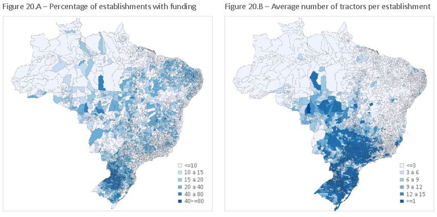
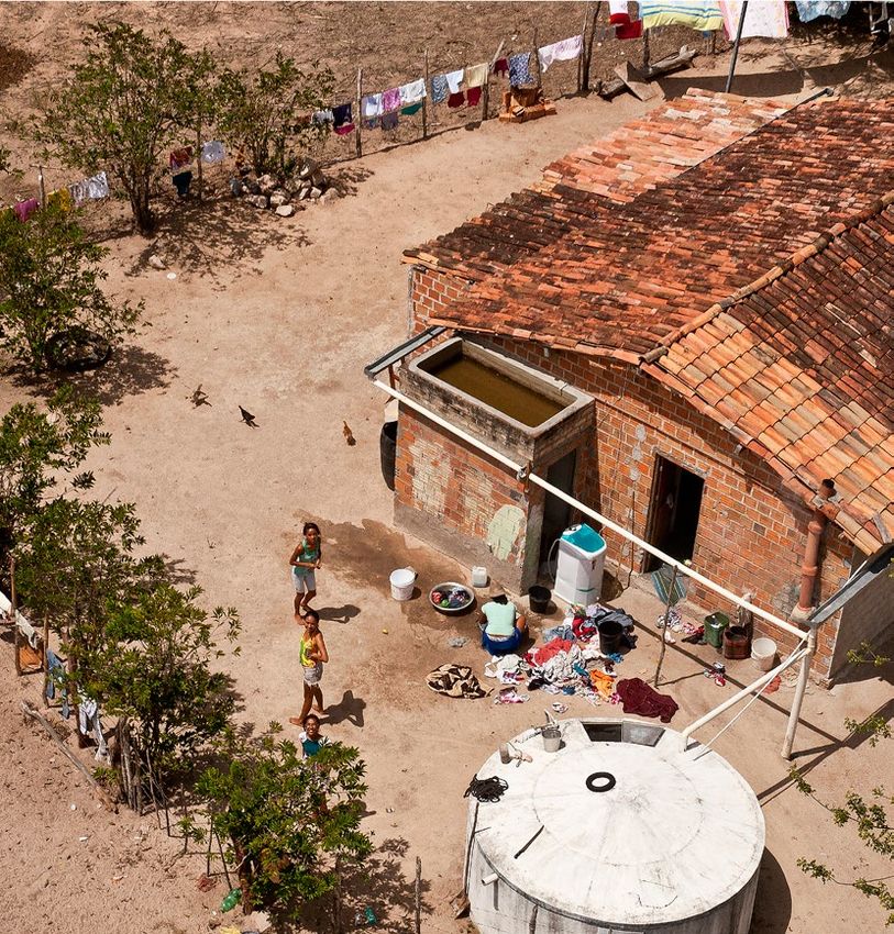
Photo: Sergio Amaral/MDS

 Poverty profile:
 rural North and Northeast of Brazil

 Investing in rural people

 IFAD Strategy for Brazil 2016-2021 and Series of Studies on Rural Poverty
Poverty profile: the rural North and Northeast of Brazil
Sergei Soares; Laetícia De Souza; Wesley Silva; Fernando Gaiger Silveira and Áquila Campos

This publication is a result of a partnership between the International Policy Centre for Inclusive Growth (IPC-IG),
the United Nations Development Programme (UNDP), the Institute for Applied Economic Research (Ipea)
and the International Fund for Agricultural Development (IFAD).

Copyright© 2016
International Policy Centre for Inclusive Growth
United Nations Development Programme

International Policy Centre for Inclusive Growth (IPC - IG)
United Nations Development Programme

SBS, Quadra 1, Bloco J, Ed. BNDES, 13º andar
70076-900 Brasília, DF - Brazil
Telephone: +55 61 21055000

ipc@ipc-undp.org www.ipc-undp.org

The International Policy Centre for Inclusive Growth is jointly supported by the
United Nations Development Programme and the Government of Brazil.

Rights and Permissions

All rights reserved.

The text and data in this publication may be reproduced as long as the source is cited.
Reproductions for commercial purposes are forbidden.

The International Policy Centre for Inclusive Growth disseminates the findings of its work
in progress to encourage the exchange of ideas about development issues. The papers are
signed by the authors and should be cited accordingly. The findings, interpretations, and
conclusions that they express are those of the authors and not necessarily those of the
United Nations Development Programme or the Government of Brazil.

IPC-IG/UNDP Director: Niky Fabiancic IFAD:
IPC-IG/UNDP Research Coordinators: Leonardo Bichara Rocha, Country Programme
Diana Sawyer, Fábio Veras Soares, Officer of the IFAD Brazil Country Office
Rafael Guerreiro Osorio (Ipea) and Hardi Vieira, IFAD Programme Officer for Brazil
Luis Henrique Paiva. Octavio Damianiand Arilson Favareto, Consultants
 and Adenike Ajagunna, Administrative Assistant.
Ipea President: Jessé Souza
 SEMEAR:
International Fund for Agricultural Development (IFAD) Dirce Ostroski, Coordinator
Country Programme Manager in Brazil: Paolo Silveri Elisa Tavares, Administrative Support
POVERTY PROFILE: THE RURAL NORTH AND
 NORTHEAST OF BRAZIL 1

 Sergei Soares; 2 Laetícia De Souza; 3 Wesley Silva; 4
 Fernando Gaiger Silveira2 and Áquila Campos5

Fortunately, both poverty and extreme poverty have shown a significant decrease
in Brazil. According to data from the National Household Sample Survey (Pesquisa Nacional
 por Amostra de Domicílios—PNAD), poverty dropped over 20 per cent between 2004 and 2013,
to about 9 per cent of the Brazilian population. Extreme poverty fell from about 7 per cent
to 4 per cent over the same period. Much of this decline was due to the expansion of the
labour market and the significant increase in transfers to poor households, through both
social security and the Bolsa Família programme (Rocha 2013).
 Unfortunately, this progress has stagnated. Between 2012 and 2013, extreme
poverty increased slightly, and poverty remained stable (ECLAC 2014; Mosque et al. 2015.).
The labour market is deteriorating rapidly, and the fiscal situation has gone from being
relatively favourable to a source of great concern. This means that the two main driving
forces behind poverty reduction—the labour market and transfers to poor households—
are unable to maintain the same pace as in the past decade.
 While poverty has decreased, many of its aspects remain the same. Geographically,
little has changed. The North and Northeast remain the poorest regions of Brazil, and,
within any given region, rural areas are also the poorest (Barros et al. 2006; IFAD 2011;
Rocha 2013). This study will discuss poverty and extreme poverty, as well as how they
relate to these variables.
 Before presenting poverty profiles for the North and Northeast regions of Brazil, we must
clarify a few concepts that form the basis of the analysis to come. First, we define and set the
poverty and extreme poverty lines; second, we offer an alternative to the official definitions

1. The authors would like to thank the Data Zoom website, which provides Stata packages free of charge for reading the
household survey microdata provided by IBGE. Data Zoom was developed by the Department of Economics at PUC-Rio,
with funding from FINEP. Access to softwares packages is open to the public, and the goal of the platform is to simplify
access to microdata about Brazil. The estimation of all indicators throughout the text referring to 2004–2013 would have
been more complicated had it not been for the Data Zoom packages.
2. Institute of Applied Economic Research and International Policy Centre for Inclusive Growth (Ipea/IPC-IG).
3. International Policy Centre for Inclusive Growth (IPC-IG).
4. Consultant.
5. Fellow (Ipea).

This publication is a result of a partnership between the International Policy Centre for Inclusive Growth (IPC-IG),
the United Nations Development Programme (UNDP), the Institute for Applied Economic Research (Ipea) and the
International Fund for Agricultural Development (IFAD). It was also published by the IPC-IG as Working Paper
No. 138, April/2016.
2 International Policy Centre for Inclusive Growth

of ‘rural’ and ‘urban’ provided by the Brazilian Institute of Geography and Statistics
(Instituto Brasileiro de Geografia e Estatística—IBGE).
 According to IBGE, the North and Northeast regions of Brazil comprise
16 states (seven in the North and nine in the Northeast) and are widely recognised as
the poorest regions in a country marked by large regional disparities.
 In Brazil, as in most places, poverty is a term largely dependent on one’s perspective.
In recent decades, three definitions of poverty have been used in Brazil. Of greater historical
importance is the definition of poverty in terms of the minimum amount of calories needed
for survival. This definition uses monetary poverty lines, often regionalised, estimated
according to minimum caloric needs.
 Brazil has a long history of poverty estimation by several different researchers,
which may explain why there has never been an agreement on a set of lines as the basis
for an official poverty line (Soares 2009).
 Another popular approach among other Latin American countries involves estimating
Unmet Basic Needs Indices, but this has never garnered much attention in Brazil. Such indices
are often referred to as ‘multidimensional poverty lines’. This, of course, is a contradiction in
terms. If something is truly multidimensional, it cannot be a line (or a point) but, rather,
an n-dimensional surface. Poverty surfaces are used very rarely because they are overly
complicated. A better description of the criteria for measuring poverty through unmet basic
needs is provided by ‘composite indices’. In any case, they are not popular in Brazil either.
 In 2003, the Federal Government—having had enough of the unending disagreement
among academics—set a per capita household income of BRL50 and BRL100 as the thresholds
for defining extreme poverty and poverty, respectively, under the Bolsa Família programme.
Since then, these lines have been used by many scholars as practically official poverty and
extreme poverty lines, adjusted only by consumer inflation each year. They are quite useful,
as they are commonly close to the lines used in international comparisons: USD1 and USD2 a
day, respectively. Under the Brazil without Extreme Poverty programme, in June 2011
the lines of BRL50 and BRL100—which, adjusted for inflation, had become BRL70 and BRL140,
respectively—were set as the official extreme poverty and poverty lines by Presidential Decree
No. 7,492 of 2 June 2011. These are the poverty and extreme poverty lines adopted in this study.
 One peculiarity of Brazil is the fact that ‘rural’ is a concept just as complex as ‘poverty’.
If the lack of an official definition of poverty was a problem for a long time, an excessively
official definition of rural has also been a problem. It is up to municipal mayors to determine
whether their region constitutes a rural area, and IBGE is legally obliged to accept the
designation made at the municipal level. If a mayor defines a given area as urban, he/she will
be entitled to collect taxes on urban properties. Therein lies the problem. Not only do rural
areas yield lower tax revenues, mayors must also share half of the revenue with the federal
government (Del Grossi and Silva 2002; Del Grossi 2003).
 This arrangement has led to a bizarre and not very trustworthy definition of what is urban
and what is rural in Brazil.
 In this study, we shall employ four definitions of rurality that use the official municipal
rural/urban designation as one of three criteria. The other criteria used in this study refer to
our classification of households as agricultural. Households are classified by Del Grossi (2003)
IFAD Strategy for Brazil 2016-2021 and Serie of Studies on Rural Poverty 3

based on household status—agricultural, pluriactive and non-agricultural—according to the
type of activity performed by the members of the household.
 The definitions of the four categories of rurality used in this study are as follows:
 1. Agricultural households are defined as any household in which at least one
 member is employed in the agricultural sector, and 67 per cent or more
 of the household income comes from agricultural activities.
 2. Pluriactive households are defined as those in which at least one member is
 employed in the agricultural sector, but less than 67 percent of the household
 income is derived from agriculture.
 3. Non-agricultural rural households are defined as households located in areas officially
 designated as rural, but without any household members working in agriculture.
 4. Non-agricultural urban households are defined as those located in official urban
 areas, without any household members working in agriculture.

 The most important disadvantage of this definition (which applies to any conceivable
definition of urban and rural) is the fact that the groups are not fixed. People migrate from one
category to another with relative ease. This fact must be taken into account when interpreting
the results presented in the following sections.
 Now that the definitions are clear, what is in this rural poverty profile? First and foremost,
a poverty profile should begin with a relatively detailed analysis of poverty according to the
two semi-official poverty categories and the four aforementioned rural analytical. In addition
to checking whether there has been a decline in poverty and extreme poverty and quantifying
this decline, we must also investigate the relationship between the decline and changes in
rurality—i.e. demographic changes in the four groups.
 Finally, we will estimate a comprehensive set of indicators and their evolution for
extremely poor and poor households in each of the four demographic (or rurality) categories.
This will be done for the North and Northeast regions and for Brazil as a whole, using PNAD
data for the period 2004–2013.
 Based on data from the 2010 census, we will generate poverty maps by municipality using
the same regional selections (North, Northeast and Brazil). Poverty maps will also be generated
for each of the four demographic categories. Additionally, we will also draw from the 2006
Census of Agriculture to characterise the differences in family agriculture establishments
between the North and Northeast regions and in comparison with the rest of Brazil.
A brief discussion of the immediate causes of poverty will also be provided.

 1 THE EVOLUTION OF POVERTY AND EXTREME POVERTY
The most striking fact in the evolution of poverty between 2004 and 2013—in the North and
Northeast regions as well as in Brazil as a whole—is the sharp decline in extreme poverty
and poverty among agricultural families. The period was quite conducive to poverty reduction
in Brazil. Extreme poverty was nearly halved, from 7.6 per cent of Brazilians in 2004 to 4.0 per
cent in 2013; poverty decreased by a factor of 2.5 over the same period, from 22.4 per cent
4 International Policy Centre for Inclusive Growth

to 8.9 per cent. Even more impressive than the overall decrease in poverty in the country as a
whole, however, is the decline in poverty among agricultural households. Suffice it to say that
in 2004 extreme poverty in agricultural households was nearly three times the overall rate of
extreme poverty; by 2013 the two rates were nearly identical.

 FIGURE 1A FIGURE 1B
 Extreme poverty in Brazil Poverty in Brazil

 Source: PNAD, selected years.

 FIGURE 2A FIGURE 2B
 Extreme poverty in the North Poverty in the North

 Source: PNAD, selected years.

 Almost as impressive as the rapid decline in poverty in agricultural households is the
stability of poverty rates in pluriactive households. The extreme poverty rate of pluriactive
households in 2013 was almost that of a decade earlier, in 2004. As will be seen later in this
IFAD Strategy for Brazil 2016-2021 and Serie of Studies on Rural Poverty 5

study, this may be partly due to migration from one group to another. These are, indeed,
families with low incomes derived from agriculture who try to supplement their income
through other economic activities. The poverty and extreme poverty rates of non-agricultural
urban and rural households follow similar trends as Brazilian households as a whole.
 This study will focus on poverty in the North and Northeast. How do these regions
compare to Brazil as a whole? The Northeast fared a little better than Brazil, and the
North a little worse. However, the lives of the poor showed improvement in both regions.
 Let us examine what happened in greater detail. Figures 2A and 2B show the evolution
of poverty and extreme poverty in the North, and Figures 3A and 3B show their
evolution in the Northeast.

 FIGURE 3A FIGURE 3B
 Extreme poverty in the Northeast Poverty in the Northeast

 Source: PNAD, selected years.

 Poverty declined less in the North than in the Northeast and in Brazil as a whole.
The persistence of extreme poverty in the North—particularly among pluriactive and
non-agricultural households—is of particular concern. Their poverty rates were almost the same
in 2013 as they were in 2004. No doubt this is a worrying trend, considering the widespread
(and beneficial) decline of poverty during this period. Although the North is less poor than
the Northeast, it has seen slower progress when compared to other regions of the country.
 In the Northeast, poverty and extreme poverty declined more than in the rest of Brazil, but
the region still lags behind the rest of the country. Poverty among agricultural households fell
from 65 per cent to 36 per cent—a fairly significant decline—but many people still remain in
poverty. Extreme poverty among agricultural households fell from 30 per cent to 8 per cent,
which means that extreme poverty in 2013 was less than a quarter of that recorded in 2004.
It is also worth noting that extreme poverty among agricultural households is still higher in
the Northeast than in any other region, including the North. The stability of extreme poverty
6 International Policy Centre for Inclusive Growth

that plagues pluriactive households in the North and in Brazil as a whole also seems
to be a characteristic of the Northeast, where there was hardly any progress.
 It is obvious that the changes in the population groups analysed in this study may at
least partially explain the information presented in these graphs. Pluriactive households may
be better off, but changes in their composition may have masked such an improvement.
To understand what is happening, we must look closely at the demographic groups.

 2 DEMOGRAPHIC CHANGES AND THE DECOMPOSITION OF POVERTY
As previously mentioned, there have been significant changes in the relative sizes of the four
groups. How significant were these changes?

FIGURE 4
Size of each demographic group in Brazil

Source: PNAD, selected years.

 Figure 4 shows that there has been a sharp decline in the proportion of agricultural
households and an increase in the proportion of non-agricultural urban households in Brazil;
pluriactive and non-agricultural rural households remain relatively stable as a share of the total
population. This suggests two trends.
 First, pluriactive households do not actually seem to be advancing at the same pace as the
rest of the agricultural and rural population, which, in turn, suggests that there must be public
policies aimed at these families.
 Second, it may be the case that part of the reduction in rural poverty is simply due
to the migration of individuals who abandon rural areas or agricultural occupations and
head to urban areas and urban labour markets. After all, the percentage of non-agricultural
urban households has increased by around five percentage points during the period—a
significant change.
IFAD Strategy for Brazil 2016-2021 and Serie of Studies on Rural Poverty 7

 What happens when we consider the North and Northeast regions separately in our analysis?

FIGURE 5
Size of each demographic group in the North

Source: PNAD, selected years.

 The North has more families involved in agriculture, more pluriactive families and more
non-agricultural rural households. This means that this region has considerably fewer
non-agricultural urban households than the rest of the country. In terms of changes,
the most notable difference is the fact that the decline in agriculture was much less
pronounced in the North than in Brazil as a whole.
 Let us look at the Northeast.

FIGURE 6
Size of each demographic group in the Northeast

Source: PNAD, selected years.
8 International Policy Centre for Inclusive Growth

 We now know that there have been significant changes to the demographic
characteristics of the four population groups under analysis. How do we decompose
the changes in poverty when households can migrate among four population groups?
The answer is a simple decomposition approach for intragroup and intergroup changes.
 The overall poverty (or extreme poverty) rate is simply the weighted average of the
poverty (or extreme poverty) rates for each group:
 = ∑ where k represents each group, P represents the poverty rates, and w
represents its population weight. Small changes in P can be easily decomposed into two parts:

 ∆ = � ∆ + ∆

 The results of this decomposition are shown in Table 1.

TABLE 1
Decomposition of changes in poverty and extreme poverty
 Extreme poverty
 Period
 Composition Internal Percentage composition Percentage internal
 2004–2005 -0.1% -0.5% 9.6% 90.4%
 2005–2006 -0.1% -1.1% 9.0% 91.0%
 2006–2007 -0.1% 0.0% 73.1% 26.9%
 2007–2008 0.0% -0.8% 4.9% 95.1%
 2008–2009 0.0% -0.1% 22.9% 77.1%
 2009–2011 -0.1% -0.2% 40.8% 59.2%
 2011–2012 0.0% -0.6% 2.7% 97.3%
 2012–2013 0.0% 0.3% 4.6% 95.4%
 Total -0.5% -3.1% 13.0% 87.0%
 Poverty
 Period
 Composition Internal Percentage composition Percentage internal
 2004–2005 -0.1% -1.1% 9% 91%
 2005–2006 -0.2% -3.4% 7% 93%
 2006–2007 -0.2% -1.0% 19% 81%
 2007–2008 -0.1% -1.9% 6% 94%
 2008–2009 -0.1% -0.7% 10% 90%
 2009–2011 -0.4% -2.0% 16% 84%
 2011–2012 -0.1% -1.8% 6% 94%
 2012–2013 -0.1% -0.1% 40% 60%
 Total -1.3% -12.0% 10% 90%
Source: PNAD, selected years.

 Through this decomposition, we conclude that much of the decline in poverty and
extreme poverty takes place within the groups themselves. Eighty-seven per cent of the
change in extreme poverty and 90 per cent of the change in poverty is due to reductions
in poverty levels within each group, not to changes in group size. This is not surprising,
as 70 per cent of the population belong to a single group (non-agricultural urban
IFAD Strategy for Brazil 2016-2021 and Serie of Studies on Rural Poverty 9

households). If the preponderance of urban settings is driving the results, perhaps if we
analyse only rural or agricultural households we will find that changes in group sizes do,
indeed, have significant effects.
 We can apply the same techniques considering only the remaining three groups. As such,
the population will consist of only three groups. This means that people who migrate to non-
agricultural urban activities will simply disappear from our database. However, it is possible
to decompose changes in poverty only for agricultural or urban families.
 Even so, the results remain consistent. Despite considerable migration between groups,
94 per cent of the decline in extreme poverty and 91 per cent of the decline in poverty is the
result of changes within groups, not migration between groups.

TABLE 2
Decomposition of changes in rural and agricultural poverty and extreme poverty
 Extreme poverty
 Period
 Composition Internal Percentage composition Percentage internal
 2004–2005 -0.2% -0.8% 22.9% 77.1%
 2005–2006 -0.1% -1.9% 6.6% 93.4%
 2006–2007 -0.1% -0.9% 10.5% 89.5%
 2007–2008 -0.1% -1.6% 3.4% 96.6%
 2008–2009 0.0% -0.3% 8.4% 91.6%
 2009–2011 0.0% -0.3% -15.3% 115.3%
 2011–2012 0.0% -1.7% -1.8% 101.8%
 2012–2013 0.1% -0.1% -192.0% 292.0%
 Total -0.4% -7.6% 5.2% 94.8%
 Poverty
 Period
 Composition Internal Percentage composition Percentage internal
 2004–2005 -0.5% -1.1% 32% 68%
 2005–2006 -0.3% -5.0% 5% 95%
 2006–2007 -0.3% -2.0% 12% 88%
 2007–2008 -0.1% -3.1% 5% 95%
 2008–2009 -0.1% -1.4% 4% 96%
 2009–2011 -0.1% -2.7% 3% 97%
 2011–2012 -0.3% -2.6% 9% 91%
 2012–2013 -0.2% -1.1% 16% 84%
 Total -1.8% -18.9% 9% 91%
Source: PNAD, selected years.

 These figures show that, despite significant migration between groups, most of
the changes in poverty are due to changes within the groups. This suggests that pluriactive
households are a problem. They boast high poverty rates which are not declining.
Agricultural households are also a problem, since they remain the poorest category in the
North and Northeast regions. The fact that agricultural households in other regions have
achieved the same levels of poverty and extreme poverty as the population as a whole
and that poverty has declined faster among them than in any other category suggests
that agricultural households are also a solution.
10 International Policy Centre for Inclusive Growth

 3 CHARACTERISTICS OF THE POOR AND EXTREMELY POOR
 BETWEEN 2004 AND 2013 BASED ON THE NATIONAL
 HOUSEHOLD SAMPLE SURVEY (PNAD)
A crucial part of any poverty profile are the characteristics of the poor. This study analyses
several tables with demographic data, characteristics of the heads of households, household
(private) infrastructure and access to public services (public infraestructure). We will not delve
into details about each variable in the following analysis; instead, we shall focus on the most
relevant issues. We will compare three years—2004, 2009 and 2013— always using the four
demographic categories defined above.

 3.1 HEADS OF HOUSEHOLDS, PARTICULARLY HOUSEHOLDS HEADED BY WOMEN
While men and women are, almost by definition, nearly as likely to be living in poverty or
extreme poverty (or any other household income group, for that matter), households headed
by women comprise a potentially important gender issue. Although much of the literature
on the relationship between general income levels and the characteristics of heads of
households is ambiguous—there are families headed by women in both the upper and
lower income deciles—the information shown in Figure 7 is quite disturbing. It shows that
the decline in extreme poverty levels was much more significant in the population as a
whole than in households headed by women. Up until 2006, the extreme poverty levels
for households headed by women had been the same as for all households, yet from 2007
onwards poverty declined faster among the latter than in households headed by women.
This led to an unprecedented feminisation of extreme poverty in Brazil’s history (we define
feminisation here based on the sex of the head of household).

FIGURE 7
Percentage of households living in extreme poverty (BRL70),
by sex of the head of household – Brazil, North and Northeast

Source: PNAD, selected years.

 When analysing each region separately, we come across much sampling noise in the
North; even so, the results for Brazil seem to apply to this region as well. In the Northeast,
the levels of extreme poverty are relatively similar, both in households headed by women
IFAD Strategy for Brazil 2016-2021 and Serie of Studies on Rural Poverty 11

and in all households. In other words, the feminisation of poverty seems to be a phenomenon
more prevalent in the other regions of Brazil than in the Northeast.
 When analysing poverty (BRL140), we conclude that the feminisation effect does exist
but is much less pronounced. In fact, at the end of the period, the poverty levels in the North
and Northeast regions seem to be practically the same for households headed by women
as for all households.

FIGURE 8
Percentage of households living in poverty (BRL140), by sex of the head of household –
Brazil, North and Northeast

Source: PNAD, selected years.

 What could be happening? At a time with so many policies geared towards gender
equality, why are households headed by women increasingly over-represented in extreme
poverty? An assessment of what happens in each population group we have been working
with sheds some light on this issue.
 The four panels of Figure 9 show dynamics relevant to all four groups. In 2013,
extreme poverty among agricultural households headed by women converged to almost
the same level as for all households; in that year, female-headed households showed
greatly reduced poverty levels.
 Among non-agricultural rural households, extreme poverty is higher—and rising
steadily—for households headed by women. Among non-agricultural urban households,
extreme poverty has also been higher than for those headed by women and has increased
over time. Changes in the population structure with net migration from agricultural
households to urban non-agricultural ones alone would lead to the feminisation of poverty.
 The only moderating influence has been a growing gap in favour of female-headed
households among pluriactive households.
12 International Policy Centre for Inclusive Growth

FIGURE 9
Percentage of households living in extreme poverty, by sex of the head of household – Brazil

Source: PNAD, selected years.

 Essentially, this analysis shows that the feminisation of extreme poverty appears to be
a result of migration to urban areas and a reduction in the advantage of female-headed
households among agricultural households.
IFAD Strategy for Brazil 2016-2021 and Serie of Studies on Rural Poverty 13

 Do these results also apply to the North region? In the North, the landscape is relatively
similar. Despite the sampling noise, the same factors are at play from a qualitative perspective.
The Northeast has not shown a significant degree of feminisation of extreme poverty, so those
graphs will not be included in this study.

FIGURE 10
Percentage of households living in extreme poverty, by sex of the head of household – North

Source: PNAD, selected years.
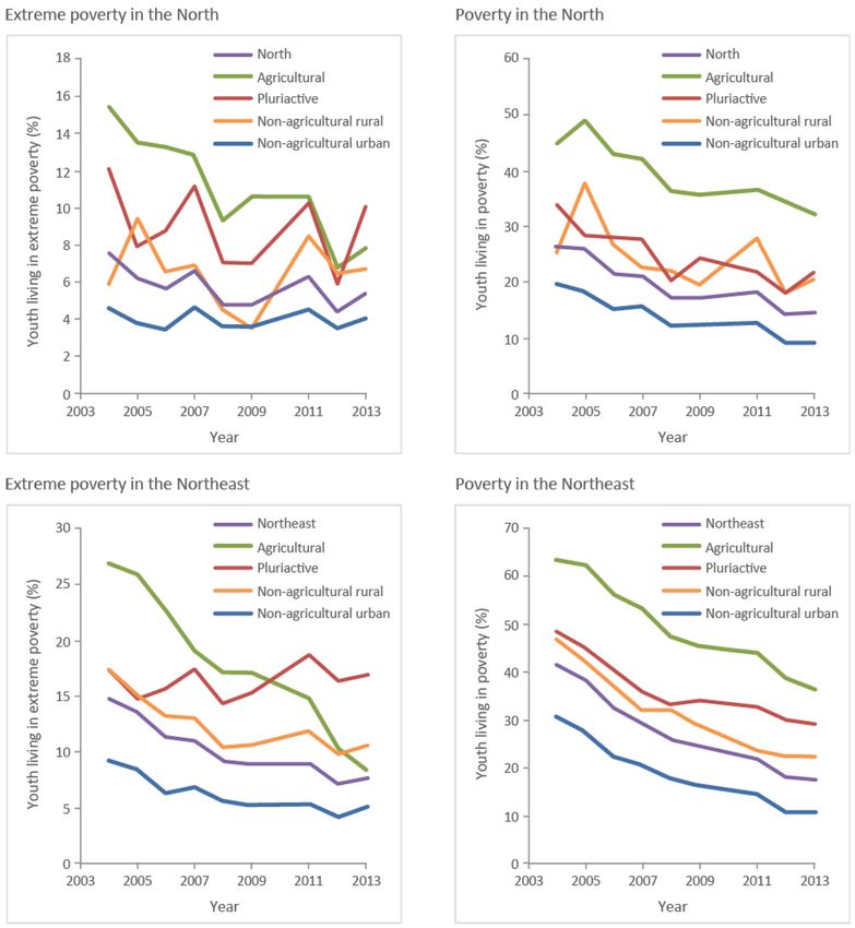
14 International Policy Centre for Inclusive Growth

 In summary, although there is no evidence of an increase in the relative poverty of
households headed by women compared to other families both in the North and in the
Northeast regions, the same cannot be said of extreme poverty. Between 2003 and 2013,
there was an increase in the relative poverty of households headed by women in the North.
However, we must highlight that we did not observe a feminisation of extreme poverty
in the Northeast of Brazil.

 3.2 YOUTH
The insertion of youth into the economic system is a global problem; when we look at rural
poverty, however, young people do not seem to be more vulnerable than any other group.
 Figure 11 shows that the evolution of extreme poverty among young people is very
similar to that of the general population. Extreme poverty has declined sharply among
agricultural households and non-agricultural urban households and remained stable in
pluriactive and non-agricultural rural households. Moreover, the graph for non-extreme
poverty among young people is also very similar to that for the general population.

FIGURE 11
Percentage of youth living in poverty and extreme poverty in Brazil

Source: PNAD, selected years.
IFAD Strategy for Brazil 2016-2021 and Serie of Studies on Rural Poverty 15

 What do poverty and extreme poverty among young people look like in the
North and Northeast?

FIGURE 12
Percentage of youth living in poverty and extreme poverty – North and Northeast

Source: PNAD, selected years.
16 International Policy Centre for Inclusive Growth

 In the North, the figures begin to get noisy due to the small sample size, but overall the
trends are the same as for general poverty. For the Northeast, again, the same analysis applies.
The behaviour of poverty and extreme poverty among young people is the same as among
the Brazilian population as a whole.
 The fact that there are no significant differences in the evolution of poverty and
extreme poverty when comparing youth and the general population does not mean that
there are no important specificities for young people in the North and Northeast; it just
means that they are not directly related to poverty. Young people face significant
unemployment problems that highlight the difficulties faced by the economic system in
quickly integrating them. Young people face important challenges in education, as the
school system has not been able to keep pace with changes in connectivity. As a group,
young people are notoriously at risk of certain criminal behaviours. All these issues are
important challenges for public policies aimed at the youth but are not directly linked to
the status of poverty as defined by the poverty lines used here.

 3.3 HOUSEHOLD (PRIVATE) INFRASTRUCTURE AND ACCESS TO PUBLIC SERVICES
 (PUBLIC INFRASTRUCTURE)
We know that defining poverty purely in terms of income fails to account for all that poor
people lack. As shown in Figure 13, there are still challenges, both in terms of the Brazilian
population’s access to certain goods—such as refrigerators and computers—as well as
access to public infrastructure services such as sewage and piped water.
 We calculated considerably more indicators than will be shown in this section: a total
of four public infrastructure indicators and nine private infrastructure indicators. Many of
them—such as access to electricity or stove ownership—were nearly universal in Brazil
even in 2004. Basically, two public infrastructure indicators and two private infrastructure
indicators showed the biggest changes in terms of the population’s access to them.
However, access to sewage—one of the ‘more dynamic’ indicators—has changed
very slowly.
 Figure 13.1 shows the percentage of households with access to public and private
infrastructure (sewage, piped water, refrigerator, computer) in 2004, 2009 and 2013.
Figures 13.2 and 13.3 show the figures for the North and Northeast regions, respectively.
 The increase in the population’s access to private infrastructure greatly surpasses the
increase in access to public infrastructure. Specifically, universal sewage coverage—either
by pipe or by means of a septic tank—remains a challenge. The population’s access to
piped water has progressed more than its access to sewage.
 The same pattern holds true in the North: over time, there have been more significant
increases in access to private household infrastructure than in access to public infrastructure,
with particularly serious deficiencies in the population’s access to sanitation. Between 2004
and 2013, the proportion of agricultural households with refrigerators increased from
42 per cent to 78 per cent, while their access to sewage rose from 20 per cent to 26 per cent.
The remaining household types demonstrate similar trends, although with greater access to
infrastructure—both private and public—than agricultural households.
IFAD Strategy for Brazil 2016-2021 and Serie of Studies on Rural Poverty 17

FIGURE 13.1
Public and household infrastructure in Brazil, 2004, 2009 and 2013

Source: PNAD, selected years.
18 International Policy Centre for Inclusive Growth

FIGURE 13.2
Public and household infrastructure in the North, 2004, 2009 and 2013

Source: PNAD, selected years.

 Results were better in the Northeast. This region boasts greater access to public
infrastructure than the North, probably because governments in the Northeast do not have
to cover the vast distances that governments in the North have to cover. The Northeast
also boasts other advances in addition to greater access to public infrastructure. The access
of agricultural households to sewage increased from 24 per cent to 36 per cent between
2004 and 2013, placing the Northeast 10 percentage points ahead of the North, which is a
relatively richer region. Among urban households, access is at 72 per cent, against 67 per
cent in the North. Even so, coverage rates as low as 36 per cent for agricultural households
and 72 per cent for urban households are unacceptable for public services.
IFAD Strategy for Brazil 2016-2021 and Serie of Studies on Rural Poverty 19

FIGURE 13.3
Public and household infrastructure in the Northeast, 2004, 2009 and 2013

Source: PNAD, selected years.

 The increase in access to private infrastructure in the Northeast is close to the increase
seen in the North. In terms of refrigerator ownership, 89 per cent of households in the
Northeast own at least one refrigerator; in the North, this percentage is 78 per cent,
and in Brazil as a whole, 92 per cent. This difference is slightly larger than the income
gap between the regions.
 The main conclusion is that access to infrastructure—both public and private—
is extremely relevant to people living in poverty and extreme poverty; therefore, access
to infrastructure must be prioritised.
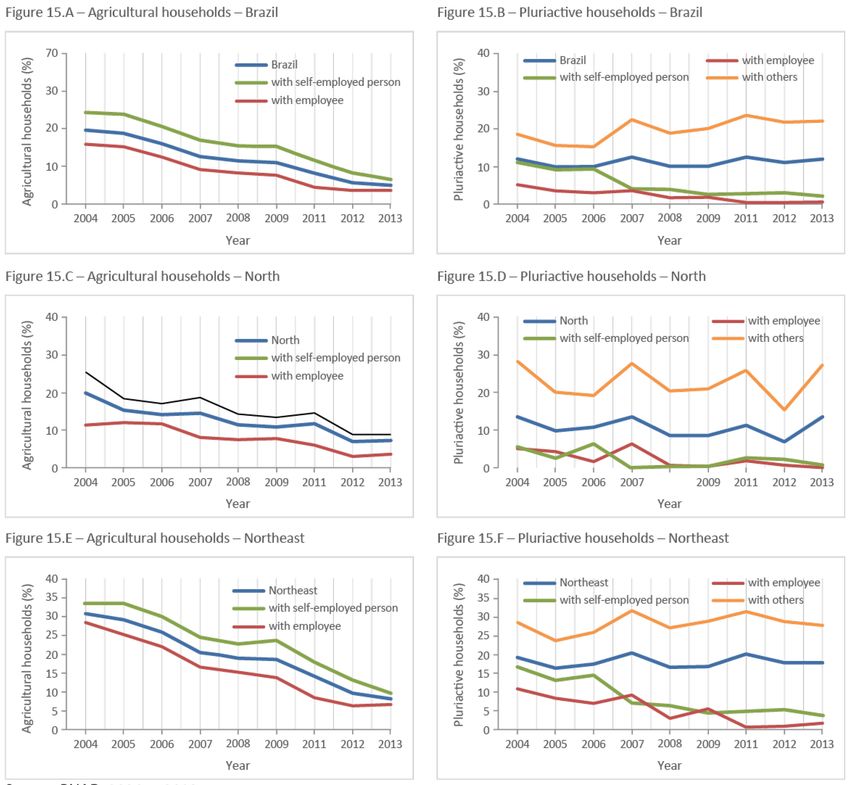
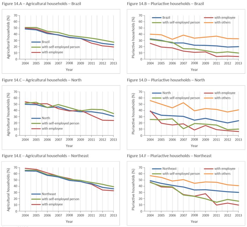
20 International Policy Centre for Inclusive Growth

 3.4 AGRICULTURAL AND PLURIACTIVE HOUSEHOLDS ACCORDING TO THE
 OCCUPATION OF ITS MEMBERS
In this section, agricultural and pluriactive households are broken down into four categories
according to the occupation of their members:
 • households with at least one employer;
 • those with at least one self-employed individual;
 • those with at least one wage-earning employee; and
 • households with other types of occupation.

 According to this breakdown, agricultural households are divided into three categories
(households with an employer; those with a self-employed individual; and those with an
employed wage earner), whereas pluriactive households are divided into four categories
(households with an employer; those with a self-employed individual; those with an employed
wage earner; and households with other types of occupations).
 Note that if there is an employer in a given household, for example, it does not preclude
the possibility of an employee also living in the same household. As such, we can analyse both
the incidence of poverty as well as the main problems that cause it, taking into account, in a
sense, the status of occupations existent in households engaged in agricultural activities.
This analysis is important because one might expect that residents of households with
employers would enjoy better socio-economic conditions than those in households without
employers, for example. As in the rest of this poverty profile, we must note that our units of
analysis are the individuals who reside in these households—and not the households per se.
 Figure 14 shows the evolution of the incidence of poverty between 2004 and 2013 among
residents in agricultural and pluriactive households and their occupational subgroups for Brazil
as a whole and for the North and Northeast regions. We did not analyse households with
employers for two reasons. This group accounts for an extremely low proportion of the
population living in both agricultural and pluriactive households in Brazil (3.23 per cent and
1.83 per cent, respectively), and the incidence of poverty in this group is almost residual.
 Figure 14 shows that the decrease in the incidence of poverty among agricultural
households (Figures 14.A, 14.C and 14.E) was marked by a greater reduction in poverty
for agricultural households with employed wage earners than for households with self-
employed individuals. This happened in both the North and Northeast regions. The same
situation occurs when we compare pluriactive households with self-employed individuals
with those with employees. When analysing the pluriactive households (Figures 14.B, 14.D
and 14.F), however, we must highlight the category of households whose members hold
other types of occupation (i.e. those who are not employers, self-employed individuals or
employees). This is the group that saw the least amount of poverty reduction between
2004 and 2013. To mention one example, while poverty among pluriactive households
with employees in the Northeast fell from 47 per cent in 2004 to 10.1 per cent in 2013,
among households with other types of occupation the decline was much less significant
during the same period (from 57.5 per cent to 41.2 per cent).
IFAD Strategy for Brazil 2016-2021 and Serie of Studies on Rural Poverty 21

FIGURE 14
Percentage of the population living in agricultural and pluriactive households who are poor –
Brazil and the North and Northeast regions, 2004–2013

Source: PNAD, 2004 to 2013.
22 International Policy Centre for Inclusive Growth

 Figure 15 shows the evolution of the incidence of extreme poverty between 2004 and
2013 for residents in agricultural and pluriactive households and their occupational subgroups
for Brazil as a whole and in the North and Northeast regions.

FIGURE 15
Percentage of the population living in agricultural and pluriactive households who are
extremely poor – Brazil and the North and Northeast regions, 2004–2013

Source: PNAD, 2004 to 2013.

 The group of pluriactive households in the ‘other’ category stands out in the analysis
of extreme poverty. This is the only group in which the incidence of extreme poverty not
only fails to decline but even shows an upward trend for Brazil as a whole. In the North and
Northeast regions between 2004 and 2013 the proportion of individuals living in pluriactive
households with other types of occupations (who are not employers, self-employed individuals
or employees) who were poor remained almost constant, at around 27 per cent and
28 per cent, respectively, of the population.
IFAD Strategy for Brazil 2016-2021 and Serie of Studies on Rural Poverty 23

FIGURE 16
Agricultural households (all and those living in extreme poverty) according to their main challenges –
Brazil and North and Northeast regions, 2004 and 2013

Source: PNAD, 2004 to 2013.
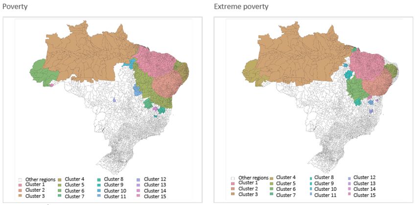
24 International Policy Centre for Inclusive Growth

 To better describe the characteristics of poverty, we must briefly characterise the residents
in agricultural households who are considered extremely poor according to variables that
define their main needs. These variables are: 1) percentage of people living in households
with insufficient land (area is smaller than the average Fiscal Module of the State);
2) percentage of people living in households with no beneficiaries of the Bolsa Família
programme; 3) percentage of people living in households with one or more elderly individual
but where no one receives retirement or other pensions from the Federal Government;
4) percentage of people without signed Employment Cards (informal work); 5) percentage
economically active persons seeking employment during the reference week.
 Figure 16 shows that a lack of access to land is a widespread issue in Brazil: more than
three quarters of the population live in agricultural households with land considered
insufficient (approximately 81 per cent in both 2004 and 2013). Between 2004 and 2013,
there was a decline in the proportion of people living in households without Bolsa Família
beneficiaries (from 41 per cent to 30 per cent). In the Northeast, this decline was even greater:
from 37 per cent to 22 per cent, consistent with the programme’s high rate of coverage in the
region. Only for households living in extreme poverty is there an increase in the proportion of
people living in households with elderly individuals without retirement and/or other pensions;
for the total population living in agricultural households, this figure shows a decrease in both
regions. This, combined with the high rate of coverage of Bolsa Família, may indicate that more
is needed in addition to Bolsa Família benefits to lift households out of extreme poverty.
 Informal labour declined among residents in agricultural households in Brazil (although
labour informality remains high: 60.5 per cent in 2013). Among those living in extreme poverty,
however, the level of informality is increasing (nearly all of them—99 per cent—worked in the
informal market in 2013). With regard to underemployment (people working fewer than 20
hours a week) and the search for employment, once again the extremely poor population in
agricultural households is overrepresented. In 2013, 17 per cent of residents in agricultural
households were underemployed. This proportion rises to 25 per cent in the case of those
living in extreme poverty. The members of extremely poor households are also the people
who most sought employment in 2013: 15.7 per cent of them, compared to 7.2 per cent
of the total population living in agricultural households.

 4 POVERTY AND EXTREME POVERTY AT THE MUNICIPAL LEVEL
 BASED ON THE 2010 CENSUS
When dealing with thousands of municipalities, few tools are as useful and convincing as
poverty maps. Colour-coded maps can convey a far more satisfactory idea of where poor
households are located than tables or graphs.
 Figure 17 clearly shows that poverty is essentially a problem of the North and Northeast
regions. Few municipalities in the other three regions of Brazil show poverty rates higher
than 30 per cent (5.5 per cent of the municipalities located in the South, Southeast and
Centre-West regions), and many have rates lower than 15 per cent (about 26 per cent of these
municipalities). On the other hand, in the North and Northeast regions most municipalities
show rates above 30 per cent (67 per cent and 86 per cent of municipalities, respectively).
IFAD Strategy for Brazil 2016-2021 and Serie of Studies on Rural Poverty 25

FIGURE 17
Percentage of people living in poverty and extreme poverty by municipality – Brazil, 2010

Source: Population census 2010.

FIGURE 18
Percentage of people living in poverty by municipality, by demographic group – Brazil, 2010

Source: Population census 2010.
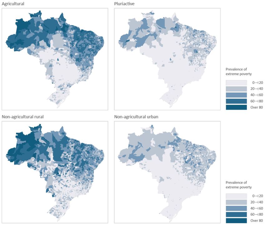
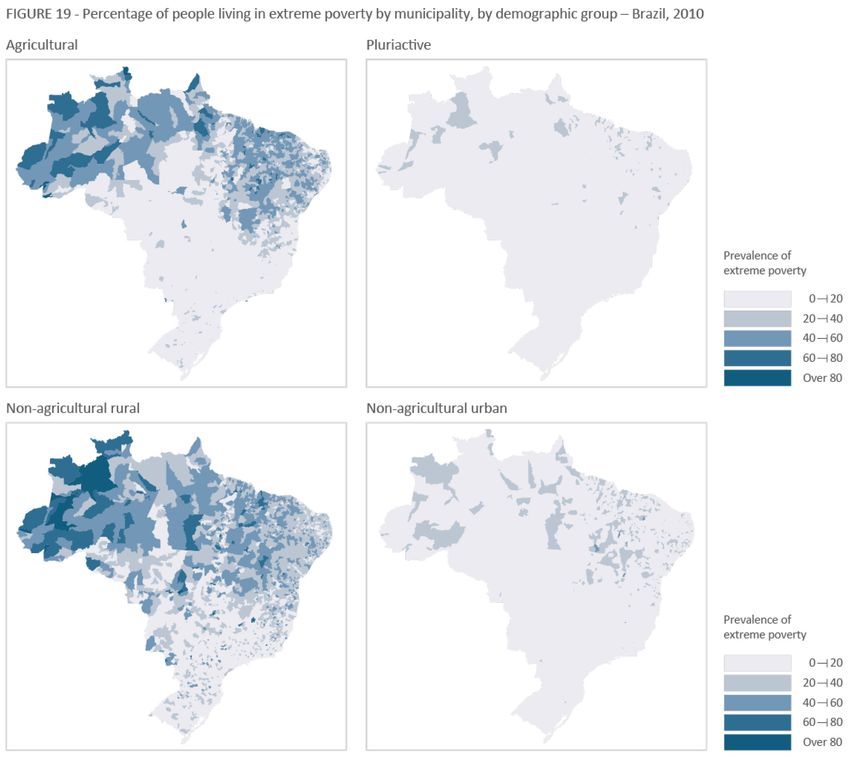
26 International Policy Centre for Inclusive Growth

 In the North and Northeast, however, the situation is quite different. Many municipalities
show poverty rates higher than 60 per cent; in some municipalities they may be as high as
90 per cent. This can be seen in the areas of the map coloured in darker blue in the North and
Northeast. Especially notable are the very poor areas in the northwest of the North and the
northwest of the Northeast. These are the poorest of the poor areas.
 The story of extreme poverty is essentially the same as the story of poverty. The North
and Northeast see much more extreme poverty, and the northwest parts of these two regions
contain the highest numbers of extremely poor households.
 When we analyse the rural dimension, we observe that the differences are even more
pronounced in certain cases. The maps show that the differences are very pronounced among
agricultural households. The dark blue area in the western Amazon is especially alarming. The state
of Maranhão, in the northwest of the Northeast, also shows very high levels of agricultural poverty.
 The differences within non-agricultural households are less significant, although they do
exist. Of special note is the fact that the differences are much smaller among non-agricultural
rural households. Poverty levels of agricultural households in the South and Centre-West are
closer to those in the North and Northeast than for other types of households.
 Finally, what do the extreme poverty maps look like?

FIGURE 19
Percentage of people living in extreme poverty by municipality, by demographic group – Brazil, 2010

Source: Population census 2010.
IFAD Strategy for Brazil 2016-2021 and Serie of Studies on Rural Poverty 27

 The extreme poverty maps have lighter shades. This is not surprising, since the extreme
poverty line is lower, which means that the proportion of extremely poor individuals will
always be lower. Disregarding this fact, the main results remain: there are marked differences
among agricultural households and greater regional homogeneity in pluriactive and
non-agricultural urban households.
 These maps clearly show that the problem of rural poverty in Brazil is largely a problem
of agricultural households in the North and Northeast. In this sense, it is also important to
look into the differences in family farming between the North and Northeast regions and in
comparison with the rest of Brazil. We used the information available from the 2006 Census
of Agricultureto do so.
 So far, this study leads us to the following conclusions: 1) much of the decline in rural
poverty is due to the decline in poverty among agricultural households; 2) there are marked
differences—both in poverty and in extreme poverty—between the North and Northeast
and the other regions of the country; and 3) nowhere are the differences as striking as in
agricultural households.
 These three findings demonstrate that investing in family farming is of paramount
importance to reducing extreme poverty. Figures 1 and 2 show that it can be done, and
Figures 18 and 19 show how relevant this is to reducing the differences in poverty rates
between regions.
 Figure 20 shows what the information available from the 2006 Census of Agriculture tells us
about the differences in family farming between the North and Northeast and the rest of Brazil.

FIGURE 20
Capitalisation indicators for family farming establishments – Brazil, 2006

Source: 2006 Agricultural Census.

 Family farming is undercapitalised in the North and Northeast regions. Figure 20 shows
two indicators of capital in agriculture: the percentage of family farming establishments with
funding (20.A) and the average number of tractors per family farming establishment (20.B).
28 International Policy Centre for Inclusive Growth

These two maps are like mirror images of Figures 18.A and 19.A, which show the rates of
poverty and extreme poverty among agricultural households.
 In other words, both maps show the importance of capitalising family farming. Although
correlation certainly does not imply causation, Figures 20.A and 20.B highlight the enormous
importance of capitalising family farming.

 4.1 SPATIAL CONGLOMERATES OF POVERTY AND EXTREME POVERTY IN
 AGRICULTURAL AND RURAL HOUSEHOLDS IN THE NORTH AND NORTHEAST
As we have seen, poverty and extreme poverty in Brazil are markedly more intense in the
North and Northeast regions. Based on data from the 2010 census, just over 11 million
(about 65 per cent) of the nearly 17 million Brazilians living in extreme poverty (monthly
household income per capita below BRL70) live in the North or the Northeast, causing the
extreme poverty rate (proportion of people living below the extreme poverty line) in this
region to reach 16 per cent, compared to 3 per cent in the South, 5 per cent in the Southeast
and about 9 per cent nationwide.
 Also of note is the fact that just over 6.5 million (60 per cent) of the 11 million people
living below the extreme poverty line in these regions live in households classified as
agricultural or non-agricultural households located in rural areas. The rate of extreme poverty
in these types of household is 28 per cent, compared to 16 per cent for all households in the
region. Similar trends may be observed in the distribution of poor people (monthly household
income per capita below BRL140) among these strata of production and/or household status.
This highlights the importance of this group of households to the poverty observed in the
North and Northeast regions.
 Given these observations, the work documented here focuses mainly on families
who carry out agricultural activities (the households previously defined as agricultural
households and pluriactive households are taken together in the analysis of this section)
and non-agricultural households in rural areas. More specifically, the main objective is to
describe the spatial distribution of the incidence of poverty and extreme poverty in these
strata and to investigate the existence of poverty conglomerates—contiguous sets of
municipalities where the rate is higher than in other regions.
 The importance of this effort lies in the rationale that the existence of spatial
conglomerates (clusters) of a given phenomenon is most likely associated with local causes of
various types. This effort was also important for identifying priority regions for implementing
public policies that are easy to disseminate to neighbouring municipalities while taking into
account the social, political, economic and geographical characteristics of each region.
 Research on spatial conglomerates of poverty is nothing new. Collado (2004) uses
Kulldorff’s scan statistic (1997) to detect poverty conglomerates in Costa Rica. Amarasinghe et
al. (2005) conducted a study to detect poverty clusters in Sri Lanka. Medeiros and Neto (2010)
use 2010 census data to analyse the spatial determinants of extreme poverty in the state of
Ceará and also perform an exercise to detect spatial clusters. Similar works have detected
clusters in the Northeast (Silva et al. 2013) and in the state of Minas Gerais (Romero 2006).
 Almost all of the papers cited detect spatial poverty clusters using Local Indicators
of Spatial Association (LISA) to identify conglomerates. Additionally, most papers focus
on poverty in all households. The difference of this study lies mainly in its focus on
IFAD Strategy for Brazil 2016-2021 and Serie of Studies on Rural Poverty 29 non-agricultural rural families and agricultural families. Another difference worth mentioning is its use of an alternative procedure to that used by most researchers, which is advantageous mainly because it is a semi-parametric methodology (with rather flexible assumptions, not ‘tied’ to normality assumptions of little credibility). In the following section we shall briefly describe the LISA indicator and the scan statistic for detecting spatial clusters. We will then present the general results and some of the characteristics of the extreme poverty clusters detected among people living in agricultural households—more specifically, compositional and structural data on family farming and PRONAF activities. Two methodologies were used to identify poverty and extreme poverty conglomerates among agricultural and rural households in the North and Northeast: the scan statistic with circular windows and Moran’s spatial autocorrelation indicator, from which the local LISA indicator is derived. The first technique, developed by Kulldorff (1997), came about in the context of epidemic outbreak detection, although it has since been used in various contexts outside epidemiology. It is an intensive and non-parametric computational procedure. Moran’s indicator follows the same logic as first-order temporal autocorrelation, but applied to the spatial context. a) An statistic As originally proposed, the scan procedure ‘sweeps’ the map iteratively in search of areas where a given phenomenon occurs with greater probability than in other regions. Each iteration begins in a municipality within the map, from which a window extends and proceeds to encompass other cities. For every new municipality encompassed by this window, a likelihood ratio is calculated. When the window around the municipality contains the maximum number of predefined regions, the process restarts by centring the window on another municipality. The procedure ends when all municipalities have been used as centres for windows. The likelihood ratio (LR) calculated in each LR zone is given by c C −c z c z C − cz LR = z I(cz μz ) μ z C − μ Z where: • c z is the number of poor people within the window; • μz is the number of poor people that one would expect to find within the region if there were no conglomerate on the map. In this case, μz = pN , where p is the poverty rate across the entire map, and N it is the total population; • C is the total number of poor people in the region; and • a cluster is defined as the window with the largest LR. However, the possibility exists that this concentration is just a probable fluctuation. To test the statistical significance of this cluster, we have carried out a Monte Carlo experiment generating random values for each municipality based on a Poisson distribution with an average μz .
30 International Policy Centre for Inclusive Growth

 Though this method may be powerful, its accuracy depends largely on the format of the
windows defining each zone. The simplest format, used in this study as a preliminary exercise
for future enhancements, is a circular window. 6
 b) Moran’s global indicator I and LISA indicators
 Moran’s indicator I is a measure of spatial autocorrelation. It calculates the degree of linear
dependence between the value observed in a municipality and the values of its neighbours.
The index ranges from -1 to 1. Positive values indicate that regions with the highest poverty
rates tend to have neighbours whose poverty rates are also high (and neighbours with low
rates tend to have neighbours with values in the same trend). Negative values indicate a
pattern in which municipalities with high rates tend to have neighbours with low rates
(and vice versa). Moran’s global indicator I is given by:

 n n

 n
 ∑∑ w ( y − y )(y
 i=1 j =1
 ij i j − y)
 I= n n n

 ∑∑ wij ∑ (y − y)
 2
 i
 i=1 j =1 i=1

where:
n is the total number of municipalities in the region;
yi is the poverty (or extreme poverty) index for municipality i;
y is the regional average; and
wij is defined so that its value is 1 if municipalities i and j are neighbours, and 0 otherwise.
 In other words, Moran’s global index is a Pearson correlation between the values of
municipalities and those of their neighbours. The null hypothesis states that values occur
randomly in the map (I = 0), with no specific spatial pattern. The significance of the global
index can be tested via a parametric method, assuming the normality of the variable in
question, or via a Monte Carlo simulation, based on several random orders of the indicator.
 The indicator I, however, only shows global correlations and does not indicate regions
with positive and/or negative associations. The LISA indicator is used for that purpose:
 n
 ( yi − y )∑ (y j − y )
 j =1
 LISAi = n

 ∑ (y − y)
 2
 j
 j =1

6. This method is quite limited, in a way, as there is a high chance that a conglomerate, if it exists, will not necessarily be
circular. Nevertheless, there are methods with elliptical windows—Kulldorff et al. (2006)—or even irregular windows—
Tango and Takahashi (2005)—available.
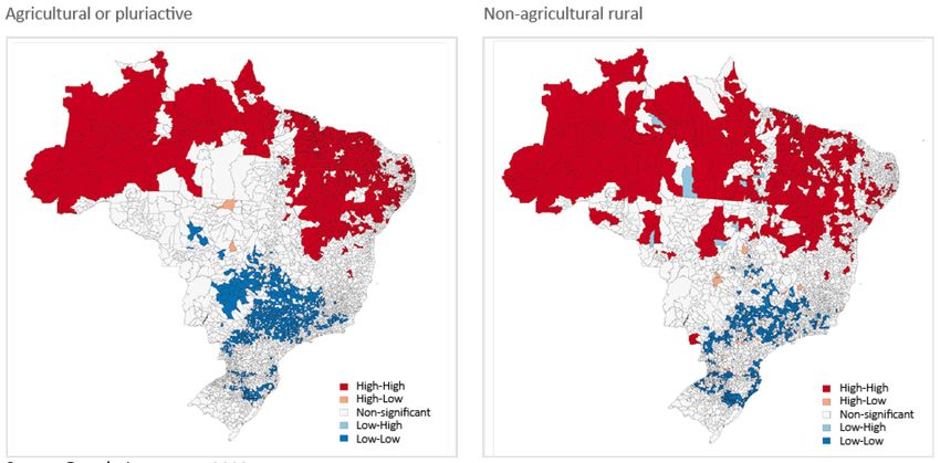
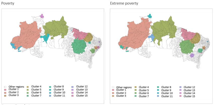
IFAD Strategy for Brazil 2016-2021 and Serie of Studies on Rural Poverty 31

 The LISA indicator for each municipality is the correlation of its value with those of its
neighbours. The local indicator is also statistically tested—parametrically or by simulation—
in a fashion analogous to the global indicator I.
 c) Moran’s mirroring diagram
 The mirroring diagram can be used to verify and classify the spatial association pattern.
We begin by setting standardised values z i . Positive values for z i indicate a poverty rate above
the regional average; negative values indicate a rate below the average. Subsequently, we
define the lag of z i as the neighbours’ average. The mirroring diagram is an z i X lag( z i )
scatter plot. Depending on the municipality’s position in each quadrant, it will be classified in
one of the following groups:
 • High-High Group: the municipality has a poverty rate above the regional
 average, and its neighbours follow this trend, also showing above-average values.
 This corresponds to the first quadrant of the diagram;
 • High-Low Group: the municipal rate is above average, but those of its neighbours
 are below average;
 • Low-High Group: the poverty rate is below average, and neighbours’ poverty rates
 are above average; or
 • Low-Low Group: corresponds to the third quadrant of the diagram, for cases
 in which the municipality has a below-average rate and its neighbours follow
 this trend.

 The main advantage of this method with respect to a circular scan is the fact that here
the conglomerate shape is not limited to a circle. Moreover, we can check for the presence of
‘negative’ clusters, in which the phenomenon under investigation occurs in an opposite
direction. It may be limited, on the other hand, due to its parametric nature and to the fact
that it was applied (at least here) considering only the first-order neighbourhood. Its power
of detection loses strength, as it relies on multiple individual tests with the LISA indicator.
 The scan statistic, in turn, has an interesting property: the most likely cluster is still a
significant conglomerate regardless of the composition of the rest of the map, while local
indicators are strongly influenced by the composition of the rest of the region.

 ANALYSIS OF RESULTS
Moran’s Global Indices: All maps show significant spatial correlation. In both strata (agricultural
and rural households), both the poverty and the extreme poverty rates have a much stronger
spatial relationship than when we consider only the North and Northeast regions, thus
showcasing the disparity of these regions vis-à-vis the rest of the country. Figures 21 and 22
show the mirroring diagrams (standardised value X average of neighbours) of the indicators
observed in the North and Northeast, showing a linear trend between the incidence of poverty
and the average of neighbours.
You can also read