Using fuzzy clustering to reveal recurring spatial patterns in corpora of dialect maps
←
→
Page content transcription
If your browser does not render page correctly, please read the page content below
1

         Using fuzzy clustering to reveal recurring spatial
         patterns in corpora of dialect maps*

         Daniel Meschenmoser & Simon Pröll
         University of Ulm / University of Augsburg

         In this article, a new method to identify groups of spatially similar dialect maps is presented.
         This is done by comparing statistical properties of the maps: the empirical covariance is
         measured for every map in a corpus of dialect maps. Then, the Fuzzy C-Means clustering
         method is applied to these covariance data. Thereby, one is able to detect and measure gradual
         similarities between maps. By employing the method on lexical data from the dialect atlas
         Sprachatlas von Bayerisch-Schwaben, it can be shown that clusters of spatially similar maps
         also share semantic similarities. This method can thus be used for grouping maps based on
         spatial similarities while at the same time indicating patterns of semantic relationships between
         spatially related variables.

         Keywords: dialect corpus, dialectometry, cluster analysis, covariance, semantic categorisation

1. Introduction and objective

While for quite some time “corpus linguistics has largely ignored any spatial dimension
within the texts that it studies” (Gregory & Hardie 2011: 298; see also Adolphs et al.
2011: 307 for a similar comment), recent approaches begin to shift attention accordingly.
These days, spatiality of data – a central topic of sociolinguistics and dialectology – is
increasingly becoming a theme in corpus linguistics as well. New approaches, like those
of Adolphs et al. (2011) or Gregory & Hardie (2011), link corpora to GIS (Geographic
Information System) data or use large text corpora for studies of regional variation, like
Szmrecsanyi (2008, 2011) or Grieve (2009, 2011).
   For the resulting new types of demands on corpora, Adolphs et al. (2011: 318)
postulate that it is vital to be able to effectively search both data and metadata. In this
paper, we propose a method to search the spatial “metadata” in dialect atlases – which
we use as a corpus-like database – for recurring patterns. More specifically, we show
how to automatically find groups of dialect maps that have a similar geographic
structure. This can help to answer ubiquitous variationist questions on which linguistic
features take part in diffusion processes (see e.g. Britain 2002) or which semantic
groups contribute to the structure of a certain dialect. At the same time, we show to
what extent it is possible to regard the data contained in dialect atlases as a corpus.
   Our approach differs from traditional computational dialectology that was developed
at the end of the 19th century, in the wake of the introduction of quantitative methods,
by Carl Haag (cf. Haag 1898). The basic principle of those methods, commonly
subsumed under the term ‘dialectometry’, is that a large quantity of datasets (the usually
hundreds of maps from dialect atlases) is aggregated. The strength therein is that
seemingly “unsystematic” aberrations of single maps are minimised, while only one
kind of information becomes dominant, the one that is common to a large number of
maps (see Nerbonne 2009). This procedure leads to good results if one intends to
distinguish between whole dialects (cf. Nerbonne & Kretzschmar 2003, Goebl 2006).
2

However, the detailed information contained in the individual maps is lost in the
process, i.e. we may know how dialects are distributed, but we do not know why.
Therefore, the objective is to group maps in a way that preserves their individual spatial
and linguistic information, or, in other words to build clusters of identifiable maps that
share similar spatial patterns of variants.
    Here, we present a solution to this problem using a clustering method that compares
the spatial structures of maps via statistical tools. Examples from Southern Germany are
used to exemplify the new approach, but the technique is not restricted to these data; it
is applicable to any kind of spatially distributed information. It allows for treating maps
of (dialect and other) atlases as searchable items of a corpus and for automatically and
objectively grouping them based on their spatial similarities. Because we pre-prepare
the atlas data to resemble usual corpora, this method of identifying patterns in the
metadata can in principle be applied to corpora containing GIS data as well.
    A related technique has recently been introduced in Rumpf et al. (2010), originating
from the same research project. There are crucial differences to our method, though,
which will be further illuminated in Section 3.3. Both the method presented here as well
as the approach by Rumpf et al. (2010) may open up perspectives beyond traditional,
locally bound methods in dialectometry by giving the opportunity to examine structural
similarities of maps independent of concrete, fixed locations. 1

2. Data

2.1 Fusing dialect data, dialect atlases and corpus linguistics

The obvious strong point of linguistic atlases as database is that the geographic
information is very detailed and directly connected to the linguistic data. However, there
are three major differences between the data in dialect atlases and natural language data
common to corpus linguistics that need to be addressed here:
    (a) The total number of items in dialect atlases is relatively low.
    (b) The data of dialect atlases are not “natural” but elicited under controlled
        circumstances.
    (c) The data of dialect atlases are not frequency-based but of categorical nature.
Concerning (a): We share the view of Flowerdew (2004) and Koester (2010) that size is
not the decisive parameter of corpus quality: small corpora have the advantage “that,
unlike with a large corpus, the language is not de-contextualised. On the contrary, there
is a very close link between language and context” (Koester 2010: 74). For dialect
corpora, where the (geographic) context of the data is at the centre of interest, small size
is additionally compensated for by high representativeness of the data due to the next
point, their controlled elicitation.
   Concerning (b): Most dialect atlases are based on data gathered through direct
questioning of older, rural men that were instructed to use the oldest linguistic forms
available to them; thus, the difference between the data in dialect atlases and natural
language corpora is that dialect atlases usually feature controls for many variables:
factors such as age, situation, and even the recorded linguistic items themselves (that are
elicited using a questionnaire) are restricted through the design of the survey itself. As
above, this has a positive impact on the inclusion of context and leads to rather small,
condensed datasets (compared to natural corpora). The finished atlas provides a
diachronic view on variation, as it puts emphasis on forms that have become extinct in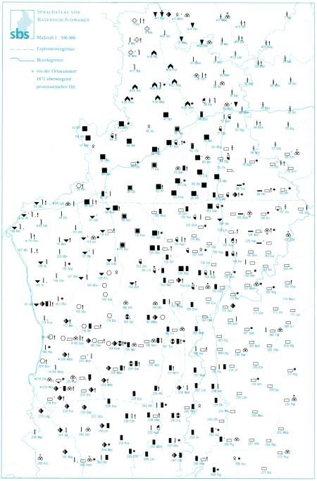
3

contemporary language use. It can thus be regarded as a small, specialised (in the sense
of Flowerdew 2004) corpus on old dialectal forms which are hardly explorable through
the gathering of natural language: historical corpora, e.g. compiled from lower class
letters (see Elspaß 2007), are inevitably concentrated on written language (and thus can
only provide indirect information on a lot of linguistic questions), whereas modern
multimodal/audio corpora cannot (yet) compete with the close-meshed nature of
systematic surveys and are – as absurd as it may seem – too “carefully balanced”
(Flowerdew 2004: 14), that is to say compiled under the premise of representativeness
of the language as a whole, to capture rural dialect forms on the verge of dying out.
    Concerning (c): as Szmrecsanyi (2008, 2011) points out, while corpus work focuses
on the examination of frequencies of phenomena, dialect atlases usually feature
categorical, digital data (see, however, König 1989): on location A, variant x is used,
whereas on location B, variant y is used. Here, we make use of densities of variants (see
below, Section 2.4) and are thus able to work “frequency-based” (Szmrecsanyi 2008:
280), i.e. with continuous values, as well. This enables us to use statistical methods
(common to corpus linguistics) that are not applicable to categorical data on dialect
atlases; thus, atlas data are transformed into a viable object of research for corpus
linguists.

2.2 The Sprachatlas von Bayerisch-Schwaben

For the present paper we exemplify our methods with data from the Sprachatlas von
Bayerisch-Schwaben (SBS), covering the administrative region of Swabia in South
Germany plus smaller parts of Upper Bavaria and Middle Franconia. 2 The data has been
gathered in field interviews on 272 record locations during the 1980s, transcribed on
site using the phonetic transcription system Teuthonista (following Teuchert 1924).
Multiple records at each site for one questionnaire item were possible (instead of letting
the interviewer or the cartographer choose – via introspection – which variant they
consider to be “dominant”). This may make the handling and visualisation of the data
rather complex on the whole, but it consequently allows for a shift of interpretation
from the interviewer and cartographer to the user of the atlas. The original publication
features 13 volumes (plus index) and contains more than 2,700 maps that visualise the
spatial distributions of lexical, phonetic and morphological phenomena. Without the use
of statistical methods, though, it would be impossible to handle and/or investigate so
much data in an objective way and without excessive expenditure of time and resources.
For the original atlas publication, all manual field transcriptions were computer-coded
and stored in the form of one tabular text file for each variable. For our purpose, we
compiled the information from these files (variable, variant, location) into a SQL
database. Thus, as the whole set of data is completely available in digitised form, it is
relatively easy to apply methods from spatial statistics to it (at least compared to many
other dialect atlases for which the data has not been digitised).
    For this paper, we have restricted ourselves on the 6 volumes that contain lexical
information (on a total number of 736 maps), therefore the interpretations drawn from
the methods presented here are of semantic nature. Concentration on the other volumes
would allow other types of questions, naturally; with regard to phonetic data, for
example, it would become possible to examine patterns like chain shifts (cf. Wiesinger
1982, Gordon 2002).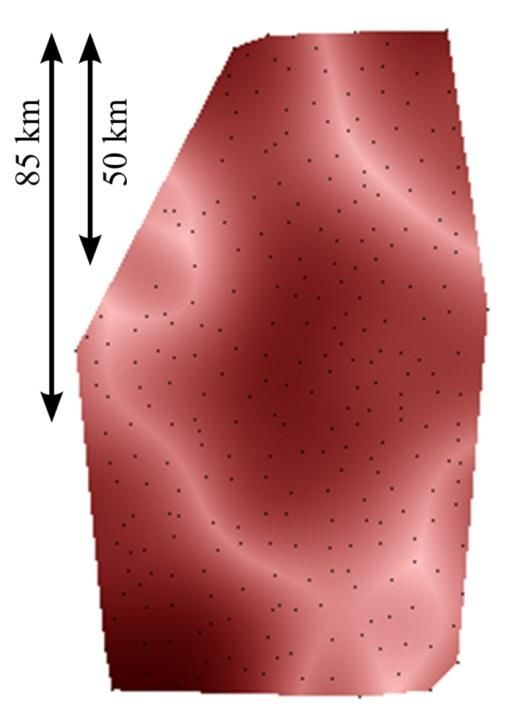
4

2.3 Topics of the lexical volumes

The 6 volumes we are dealing with are each divided into smaller categories. An
overview is given in Table 1. In addition to 29 semantic categories, there is an extra
category “adverbs” plus a small assemblage of single maps, grouped under the term
“miscellaneous maps”.
Table 1. Categories of the lexical volumes (as specified in the volumes themselves; translated from
German, numbered progressively)
            V                o                l                u                 m                 e
            2                8               10                11                12               13
           (1)              (5)              (12)              (18)            (22)              (27)
 C     the human      the farmhouse       children’s     cattle and dairy     terrain         wood and
          body              (6)             games          processing          (23)            timber
  o       (2)         habitation and        (13)              (19)           soil and            (28)
      physical and      furnishing        household        pig, goat,       cultivation         fences
       emotional           (7)              (14)          sheep, horse          (24)             (29)
  n   expressions       weather           nutrition,           (20)         fertilisation     transport
          (3)          phenomena         cooking and     poultry keeping       (25)               (30)
       community            (8)            baking        and beekeeping     hay harvest      baskets, jars
  t
           (4)         wild animals          (15)             (21)             (26)           and bearer
        clothing            (9)          peasants and         pets             crop             frames
  e                  plants, fruit and   agricultural
                        vegetables        labourers

                           (10)             (16)
  n                       must        division of time
                      production (for   and greeting
                        beverages)          (17)                                              (31)
  t                                       adverbs
                           (11)                                                       miscellaneous maps
                         flowers

As can be seen, while the grouping of the topics is far from random, the individual
volumes are still rather heterogeneous.3 The single categories share this problem; a fair
share of their maps might be attributed to other categories as well. We will address this
problem when dealing with our results in Section 4.

2.4 Preparation for our purpose

The original point-symbol maps (see Figure 1a for an example) that are contained in the
volumes of the SBS cannot be used directly for statistical tests. Therefore, Rumpf et al.
(2009) devised techniques for transforming point-symbol maps into so-called area-class
maps using density estimation. Figure 1b shows an example of such an area-class map
corresponding to the point-symbol map in Figure 1a. The major difference between both
types of maps is that while point-symbol maps display concrete records at the location
they were taken, the area-class maps visualise the probabilities of variants in space, i.e.
the likeliness that informants at a given point of the area use a specific form. Using
those density values instead of the original categorical data brings us closer to common
corpus structures and circumvents the respective issues that we addressed above (see
Section 2.1). Different prevalent variants are indicated by different colour hues. The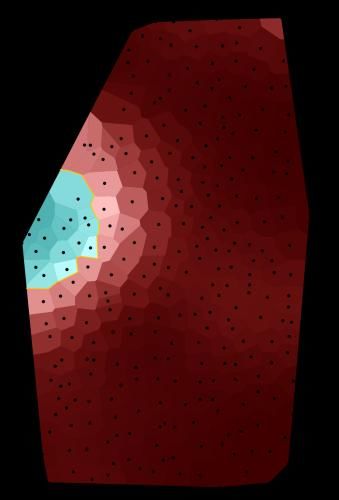
5

lightness denotes the degree of dominance of a variant: areas where variants are
intermixed are displayed lighter whereas areas with high ‘homogeneity’, i.e. where one
variant dominates clearly over the others, are darker. Ideally, the darkest spots indicate
that there is just one variant present (cf. Rumpf et al. 2009 for further details on the
generation of area-class maps and their interpretation). We take one step further and
neglect the colour hue, which leaves us with a map where only the prevalence of the
variants is shown; we call these monochromatic maps ‘prevalence maps’. At each point
of the map, the lightness indicates the likeliness that informants at this point use the
prevalent form. The darker the map at a given point, the more likely an informant uses
the prevalent form. Figure 1c shows the prevalence map corresponding to the area-class
map in Figure 1b. The small black dots in the area-class map as well as in the
prevalence map denote the record locations. The area-class maps consist of small cells
whereas the prevalence map is smoother. This was achieved by computing the
probabilities not only at the record locations but on all points of a dense rectangular grid.
The prevalence maps no longer allow distinguishing the different variants, which is not
necessary for our purpose. As can be seen in Figure 1, it is sufficient to differentiate
between dark and light areas, because borders between the different dominant variants
of Figure 1b are still visually salient as light bands in the prevalence map (Figure 1c).
The reason for this is obvious: borders between variants are much “fuzzier” than
isogloss techniques imply (cf. Naumann 1982: 686, Händler & Wiegand 1982). Often,
there is a transitional area from one variant to the other, where speakers use both
variants. In those transition areas no variant is highly dominant, which leads to lighter
belts in the maps.

    (a) Original point-symbol              (b) Area-class map                 (c) Prevalence map
    map 2005 Beule (“bump”)            corresponding to the point-         corresponding to the area-
  from the SBS (Vol. 2, p. 311)         symbol map 2005 Beule                class map 2005 Beule
Figure 1. Two stage transformation of the original map (left) into the prevalence map (right)

These prevalence maps form the basis for employing statistical methods on dialect data.
In principle, every possible form of spatially distributed data (be it of linguistic, cultural,
geographic or economic origin) can be transformed this way.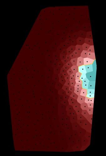
6

3. Methodology

3.1 Cluster analysis as a method for accessing dialect corpora

As explained in the preliminary chapter, “traditional” quantitative approaches to
dialectology (cf. the concise overview in Heeringa 2004: 14ff.) investigate differences
between dialects as a whole by aggregating linguistic features and measuring the
linguistic distance between two places. In contrast to this approach, we consider the
collection of maps as a searchable corpus; our method is aimed at preserving the
information contained in single maps and at keeping it accessible through every step
rather than aggregating it. From this point of view, our approach is dependent on the
quality of our corpus search methods, i.e. how precisely we can retrieve one single piece
of information and compare it to other pieces.
   Anderwald & Szmrecsanyi (2009: 1136) see a need for improvement on search
methods in dialect corpora, as “[i]t is fair to say […] that current corpus technology – as
employed in corpus-based dialectology – is not especially well geared to deal with
dialect data”. However, their (justified) criticism is based on techniques that use plain
text and records of spoken language as corpus items. In these “identity”-based systems,
an investigator would need complete a priori knowledge over the discrete typographic
or transcriptorial idiosyncrasies of every single item he or she is searching for (cf.
Andersen 2010: 557). Obviously, for the fine phonetic transcriptions of dialectology this
is an impossible postulate. We circumvent these problems by not searching for
(identical) structure in text, but (similar) structure in space. By applying fuzzy statistical
methods on whole dialect maps, we are not bound to identical items in a search process
but we have the freedom to search for similar structures; a statistically-based system
allows for continua of resemblance. Thus, employing methods of cluster analysis on
statistical properties of the single maps is a rather “natural” choice.
   The general principle and purpose of cluster analysis is to categorise one big dataset
into smaller subsets, where each subset is (a) as homogeneous as possible in itself with
respect to certain criteria and (b) as distinct as possible in comparison to the other
subsets. In our case, we intend to create groups of maps that exhibit highly similar
structural properties while looking most distinct from all other groups. The similarity of
two maps is measured by the covariance function as will be explained in detail in the
next chapter.

3.2 Covariance

The covariance describes the relation of two random variables and and is denoted
by             . It shows high positive values if the quantities tend to behave similarly in
the sense that high values of imply high values of and low values of imply low
values of . The covariance takes low (i.e. negative) values if the quantities behave
contrarily, i.e. if high values of frequently occur with low values of and vice versa
(see e.g. Sachs 2003). If the quantities of interest are located on a map, the covariance
additionally depends on the positions of the two quantities.
   In the following, we assume that the statistical properties of the data are – in
mathematical terms – invariant with respect to translations and rotations; i.e. we ignore
the concrete positions of the linguistic data (the places of the individual records) in
favour of a relative, abstract distributional pattern of variants. This implies in particular
7

that the covariance does not depend on the position of the quantities of interest but only
on their distance. In other words, we consider only the average covariance of all
quantities with a given distance in a map and denote it by           . It can be regarded
                                           4,5
as a function depending on the distance. According to Wackernagel (1998), the
empirical covariance for a given distance can be computed by

Here, the prevalence at location is denoted by       and the mean prevalence is given
by . Furthermore,            denotes the distance class of point pairs with distance
approximately . It is defined by

                                                                                ,

where is the rectangular grid of locations where the prevalence was measured. The
parameter controls the accuracy and the smoothness of the method. We put                  ,
which corresponds to rounding the distance between two locations to kilometres.
   The covariance can be measured for all distances from 0 to 162.6 km, which is the
maximal distance occurring in the data (covering the span from the location Kreuzthal
in the southwest to the location Raitenbuch in the northeastern corner of the area).
However, to get reliable results, a sufficient number of point pairs with a given distance
is necessary. For large distances in the map, the number of possible point pairs goes
down. Thus, we compute the covariance only for distances from 0 to 120 km. As there
are only relatively few pairs with a distance greater than 120 km, the covariance would
not be overly meaningful for those distances.

 (a) Prevalence map corresponding to       (b) Empirical covariance function for map 8103 Gießkanne
 map 8103 Gießkanne (“watering can”)
Figure 2. Example for a prevalence map and its corresponding empirical covariance function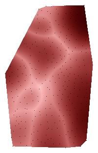
8

Figure 2b shows the empirical covariance function computed for map 8103 Gießkanne
(“watering can”) shown in Figure 2a. Obviously, the covariance is maximal for very
small distances as it is very likely that at a short distance the dominance of a variant
does not change very much. The empirical covariance function attains its minimum at a
distance where there are many dark/light point pairs in the prevalence map (remember
that the black dots are the record locations and are printed for reference only). Here, this
is a distance of about 50 km, which is indicated by an arrow in the prevalence map for
comparison. Of course, there are also dark/dark or light/light point pairs at a distance of
50 km, but they are a minority compared to dark/light point pairs. Further, there is a
second (local) maximum at a distance where many dark/dark or light/light point pairs
occur. For this map, this is a distance of about 85 km as this is approximately the
diameter of the dark region in the middle of the prevalence map.
    The empirical covariance functions may differ considerably; see Figure 3 for three
random examples of prevalence maps together with their corresponding empirical
covariance.

 (a) Prevalence map corresponding to the point-   (b) Empirical covariance function for map 2119
  symbol map 2119 Trauzeuge des Bräutigams                  Trauzeuge des Bräutigams
                (“groomsman”)

 (c) Prevalence map corresponding to the point-   (d) Empirical covariance function for map 12055
     symbol map 12055 zweiter Grasschnitt                        zweiter Grasschnitt
                 (“aftergrass”)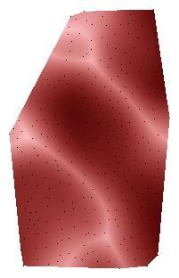
9
(e) Prevalence map corresponding to the point- (f) Empirical covariance function for map 13048
symbol map 13048 mechanische Sägemühle mechanische Sägemühle
(“mechanic timber mill”)
Figure 3. Comparison between various prevalence maps and their corresponding empirical covariance
functions
It can be seen that the main differences between the three empirical covariance
functions are:
The value at distance zero, i.e. the sample variance.
The number of local minima and maxima and the distances where they occur.
In Figure 3b and Figure 3d, the variance is relatively high (compared to Figure 3f),
because the corresponding prevalence maps Figure 3a and Figure 3c feature very light
as well as very dark areas, i.e. the prevalence shows high variability. In Figure 3b and
Figure 3d, the (first) minimum of the empirical covariance function is at a distance of
about 40 km, which is approximately the distance between the very light and the very
dark areas in the corresponding prevalence maps. In contrast to this, the minimum in
Figure 3f occurs at a distance of about 90 km, because the centres of the bright and the
dark area in Figure 3e are approximately 90 km apart. Further, the empirical covariance
function in Figure 3b has a second local minimum at a distance of about 90 km, which
shows that the regions of different lightness in Figure 3a are relatively small and that the
prevalence map is highly structured.
If it is desired to focus on the minima and maxima only and not on the value of the
sample variance, the empirical covariance function can be normalised to obtain
. Of course, this leads to different results in the cluster analysis.
3.3 Applying clustering methods to our data
The previous section explained that the covariance function describes the structural
properties of the prevalence maps. We now use clustering methods to detect groups of
similar covariance functions and hence groups of similar prevalence maps. Note that
similarity of two maps does not mean that the maps are almost coincident. As similarity
is based on the covariance function, two maps are similar if they share the same
structural properties, e.g. the distance between the darkest spots or the number of dark
spots are alike – independent of the specific position of the dark areas.
In order to apply the cluster analysis each map is reduced to a 121-element vector
containing samples of the empirical covariance function of this map at distance 0 km,
1 km, …, 120 km. We perform the cluster analysis once with the empirical covariance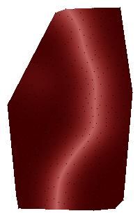
10
functions given e.g. in Figure 3b, d, f and once with the normalised empirical
covariance functions. The details of the used method and the results are given below.
As mentioned in the introduction, Rumpf et al. (2010) also performed a cluster
analysis to group dialect maps. The two major differences between their work and this
paper are the clustering method and the similarity measure. They use a hierarchical
clustering method, which implies that each map belongs to exactly one cluster. We use
a fuzzy clustering technique which gives a “weak” result. This means that each map
belongs to each cluster with a certain probability. Nevertheless, each map can be
assigned to the cluster with the highest membership probability which gives a “hard”
result as well. The second big difference between Rumpf et al. and our approach is how
similarity between maps is defined. The method presented here is based on the
empirical covariance function, as detailed in Section 3.2. This means that two maps are
similar if they share the same spatial structure, independent of the concrete locations. In
contrast to this, Rumpf et al. measure similarity with respect to the locations of spatial
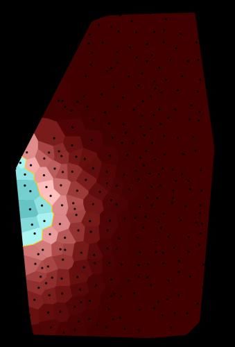
structures, i.e. two maps are similar if they are almost coincident. Figure 4 shows three
maps (displayed as area-class maps) to illustrate the different notions of similarity. With
the definition in Rumpf et al., the maps in Figure 4a and Figure 4b are similar, but the
map in Figure 4c is dissimilar to them because the green area has changed its location
considerably. However, in our setting, all three maps are similar because we ignore the
locations of the structures and consider only abstract spatial properties. This is an
advantage if one is interested in more universal, language internal patterns and
parameters of language change rather than distributions based on cultural phenomena
that are necessarily connected to specific locations (cities, political borders, trade routes
etc.).
(a) Area-class map (b) Area-class map (c) Area-class map
corresponding to the point- corresponding to the point- corresponding to the point-
symbol map 11107 Zecke symbol map 2084 flacken (“to symbol map 12066 Zinken der
(“tick”) slouch”) Heugabel (“teeth of the
pitchfork”)
Figure 4. Examples to illustrate different notions of similarity
There is a variety of algorithms to perform cluster analysis but they all have a crucial
point in common: how many clusters are naturally contained in a dataset? Or, in other
words, how do we choose the optimal number of clusters? If there are too few clusters,11
objects with quite different properties are classified as similar. On the other hand, if the
chosen number of clusters is too large, some natural clusters are split. We will follow
Goutte et al. (1999) and apply a two-stage strategy. First, we use a hierarchical
clustering method (Ward’s minimum variance method, see e.g. Ripley 2008 for an
introduction) and use the results to determine the optimal number of clusters in the data.
Therefore, we combine two of several known methods, the elbow criterion (see Goutte
et al. 1999) and the silhouettes (see Rousseeuw 1987). Both lead to the same results,
namely to use 7, 13 or 29 clusters if the sample variance is normalised to one and to use
6, 14 or 24 clusters otherwise. As it cannot be expected that the clusters are clearly
separated, we use the Fuzzy C-Means clustering technique (developed by Bezdek 1981)
to build the clusters in the second step. Its advantage is that a map is not assigned to
exactly one cluster but belongs to each cluster with a certain membership probability. 6
Finally, the map can be assigned to the cluster with the highest membership probability;
hence, we can define the centre of a cluster as the set of maps in the cluster with high
membership probability. Conversely, if there is no distinct maximal probability for a
specific map, this can be an indicator that the current map is an outlier. The following
chapter illustrates and analyses some basic results obtained by these methods.
4. Results
4.1 Overview of the results
We present the results of the cluster analysis for the case in which the variance is not
normalised. Otherwise the interpretation of the results is analogous. In either case, the
six volumes themselves show no strikingly clear distribution into separate clusters. This
is hardly surprising if one takes into account the wide semantic scope of each single
volume: while it is intuitively plausible to group the topics into volumes in the way
shown in Table 1, semantic differences between the grouped topics are pretty evident.
Still, even such a coarse criterion shows the emergence of overt tendencies. Figure 5
displays how many percent of a cluster originate from the same volume (visualised
through edge length of the squares). Distributions should not be overstated, but still they
are salient. The column far to the right (D) is not an actual cluster, but indicates the
default value for the average cluster; it is included for reasons of comparison.
Volume 13
Volume 12
Volume 11
Volume 10
Volume 8
Volume 2
Cluster 1 2 3 4 5 6 7 8 9 10 11 12 13 14 15 16 17 18 19 20 21 22 23 24 D
Figure 5. Distribution of the six SBS volumes on lexis into 24 clusters
If we use a finer semantic grid, i.e. if we use further categorisations, the results tend to
become increasingly distinct. Figure 6 visualises the inclusion of the 31 categories from
Table 1 (x-axis) into 24 clusters (y-axis); the warmer the colour, the higher the relative
amount of maps belonging to a certain category in a cluster.12 Figure 6. Nexus of 24 clusters and 31 categories 4.2 Validity of the results Prior to interpretation, one should bear two things in mind: first, some of these categories contain rather small numbers of maps. For example, category 10 (“must production (for beverages)”) includes merely three maps, category 11 (flowers) only four. Thus, high results for these categories might not be as meaningful as the visualisation suggests. To overcome these difficulties, we perform statistical tests to answer the question “Is the number of maps from a specific category in a given cluster significantly higher than the average?”. For most of the combinations of cluster and category which are marked with a yellow, orange or red square in Figure 6, this question can be affirmed at the significance level of 5%. However, the answer depends on the number of maps in the category as well as on the cluster size. Second, dividing a total sum of 736 maps into only 31 categories still is a quite coarse act (in respect to semantics); for a lot of maps, the affiliation to one or the other category seems rather arbitrary. Of course, this is a well-known problem of semantics that cannot be exhaustively discussed here (cf. for example Aitchison 2003). To further exemplify the practical value of the technique, we elaborate on the details of two different clusters, one seeming rather indifferent at first sight, the other showing more lucid results. The one with the clearer results will serve to illustrate the spatial similarities that the method is based on while the second will show how a closer investigation can reveal underlying semantic structures in a cluster.
13
4.3 First example: Structure and similarity
For a detailed view on the inner structure of the clusters, cluster 1 from Figure 6 was
chosen; as can be seen there, it shows elevated values for some categories (“habitation
and furnishing” (cat. 6), “adverbs” (cat. 17), “poultry keeping and beekeeping” (cat. 20)
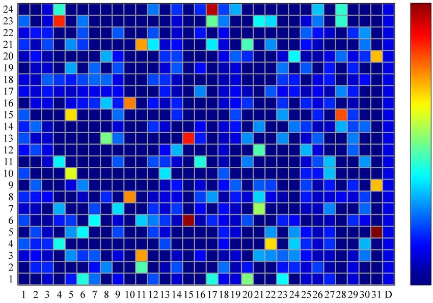
and “soil and cultivation” (cat. 23)). Its prevalence maps are displayed in Figure 7.
Figure 7. Spatial similarities of maps in cluster 1 from Figure 6
As mentioned in Section 3.3, for each map, the fuzzy clustering algorithm yields a value
that indicates how probable the map’s affiliation to a certain cluster is. Accordingly,
each cluster has an ideal value, a “centre”. The greater the distance of a map to this
(figurative) centre gets, the smaller is the probability that the map belongs to this cluster.
In Figure 7, the grade of probability is indicated by isolines. The maps close to the
centre of the figure have a high membership probability for this cluster and hence lie in
the cluster centre. Towards the outer boundary the affiliation to other clusters becomes
more and more likely. However, for all maps shown in Figure 6, the probability that the
map belongs to cluster 1 is higher than the membership probabilities for the other 23
clusters.
Visual similarity of the maps (i.e. similarity that is apparent to the eye) is roughly
indicated by radial proximity in Figure 7. This is an interpretation of the geographic
structure of the data, not the semantic one: which maps show spatial similarities? Note
for example the maps directly beneath the percentage bar: they share both a border that
roughly coincides with the Lech, the river separating the Swabian (west) and the
Bavarian (east) part of the area, and a border in the northeast. The maps on the upper
right edge of Figure 7 also feature the area in the northeast, but lack the Lech separation.14
The different constellations show that the spatial similarity of the maps is not limited to
the positions of the variants. The obvious reason for this is that the covariance is not
measured with respect to locations but only depends on distances (see Section 3.2). This
facilitates the detection of phenomena that would evade analysis if we merely
concentrated on maps that share records on the same locations (i.e. overlap to a certain
extent) or in the vicinity (as it is done in Grieve 2009, 2011 through means of spatial
autocorrelation). Moreover, the method also groups maps that show comparable
structures, but on different locations. For non-agglomerative clustering of single maps
based on the location of spatial structures, see Rumpf et al. (2010).
4.4 Second example: Semantic interpretation
Cluster number 12 from the set in Figure 6 serves as an example for possible semantic
interpretations: overall it does not show extremely salient distributions of the 31
categories. Nonetheless, this is not a flaw of our method, but rather of the categories
themselves. We deliberately chose this rather unimpressive looking cluster to
demonstrate that a closer analysis can reveal semantic relations between the maps that
were not indicated by the original categorisation.
Table 2. Content of cluster 12 from Figure 6
map vol. nr. % category
Wo läßt man die geformten Laibe nochmals
10 145 97,73 nutrition, cooking and baking
gehen? “Where are the loafs put to prove?”
Speichel rinnen lassen “to let saliva dribble” 2 43 97,61 physical and emotional expressions
hecheln vom Hund “dog’s panting ” 11 134 96,69 pets
Achsel “armpit” 2 20 93,39 the human body
Heurupfer
12 96 90,10 hay harvest
“tool for pulling hay out of haystacks”
Heuernte “haying” 12 54 88,42 hay harvest
Kipfen “lateral support of the chart” 13 75 77,13 transport
schleppend gehen “to scuffle, to shuffle” 2 76 66,51 physical and emotional expressions
gesammelte Getreidehaufen
12 112 58,19 crop
“stacked piles of grain”
Deichselarme/Hahl “towbars” 13 83 56,36 transport
Schupfnudeln
10 94 53,37 nutrition, cooking and baking
“finger-shaped potato dumplings”
Schicht auf dem Heuwagen
12 84 51,85 hay harvest
“layer on the hay chart”
kriechen “to crawl” 2 107 42,75 community
Wäsche spülen “to rinse” 10 37 40,95 household
Rückstand beim Buttereinsieden
10 77 36,25 nutrition, cooking and baking
“residue from simmering butter”
die Käserei “cheese dairy” 11 70 27,89 cattle and dairy processing
The value for “percentage” indicates the membership probability of the map to this
cluster. Again, lower values might indicate that a map is not clearly assigned to a
specific cluster but that the map’s phenomenon is subject to a more idiosyncratic type of
behaviour.
If we take Table 1 as point of reference, the four maps Speichel rinnen lassen (“to let
saliva dribble”), hecheln vom Hund (“dog’s panting”), schleppend gehen (“to scuffle, to
shuffle”) and kriechen (“to crawl”) all originate from different categories. But they15
share one concept that could approximately be paraphrased as “slow movement under
hindering circumstances”.
The category “hay harvest” already is most prominent in this single cluster, but by
combining two closely related categories, the results are even clearer: Kipfen (“lateral
support of the chart”) and Deichselarme/Hahl (“towbars”) are featured in the category
“transport”, but it is pretty evident that they are mandatory tools for harvesting.
These findings show that almost one third (“transport”/”hay harvest”) or one quarter
(“slow movement under hindering circumstances”), respectively, of the cluster’s maps
belong to the same semantic field (or to the same cognitive frame; cf. Aitchison 2003
and Vigliocco & Vinson 2009 for further reading on frames, fields and concepts).
Figure 8 visualises those semantic fields in cluster 12 (for reasons of visual clarity only
the English translations are given). The ovals represent the categories according to
Table 1 whereas the rectangles represent the single maps. Semantic similarities are
indicated by proximity: the frame-phenomena discussed above are located in the upper
and lower right corners.
Figure 8. Semantic contiguities in cluster 12 from Figure 6
The analysis of this cluster thus suggests that the domains of transport/hay harvest
and the abstract trait of slow motion share their spatial distribution of variants in the
area of the SBS.
As the nexus in Figure 6 shows, there are a number of clusters that – like cluster 12
– feature no significant preferences at first sight. Still, they can be interpreted (as we
have no reason to assume that any of the clusters are mere statistical artefacts). The
emerging connections between spatial structure and form provide the means for possible
new approaches to semantic theory and categorisation that could only be hinted at here.
This can serve as an important step towards a framework for what could be called
‘cognitive geolinguistics’ (reflecting desiderata uttered e.g. in Kristiansen & Dirven
2008 and Kristiansen 2008).
Findings like these are only possible if every step taken remains fully transparent, i.e.
if the constituents of groups of maps from the corpus are identifiable at any time. The
present combination of the particular benefits of quantitative dialectology and corpus
linguistics facilitates this a lot.16 5. Summary, conclusions and outlook After pre-processing the data, i.e. transforming the point-symbol maps of dialect atlases into prevalence maps, we measure the empirical covariance function for each map. It describes the spatial structure of a map independent of the actual positions of the structures. This enables the researcher to look for abstract rather than concrete patterns. Based on the empirical covariance function, we perform a two-stage cluster analysis where we first use a hierarchical clustering method to determine the most reasonable number of clusters and secondly employ the Fuzzy C-Means technique to cluster the corpus of maps into fuzzy groups. The advantage of building fuzzy groups is that this allows for defining the centre of a cluster in contrast to its periphery. As could be seen, this method has two different aspects: first, taking a geographical position, it becomes possible to group dialect maps with similar spatial properties. Second, it is useful for linguistic categorisation by showing which maps (i.e. which linguistic variables) share spatial features. We could show that complex interpretations can already be drawn from lexical data. Given the sometimes erratic nature of lexical diffusion, we hypothesise that phonetics and morphology will show clearer, more uniform patterns of spatial structures than lexis, which we thus see as an experimentum crucis: if the techniques work on lexis, we suppose they work on phonetics and morphology as well. Furthermore, statistical-based techniques like these for the first time provide the opportunity to treat the central contents of dialect atlases – the maps – as a corpus that is fully accessible through automated processes. This provides a new angle on corpus dialectology, which until now had been constrained by issues of using categorical data as well as the lack of spatial pattern detection when it came to dealing with the contents of dialect atlases. Notes * The authors’ work is supported by the DFG research project “Neue Dialektometrie mit Methoden der stochastischen Bildanalyse” (“New Dialectometry using Methods from Stochastic Image Analysis”) of the Chair of German Linguistics at the University of Augsburg and the Institute of Stochastics at the University of Ulm; see http://www.uni-ulm.de/en/mawi/institute-of- stochastics/research/projekte/linguistic-atlas.html. In addition to the editors and the reviewers of this paper, we would like to thank S. Elspaß, W. König, V. Schmidt and E. Spodarev for fruitful discussions and helpful comments. 1. Older approaches to examine the spatiality of semantics in a quantitative way exist (cf. e.g. Baka & Chauveau 1981); however, they are based on multivariate statistical analyses of categorical data, not fuzzy clustering of continuous data. This makes them less compatible with corpus linguistics as well as unable to detect spatial structures independently of their concrete positions. This also marks a clear difference to the spatial autocorrelation techniques recently introduced to dialectology by Grieve (2009, 2011). 2. See SBS vol. 1, p. 16f. for further information on the choice of record locations. 3. The large amount of topics dealing with agricultural themes is due to (a) the area being rural for the most part and (b) the deliberate focus on traditional forms and variants. 4. In this paper, we utilise Euclidean space as a measure of distance. Other types of distance (like linguistic distance or travel time, cf. Gooskens 2005, Szmrecsanyi 2011) obviously are applicable as well.
17

5. Note that         is a special case; if we measure the covariance at a distance of zero kilometres, the
formula yields the variance of the measurement points.

6. This “fuzzy” approach also minimises the common risks of hierarchical clustering as outlined and
examined e.g. by Prokić & Nerbonne (2008), especially the high sensibility of the results to small nuances
in the data.

References

Adolphs, S., Knight, D. & Carter, R. 2011. “Capturing context for heterogeneous corpus
   analysis. Some first steps.” International Journal of Corpus Linguistics, 16 (3), 305–
   324.
Aitchison, J. 2003. Words in the Mind: An Introduction to the Mental Lexicon. 3rd
   edition. Malden, MA.: Blackwell Publishers.
Andersen, G. 2010. “How to use corpus linguistics in sociolinguistics.” In A. O’Keeffe
   & M. McCarthy (eds.), The Routledge Handbook of Corpus Linguistics. London,
   New York: Taylor & Francis, 547–562.
Anderwald, L. & Szmrecsanyi, B. 2009. “Corpus linguistics and dialectology.” In A.
   Lüdeling, M. Kytö & T. McEnery (eds.), Corpus Linguistics. An International
   Handbook. Handbücher zur Sprach- und Kommunikationswissenschaft (HSK) 29.2.
   Berlin, New York: de Gruyter, 1126–1140.
Baka, M. & Chauveau, J-P. 1981. “L’atlas linguistique et ethnographique de la Bretagne
   romane, de l’Anjou et du Maine.” In J-P. Benzécri (ed.), Pratique de l'analyse des
   données, tome 3. Linguistique et lexicologie. Paris: Dunod, 334–359.
Bezdek, J. 1981. Pattern Recognition with Fuzzy Objective Function Algorithms. New
   York: Plenum Press.
Britain, D. (2002). “Space and spatial diffusion.” In J. K. Chambers, P. Trudgill & N.
   Schilling-Estes (eds.), The Handbook of Language Variation and Change. Malden:
   Blackwell, 603–637.
Elspaß, S. 2007. “‘Everyday language’ in emigrant letters and its implications for
   language historiography – the German case.” Multilingua, 26 (2-3), 151–165.
Flowerdew, L. 2004. “The argument for using English specialized corpora to
   understand academic and professional settings.” In U. Connor & T. Upton (eds.),
   Discourse in the Professions: Perspectives from Corpus Linguistics. Amsterdam:
   John Benjamins, 11–33.
Goebl, H. 2006. “Recent advances in Salzburg dialectometry.” Literary and Linguistic
   Computing, 21 (4) [Special Issue on Progress in Dialectometry], 411–435.
Gooskens, Ch. 2005. “Traveling time as a predictor of linguistic distance.”
   Dialectologia et Geolinguistica, 13, 38–62.
Gordon, M. J. (2002). “Investigating chain shifts and mergers.” In J. K. Chambers, P.
   Trudgill & N. Schilling-Estes (eds.), The Handbook of Language Variation and
   Change. Malden: Blackwell, 244–266.
Goutte, C., Toft, P., Rostrup, E., Nielsen, F. & Hansen, L. 1999. “On clustering fMRI
   time series.” NeuroImage, 9, 298–310.
Gregory, I. N. & Hardie, A. 2011. “Visual GISting: Bringing together corpus linguistics
   and Geographical Information Systems.” Literary and Linguistic Computing, 26 (3),
   297–314.
Grieve, J. 2009. A Corpus-Based Regional Dialect Survey of Grammatical Variation in
   Written Standard American English. Ph.D. thesis, Northern Arizona University.
18

Grieve, J. 2011. “A regional analysis of contraction rate in written Standard American
   English.” International Journal of Corpus Linguistics, 16 (4), 514–546.
Haag, C. 1898. Die Mundarten des oberen Neckar- und Donaulandes. Schwäbisch-
   alemannisches Grenzgebiet: Baarmundarten. Reutlingen: Hutzler.
Händler, H. & Wiegand, H. E. 1982. “Das Konzept der Isoglosse: Methodische und
   terminologische Probleme.” In W. Besch, U. Knoop, W. Putschke & H. E. Wiegand
   (eds.), Dialektologie. Ein Handbuch zur deutschen und allgemeinen
   Dialektforschung. Berlin, New York: de Gruyter, 501–527.
Heeringa, W. 2004. Measuring Dialect Pronunciation Differences using Levenshtein
   Distance. Ph.D. thesis, Rijksuniversiteit Groningen.
Koester, A. 2010. “Building small specialised corpora.” In A. O’Keeffe & M. McCarthy
   (eds.), The Routledge Handbook of Corpus Linguistics. London, New York: Taylor
   & Francis, 66–79.
König, W. 1989. Die Aussprache des Schriftdeutschen in der Bundesrepublik
   Deutschland. Ismaning: Huber.
Kristiansen, G. 2008. “Style-shifting and shifting styles: A socio-cognitive approach to
   lectal variation.” In G. Kristiansen & R. Dirven (eds.), Cognitive Sociolinguistics.
   Berlin, New York: de Gruyter, 45–88.
Kristiansen, G. & Dirven, R. 2008. “Cognitive sociolinguistics: Rationale, methods and
   scope.” In G. Kristiansen & R. Dirven (eds.), Cognitive Sociolinguistics. Berlin, New
   York: de Gruyter, 1–17.
Naumann, C. L. 1982. “Kartographische Datendarstellung.” In W. Besch, U. Knoop, W.
   Putschke & H. E. Wiegand (eds.), Dialektologie. Ein Handbuch zur deutschen und
   allgemeinen Dialektforschung. Berlin, New York: de Gruyter, 667–692.
Nerbonne, J. & Kretzschmar, W. 2003. “Introducing computational methods in
   dialectometry.” Computers and the Humanities, 37 (3), 245–255.
Nerbonne, J. 2009. “Data-driven dialectology.” Language and Linguistics Compass, 3
   (1), 175–198.
Prokić, J. & Nerbonne, J. 2008. “Recognising groups among dialects.” International
   Journal of Humanities and Arts Computing, 2 (1–2), 153–172.
Ripley, B. 2008. Pattern Recognition and Neural Networks. Cambridge: Cambridge
   University Press.
Rousseeuw, P. 1987. “Silhouettes: A graphical aid to the interpretation and validation of
   cluster analysis.” Journal of Computational and Applied Mathematics, 20, 53–65.
Rumpf, J., Pickl, S., Elspaß, S., König, W. & Schmidt, V. 2009. “Structural analysis of
   dialect maps using methods from spatial statistics.” Zeitschrift für Dialektologie und
   Linguistik, 76 (3), 280–308.
Rumpf, J., Pickl, S., Elspaß, S., König, W. & Schmidt, V. 2010. “Quantification and
   statistical analysis of structural similarities in dialectological area-class maps.“
   Dialectologia et Geolinguistica, 18, 73–100.
Sachs, L. 2003. Angewandte Statistik: Anwendung statistischer Methoden. Berlin:
   Springer.
SBS = König, W. (ed.) 1996-2009. Sprachatlas von Bayerisch-Schwaben. [Volumes
   1-14] Heidelberg: Winter.
Szmrecsanyi, B. 2008. “Corpus-based dialectometry: Aggregate morphosyntactic
   variability in British English dialects.” International Journal of Humanities and Arts
   Computing, 2 (1–2), 279–296.
19

Szmrecsanyi, B. 2011. “Corpus-based dialectometry: a methodological sketch.”
  Corpora, 6 (1), 45–76.
Teuchert, H. 1924. “Lautschrift des Teuthonista.” Teuthonista, 1, 5.
Vigliocco, G. & Vinson, D. P. 2009. “Semantic representation.” In M. G. Gaskell (ed.),
  The Oxford Handbook of Psycholinguistics. Oxford: Oxford University Press, 195–
  215.
Wackernagel, H. 1998. Multivariate Geostatistics. Berlin: Springer.
Wiesinger, P. 1982. “Die Reihenschrittheorie: Muster eines dialektologischen Beitrags
  zur Erklärung des Lautwandels.” In W. Besch, U. Knoop, W. Putschke & H. E.
  Wiegand (eds.), Dialektologie. Ein Handbuch zur deutschen und allgemeinen
  Dialektforschung. Berlin, New York: de Gruyter, 144–151.

Authors’ addresses

Daniel Meschenmoser                        Simon Pröll
University of Ulm                          University of Augsburg
Institute of Stochastics                   Deutsche Sprachwissenschaft
Helmholtzstr. 18                           Universitätsstr. 10
89069 Ulm                                  86159 Augsburg
Germany                                    Germany

d.meschenmoser@gmail.com                   simon.proell@phil.uni-augsburg.de
You can also read