Improved Techniques for Grid Mapping with Rao-Blackwellized Particle Filters
←
→
Page content transcription
If your browser does not render page correctly, please read the page content below
1

                        Improved Techniques for Grid Mapping
                        with Rao-Blackwellized Particle Filters
                            Giorgio Grisetti∗†          Cyrill Stachniss‡∗          Wolfram Burgard∗
   ∗   University of Freiburg, Dept. of Computer Science, Georges-Köhler-Allee 79, D-79110 Freiburg, Germany
   †   Dipartimento Informatica e Sistemistica, Universitá “La Sapienza”, Via Salaria 113, I-00198 Rome, Italy
            ‡ Eidgenössische Technische Hochschule Zurich (ETH), IRIS, ASL, 8092 Zurich, Switzerland

    Abstract— Recently, Rao-Blackwellized particle filters have        •   An adaptive resampling technique which maintains a
been introduced as an effective means to solve the simultaneous            reasonable variety of particles and in this way enables
localization and mapping problem. This approach uses a particle            the algorithm to learn an accurate map while reducing
filter in which each particle carries an individual map of the
environment. Accordingly, a key question is how to reduce the              the risk of particle depletion.
number of particles. In this paper, we present adaptive techniques   The proposal distribution is computed by evaluating the like-
for reducing this number in a Rao-Blackwellized particle filter      lihood around a particle-dependent most likely pose obtained
for learning grid maps. We propose an approach to compute
                                                                     by a scan-matching procedure combined with odometry in-
an accurate proposal distribution taking into account not only
the movement of the robot but also the most recent observation.      formation. In this way, the most recent sensor observation is
This drastically decreases the uncertainty about the robot’s pose    taken into account for creating the next generation of particles.
in the prediction step of the filter. Furthermore, we present an     This allows us to estimate the state of the robot according to
approach to selectively carry out resampling operations which        a more informed (and thus more accurate) model than the
seriously reduces the problem of particle depletion. Experimental
                                                                     one obtained based only on the odometry information. The
results carried out with real mobile robots in large-scale indoor
as well as in outdoor environments illustrate the advantages of      use of this refined model has two effects. The map is more
our methods over previous approaches.                                accurate since the current observation is incorporated into the
   Index Terms— SLAM, Rao-Blackwellized particle filter, adap-
                                                                     individual maps after considering its effect on the pose of
tive resampling, motion-model, improved proposal                     the robot. This significantly reduces the estimation error so
                                                                     that less particles are required to represent the posterior. The
                                                                     second approach, the adaptive resampling strategy, allows us
                       I. I NTRODUCTION
                                                                     to perform a resampling step only when needed and in this
   Building maps is one of the fundamental tasks of mobile           way keeping a reasonable particle diversity. This results in a
robots. In the literature, the mobile robot mapping problem is       significantly reduced risk of particle depletion.
often referred to as the simultaneous localization and mapping          The work presented in this paper is an extension of our
(SLAM) problem [4, 6, 9, 15, 16, 26, 29, 32, 39]. It is              previous work [14] as it further optimizes the proposal dis-
considered to be a complex problem, because for localization         tribution to even more accurately draw the next generation
a robot needs a consistent map and for acquiring a map a             of particles. Furthermore, we added a complexity analysis, a
robot requires a good estimate of its location. This mutual          formal description of the used techniques, and provide more
dependency between the pose and the map estimates makes              detailed experiments in this paper. Our approach has been
the SLAM problem hard and requires searching for a solution          validated by a set of systematic experiments in large-scale
in a high-dimensional space.                                         indoor and outdoor environments. In all experiments, our
   Murphy, Doucet, and colleagues [6, 32] introduced Rao-            approach generated highly accurate metric maps. Additionally,
Blackwellized particle filters as an effective means to solve        the number of the required particles is one order of magnitude
the simultaneous localization and mapping problem. The main          lower than with previous approaches.
problem of the Rao-Blackwellized approaches is their com-               This paper is organized as follows. After explaining how a
plexity measured in terms of the number of particles required        Rao-Blackwellized filter can be used in general to solve the
to build an accurate map. Therefore, reducing this quantity          SLAM problem, we describe our approach in Section III. We
is one of the major challenges for this family of algorithms.        then provide implementation details in Section IV. Experi-
Additionally, the resampling step can potentially eliminate          ments carried out on real robots are presented in Section VI.
the correct particle. This effect is also known as the particle      Finally, Section VII discusses related approaches.
depletion problem or as particle impoverishment [44].
   In this work, we present two approaches to substantially
increase the performance of Rao-Blackwellized particle filters          II. M APPING   WITH   R AO -B LACKWELLIZED PARTICLE
applied to solve the SLAM problem with grid maps:                                                F ILTERS
   • A proposal distribution that considers the accuracy of the        According to Murphy [32], the key idea of the Rao-
     robot’s sensors and allows us to draw particles in a highly     Blackwellized particle filter for SLAM is to estimate the joint
     accurate manner.                                                posterior p(x1:t , m | z1:t , u1:t−1 ) about the map m and the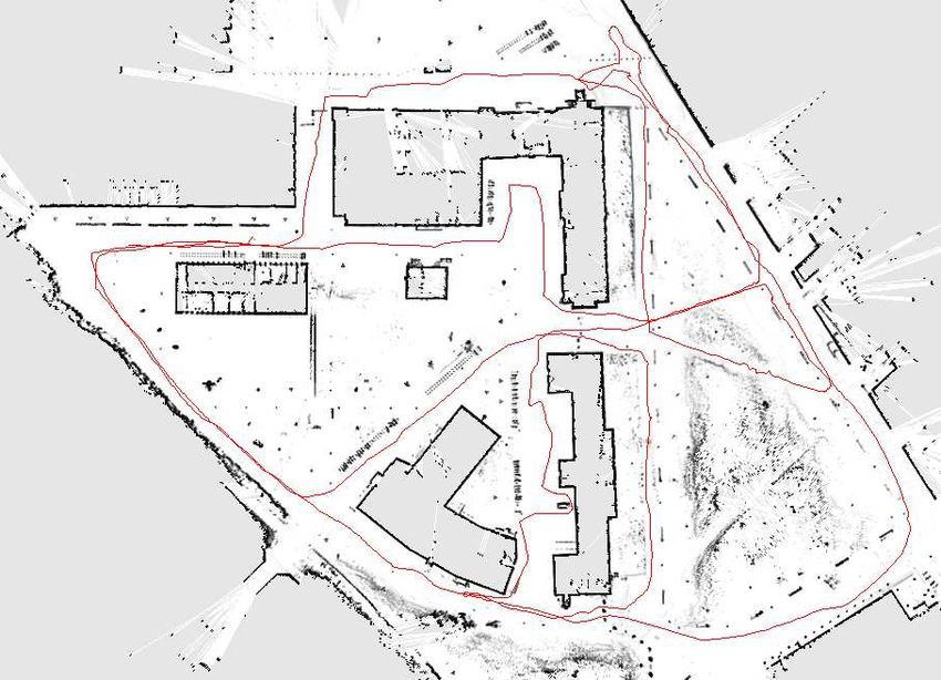
2

trajectory x1:t = x1 , . . . , xt of the robot. This estimation is     increases over time, this procedure would lead to an obviously
performed given the observations z1:t = z1 , . . . , zt and the        inefficient algorithm. According to Doucet et al. [7], we obtain
odometry measurements u1:t−1 = u1 , . . . , ut−1 obtained by           a recursive formulation to compute the importance weights by
the mobile robot. The Rao-Blackwellized particle filter for            restricting the proposal π to fulfill the following assumption
SLAM makes use of the following factorization
                                                                           π(x1:t | z1:t , u1:t−1 )        = π(xt | x1:t−1 , z1:t , u1:t−1 )
          p(x1:t , m | z1:t , u1:t−1 ) =                                                                           ·π(x1:t−1 | z1:t−1 , u1:t−2 ). (3)
               p(m | x1:t , z1:t ) · p(x1:t | z1:t , u1:t−1 ).   (1)
                                                                       Based on Eq. (2) and (3), the weights are computed as
This factorization allows us to first estimate only the trajectory                           (i)
of the robot and then to compute the map given that trajectory.            (i)        p(x1:t | z1:t , u1:t−1 )
                                                                         wt      =           (i)
                                                                                                                                                      (4)
Since the map strongly depends on the pose estimate of                                π(x1:t | z1:t , u1:t−1 )
the robot, this approach offers an efficient computation. This                                      (i)                  (i)     (i)
                                                                                      ηp(zt | x1:t , z1:t−1 )p(xt | xt−1 , ut−1 )
technique is often referred to as Rao-Blackwellization.                          =                   (i)         (i)
   Typically, Eq. (1) can be calculated efficiently since the pos-                             π(xt | x1:t−1 , z1:t , u1:t−1 )
terior over maps p(m | x1:t , z1:t ) can be computed analytically                             (i)
                                                                                          p(x1:t−1 | z1:t−1 , u1:t−2 )
using “mapping with known poses” [31] since x1:t and z1:t                             ·       (i)
                                                                                                                                                      (5)
are known.                                                                                π(x1:t−1 | z1:t−1 , u1:t−2 )
                                                                                          |           {z             }
   To estimate the posterior p(x1:t | z1:t , u1:t−1 ) over the po-                                         (i)
                                                                                                          wt−1
tential trajectories, one can apply a particle filter. Each particle                                (i)      (i)       (i)     (i)
represents a potential trajectory of the robot. Furthermore, an                       p(zt | mt−1 , xt )p(xt | xt−1 , ut−1 )                    (i)
                                                                                 ∝                          (i)
                                                                                                                                             · wt−1 .(6)
individual map is associated with each sample. The maps are                                    π(xt |      x1:t−1 , z1:t , u1:t−1 )
built from the observations and the trajectory represented by
the corresponding particle.                                            Here η = 1/p(zt | z1:t−1 , u1:t−1 ) is a normalization factor
   One of the most common particle filtering algorithms is             resulting from Bayes’ rule that is equal for all particles.
the sampling importance resampling (SIR) filter. A Rao-                   Most of the existing particle filter applications rely on the
Blackwellized SIR filter for mapping incrementally processes           recursive structure of Eq. (6). Whereas the generic algorithm
the sensor observations and the odometry readings as they              specifies a framework that can be used for learning maps, it
are available. It updates the set of samples that represents the       leaves open how the proposal distribution should be computed
posterior about the map and the trajectory of the vehicle. The         and when the resampling step should be carried out. Through-
process can be summarized by the following four steps:                 out the remainder of this paper, we describe a technique that
                                                         (i)           computes an accurate proposal distribution and that adaptively
   1) Sampling: The next generation of particles {xt } is ob-
                                       (i)                             performs resampling.
       tained from the generation {xt−1 } by sampling from the
       proposal distribution π. Often, a probabilistic odometry
       motion model is used as the proposal distribution.               III. RBPF    WITH I MPROVED         P ROPOSALS               AND   A DAPTIVE
   2) Importance Weighting: An individual importance weight                                           R ESAMPLING
         (i)                                                             In the literature, several methods for computing improved
       wt is assigned to each particle according to the impor-
       tance sampling principle                                        proposal distributions and for reducing the risk of particle
                                   (i)                                 depletion have been proposed [7, 30, 35]. Our approach applies
                       (i)     p(x1:t | z1:t , u1:t−1 )                two concepts that have previously been identified as key
                     wt =          (i)
                                                          .      (2)
                              π(x1:t | z1:t , u1:t−1 )                 pre-requisites for efficient particle filter implementations (see
      The weights account for the fact that the proposal distri-       Doucet et al. [7]), namely the computation of an improved
      bution π is in general not equal to the target distribution      proposal distribution and an adaptive resampling technique.
      of successor states.
  3) Resampling: Particles are drawn with replacement pro-             A. On the Improved Proposal Distribution
      portional to their importance weight. This step is nec-             As described in Section II, one needs to draw samples from
      essary since only a finite number of particles is used to        a proposal distribution π in the prediction step in order to ob-
      approximate a continuous distribution. Furthermore, re-          tain the next generation of particles. Intuitively, the better the
      sampling allows us to apply a particle filter in situations      proposal distribution approximates the target distribution, the
      in which the target distribution differs from the proposal.      better is the performance of the filter. For instance, if we were
      After resampling, all the particles have the same weight.        able to directly draw samples from the target distribution, the
  4) Map Estimation: For each particle, the corresponding              importance weights would become equal for all particles and
                                 (i)
      map estimate p(m(i) | x1:t , z1:t ) is computed based on         the resampling step would no longer be needed. Unfortunately,
                       (i)
      the trajectory x1:t of that sample and the history of            in the context of SLAM a closed form of this posterior is not
      observations z1:t .                                              available in general.
  The implementation of this schema requires to evaluate                  As a result, typical particle filter applications [3, 29] use
the weights of the trajectories from scratch whenever a new            the odometry motion model as the proposal distribution. This
observation is available. Since the length of the trajectory           motion model has the advantage that it is easy to compute for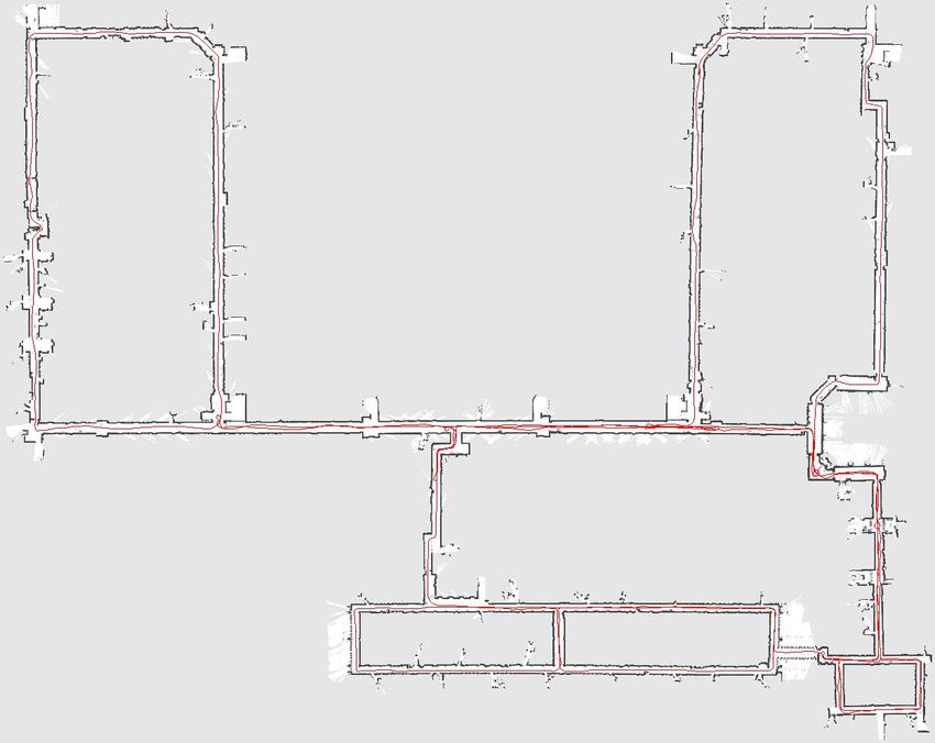
3
of the weights turns into
p(z|x)
p(x|x’,u) (i) (i) (i) (i)
(i) (i) ηp(zt | mt−1 , xt )p(xt | xt−1 , ut−1 )
wt = wt−1 (i) (i)
(10)
likelihood
p(xt | mt−1 , xt−1 , zt , ut−1 )
(i) (i) (i) (i)
(i) p(zt | mt−1 , xt )p(xt | xt−1 , ut−1 )
∝ wt−1 (i) (i)
(11)
p(zt |mt−1 ,xt )p(xt |xt−1 ,ut−1 )
(i) (i)
p(zt |mt−1 ,xt−1 ,ut−1 )
|{z} (i) (i) (i)
L(i) robot position = wt−1 · p(zt | mt−1 , xt−1 , ut−1 ) (12)
Z
(i) (i)
Fig. 1. The two components of the motion model. Within the interval L(i)
= wt−1 · p(zt | x′ )p(x′ | xt−1 , ut−1 ) dx′ . (13)
the product of both functions is dominated by the observation likelihood in
case an accurate sensor is used. When modeling a mobile robot equipped with an accurate
sensor like, e.g., a laser range finder, it is convenient to use
such an improved proposal since the accuracy of the laser
most types of robots. Furthermore, the importance weights range finder leads to extremely peaked likelihood functions.
are then computed according to the observation model p(zt | In the context of landmark-based SLAM, Montemerlo et
m, xt ). This becomes clear by replacing π in Eq. (6) by the al. [26] presented a Rao-Blackwellized particle filter that uses
motion model p(xt | xt−1 , ut−1 ) a Gaussian approximation of the improved proposal. This
Gaussian is computed for each particle using a Kalman filter
(i) (i) (i) (i)
(i) (i) ηp(zt | mt−1 , xt )p(xt | xt−1 , ut−1 ) that estimates the pose of the robot. This approach can be used
wt = wt−1 (i) (i)
(7) when the map is represented by a set of features and if the
p(xt | xt−1 , ut−1 )
(i) (i) (i)
error affecting the feature detection is assumed to be Gaussian.
∝ wt−1 · p(zt |mt−1 , xt ). (8) In this work, we transfer the idea of computing an improved
proposal to the situation in which dense grid maps are used
This proposal distribution, however, is suboptimal especially instead of landmark-based representations.
when the sensor information is significantly more precise than
the motion estimate of the robot based on the odometry, B. Efficient Computation of the Improved Proposal
which is typically the case if a robot equipped with a laser When modeling the environment with grid maps, a closed
range finder (e.g., with a SICK LMS). Figure 1 illustrates form approximation of an informed proposal is not directly
a situation in which the meaningful area of the observation available due to the unpredictable shape of the observation
likelihood is substantially smaller than the meaningful area of likelihood function.
the motion model. When using the odometry model as the In theory, an approximated form of the informed proposal
proposal distribution in such a case, the importance weights can be obtained using the adapted particle filter [35]. In this
of the individual samples can differ significantly from each framework, the proposal for each particle is constructed by
other since only a fraction of the drawn samples cover the computing a sampled estimate of the optimal proposal given
regions of state space that have a high likelihood under the in Eq. (9). In the SLAM context, one would first have to
observation model (area L(i) in Figure 1). As a result, one sample a set of potential poses xj of the robot from the motion
needs a comparably high number of samples to sufficiently (i)
model p(xt | xt−1 , ut−1 ). In a second step, these samples
cover the regions with high observation likelihood. need to be weighed by the observation likelihood to obtain
A common approach – especially in localization – is to use an approximation of the optimal proposal. However, if the
a smoothed likelihood function, which avoids that particles observation likelihood is peaked the number of pose samples
close to the meaningful area get a too low importance weight. xj that has to be sampled from the motion model is high,
However, this approach discards useful information gathered since a dense sampling is needed for sufficiently capturing
by the sensor and, at least to our experience, often leads to the typically small areas of high likelihood. This results in a
less accurate maps in the SLAM context. similar problem than using the motion model as the proposal:
To overcome this problem, one can consider the most recent a high number of samples is needed to sufficiently cover the
sensor observation zt when generating the next generation of meaningful region of the distribution.
samples. By integrating zt into the proposal one can focus One of our observations is that in the majority of cases
the sampling on the meaningful regions of the observation the target distribution has only a limited number of maxima
likelihood. According to Doucet [5], the distribution and it mostly has only a single one. This allows us to sample
positions xj covering only the area surrounding these maxima.
(i) (i)
p(xt | mt−1 , xt−1 , zt , ut−1 ) = Ignoring the less meaningful regions of the distribution saves a
(i) (i) significant amount of computational resources since it requires
p(zt | mt−1 , xt )p(xt | xt−1 , ut−1 )
(9) less samples. In the previous version of this work [14], we
(i) (i) (i)
p(zt | mt−1 , xt−1 , ut−1 ) approximated p(xt | xt−1 , ut−1 ) by a constant k within the
interval L(i) (see also Figure 1) given by
is the optimal proposal distribution with respect to the variance n
(i)
o
of the particle weights. Using that proposal, the computation L(i) = x p(zt | mt−1 , x) > ǫ . (14)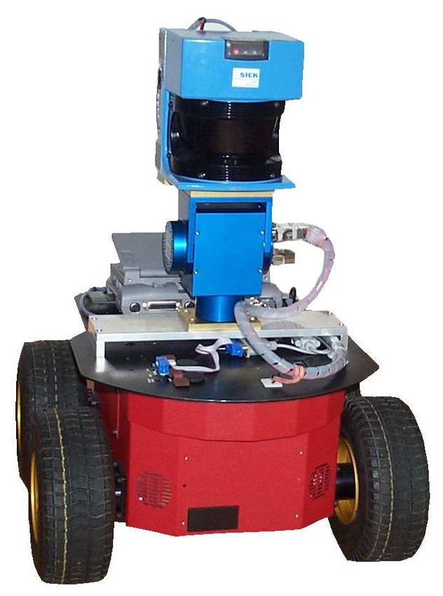
4

                                                                                                   (i)
                                                                                             =   wt−1 · η (i) .                                   (19)

                                                                                     Note that η (i) is the same normalization factor that is used in
                                                                                     the computation of the Gaussian approximation of the proposal
                                                                                     in Eq. (17).

                                                                                     C. Discussion about the Improved Proposal
 (a)                           (b)                              (c)
                                                                                        The computations presented in this section enable us to
Fig. 2. Particle distributions typically observed during mapping. In an open         determine the parameters of a Gaussian proposal distribution
corridor, the particles distribute along the corridor (a). In a dead end corridor,   for each particle individually. The proposal takes into account
the uncertainty is small in all dimensions (b). Such posteriors are obtained         the most recent odometry reading and laser observation while
because we explicitely take into account the most recent observation when
sampling the next generation of particles. In contrast to that, the raw odometry     at the same time allowing us efficient sampling. The resulting
motion model leads less peaked posteriors (c).                                       densities have a much lower uncertainty compared to situations
                                                                                     in which the odometry motion model is used. To illustrate this
                                                                                     fact, Figure 2 depicts typical particle distributions obtained
In our current approach, we consider both components, the                            with our approach. In case of a straight featureless corridor,
observation likelihood and the motion model within that                              the samples are typically spread along the main direction of
interval L(i) . We locally approximate the posterior p(xt |                          the corridor as depicted in Figure 2 (a). Figure 2 (b) illustrates
  (i)    (i)
mt−1 , xt−1 , zt , ut−1 ) around the maximum of the likelihood                       the robot reaching the end of such a corridor. As can be seen,
function reported by a scan registration procedure.                                  the uncertainty in the direction of the corridor decreases and all
   To efficiently draw the next generation of samples, we                            samples are centered around a single point. In contrast to that,
compute a Gaussian approximation N based on that data.                               Figure 2 (c) shows the resulting distribution when sampling
The main differences to previous approaches is that we first                         from the raw motion model.
use a scan-matcher to determine the meaningful area of                                  As explained above, we use a scan-matcher to determine
the observation likelihood function. We then sample in that                          the mode of the meaningful area of the observation likelihood
meaningful area and evaluate the sampled points based on                             function. In this way, we focus the sampling on the important
                                                              (i)
the target distribution. For each particle i, the parameters µt                      regions. Most existing scan-matching algorithms maximize the
       (i)
and Σt are determined individually for K sampled points                              observation likelihood given a map and an initial guess of the
{xj } in the interval L(i) . We furthermore take into account                        robot’s pose. When the likelihood function is multi-modal,
the odometry information when computing the mean µ(i) and                            which can occur when, e.g., closing a loop, the scan-matcher
the variance Σ(i) . We estimate the Gaussian parameters as                           returns for each particle the maximum which is closest to the
                                      K                                              initial guess. In general, it can happen that additional maxima
               (i)              1 X                   (i)                            in the likelihood function are missed since only a single mode
              µt         =          ·    xj · p(zt | mt−1 , xj )
                               η (i) j=1                                             is reported. However, since we perform frequent filter updates
                                              (i)                                    (after each movement of 0.5 m or a rotation of 25◦ ) and
                              ·p(xj | xt−1 , ut−1 )                         (15)
                                                                                     limit the search area of the scan-matcher, we consider that the
                                       K
               (i)              1      X         (i)                                 distribution has only a single mode when sampling data points
              Σt         =          ·    p(zt | mt−1 , xj )
                               η (i) j=1                                             to compute the Gaussian proposal. Note that in situations like a
                                              (i)
                                                                                     loop closure, the filter is still able to keep multiple hypotheses
                              ·p(xj | xt−1 , ut−1 )                                  because the initial guess for the starting position of the scan-
                                              (i)         (i)                        matcher when reentering a loop is different for each particle.
                              ·(xj − µt )(xj − µt )T                        (16)
                                                                                        Nevertheless, there are situations in which the filter can – at
with the normalization factor
                                                                                     least in theory – become overly confident. This might happen
              X K
                            (i)                 (i)                                  in extremely cluttered environments and when the odometry
     η (i) =       p(zt | mt−1 , xj ) · p(xj | xt−1 , ut−1 ). (17)
                                                                                     is highly affected by noise. A solution to this problem is to
                     j=1
                                                                                     track the multiple modes of the scan-matcher and repeat the
In this way, we obtain a closed form approximation of the                            sampling process separately for each node. However, in our
optimal proposal which enables us to efficiently obtain the                          experiments carried out using real robots we never encountered
next generation of particles. Using this proposal distribution,                      such a situation.
the weights can be computed as
                                                                                        During filtering, it can happen that the scan-matching
   (i)             (i)                  (i)         (i)
 wt       =    wt−1 · p(zt | mt−1 , xt−1 , ut−1 )              (18)                  process fails because of poor observations or a too small
                      Z
                (i)              (i)               (i)                               overlapping area between the current scan and the previously
          =    wt−1 · p(zt | mt−1 , x′ ) · p(x′ | xt−1 , ut−1 ) dx                   computed map. In this case, the raw motion model of the
                             K
                             X                                                       robot which is illustrated in Figure 2 (c) is used as a proposal.
                (i)                             (i)                   (i)            Note that such situations occur rarely in real datasets (see also
          ≃    wt−1      ·         p(zt | mt−1 , xj ) · p(xj | xt−1 , ut−1 )
                             j=1                                                     Section VI-E).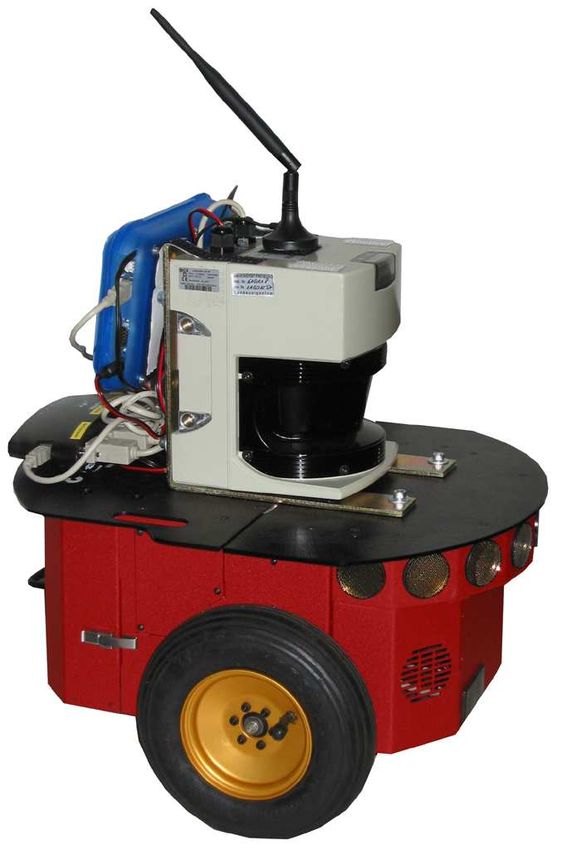
5

                                                                                                        (i)                 (i)
D. Adaptive Resampling                                                     target distribution p(zt | mt−1 , xj )p(xj | xt−1 , ut−1 ) in
   A further aspect that has a major influence on the per-                 the sampled positions xj . During this phase, also the
formance of a particle filter is the resampling step. During               weighting factor η (i) is computed according to Eq. (17).
                                                                                              (i)
resampling, particles with a low importance weight w(i) are             4) The new pose xt of the particle i is drawn from the
                                                                                                          (i)    (i)
typically replaced by samples with a high weight. On the one               Gaussian approximation N (µt , Σt ) of the improved
hand, resampling is necessary since only a finite number of                proposal distribution.
particles are used to approximate the target distribution. On           5) Update of the importance weights.
the other hand, the resampling step can remove good samples             6) The map m(i) of particle i is updated according to the
                                                                                          (i)
from the filter which can lead to particle impoverishment.                 drawn pose xt and the observation zt .
Accordingly, it is important to find a criterion for deciding        After computing the next generation of samples, a resampling
when to perform the resampling step. Liu [23] introduced the         step is carried out depending on the value of Neff .
so-called effective sample size to estimate how well the current
particle set represents the target posterior. In this work, we                        IV. I MPLEMENTATION I SSUES
compute this quantity according to the formulation of Doucet
                                                                        This section provides additional information about imple-
et al. [7] as
                                    1                                mentation details used in our current system. These issues are
                     Neff = PN             ,               (20)     not required for the understanding of the general approach but
                                       (i) 2
                               i=1 w̃                                complete the precise description of our mapping system. In
where w̃(i) refers to the normalized weight of particle i.           the following, we briefly explain the used scan-matching ap-
   The intuition behind Neff is as follows. If the samples were      proach, the observation model, and how to pointwise evaluate
drawn from the target distribution, their importance weights         the motion model.
would be equal to each other due to the importance sampling             Our approach applies a scan-matching technique on a per
principle. The worse the approximation of the target distri-         particle basis. In general, an arbitrary scan-matching technique
bution, the higher is the variance of the importance weights.        can be used. In our implementation, we use the scan-matcher
Since Neff can be regarded as a measure of the dispersion            “vasco” which is part of the Carnegie Mellon Robot Naviga-
of the importance weights, it is a useful measure to evaluate        tion Toolkit (CARMEN) [27, 36]. This scan-matcher aims to
how well the particle set approximates the target posterior.         find the most likely pose by matching the current observation
Our algorithm follows the approach proposed by Doucet et             against the map constructed so far
al. [7] to determine whether or not the resampling step should                       (i)                      (i)    ′(i)
                                                                                    x̂t = argmax p(x | mt−1 , zt , xt ),           (21)
be carried out. We resample each time Neff drops below the                                    x
threshold of N/2 where N is the number of particles. In                      ′(i)
extensive experiments, we found that this approach drastically       where xt is the initial guess. The scan-matching technique
reduces the risk of replacing good particles, because the            performs a gradient descent search on the likelihood function
number of resampling operations is reduced and they are only         of the current observation given the grid map. Note that in our
performed when needed.                                               mapping approach, the scan-matcher is only used for finding
                                                                     the local maximum of the observation likelihood function.
                                                                     In practice, any scan-matching technique which is able to
E. Algorithm                                                                                                                     (i)
                                                                     compute the best alignment between a reference map mt−1
   The overall process is summarized in Algorithm 1. Each                                                                ′(i)
                                                                     and the current scan zt given an initial guess xt can be
time a new measurement tuple (ut−1 , zt ) is available, the          used.
proposal is computed for each particle individually and is then         In order to solve Eq. (21), one applies Bayes’ rule and
used to update that particle. This results in the following steps:   seeks for the pose with the highest observation likelihood
                            ′(i)    (i)
   1) An initial guess xt = xt−1 ⊕ ut−1 for the robot’s              p(zt | m, x). To compute the likelihood of an observation,
      pose represented by the particle i is obtained from the        we use the so called “beam endpoint model” [40]. In this
                        (i)
      previous pose xt−1 of that particle and the odometry           model, the individual beams within a scan are considered
      measurements ut−1 collected since the last filter update.      to be independent. Furthermore, the likelihood of a beam is
      Here, the operator ⊕ corresponds to the standard pose          computed based on the distance between the endpoint of the
      compounding operator [24].                                     beam and the closest obstacle from that point. To achieve a
   2) A scan-matching algorithm is executed based on the map         fast computation, one typically uses a convolved local grid
        (i)                                       ′(i)
      mt−1 starting from the initial guess xt . The search           map.
      performed by the scan-matcher is bounded to a limited             Additionally, the construction of our proposal requires to
                       ′(i)                                                             (i)               (i)
      region around xt . If the scan-matching reports a fail-        evaluate p(zt | mt−1 , xj )p(xj | xt−1 , ut−1 ) at the sampled
      ure, the pose and the weights are computed according to        points xj . We compute the first component according to the
      the motion model (and the steps 3 and 4 are ignored).          previously mentioned “beam endpoint model”. To evaluate the
   3) A set of sampling points is selected in an interval            second term, several closed form solutions for the motion es-
                            (i)
      around the pose x̂t reported scan-matcher. Based on            timate are available. The different approaches mainly differ in
      this points, the mean and the covariance matrix of             the way the kinematics of the robot are modeled. In our current
      the proposal are computed by pointwise evaluating the          implementation, we compute p(xj | xt−1 , ut−1 ) according to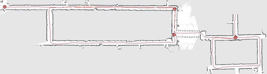
6

Algorithm 1 Improved RBPF for Map Learning                             the Gaussian approximation of the odometry motion model
Require:                                                               described in [41]. We obtain this approximation through Taylor
  St−1 , the sample set of the previous time step                      expansion in an EKF-style procedure. In general, there are
  zt , the most recent laser scan                                      more sophisticated techniques estimating the motion of the
  ut−1 , the most recent odometry measurement                          robot. However, we use that model to estimate a movement
Ensure:                                                                between two filter updates which is performed after the robot
  St , the new sample set                                              traveled around 0.5 m. In this case, this approximation works
                                                                       well and we did not observed a significant difference between
  St = {}                                                              the EKF-like model and the in general more accurate sample-
            (i)
  for all st−1 ∈ St−1 do                                               based velocity motion model [41].
         (i)    (i)  (i)     (i)
    < xt−1 , wt−1 , mt−1 >= st−1
                                                                                              V. C OMPLEXITY
    // scan-matching                                                       This section discusses the complexity of the presented
      ′(i)   (i)                                                       approach to learn grid maps with a Rao-Blackwellized particle
    xt = xt−1 ⊕ ut−1
      (i)                (i)         ′(i)
    x̂t = argmaxx p(x | mt−1 , zt , xt )                               filter. Since our approach uses a sample set to represent the
                                                                       posterior about maps and poses, the number N of samples
        (i)
    if x̂t = failure then                                              is the central quantity. To compute the proposal distribution,
         (i)             (i)                                           our approach samples around the most likely position reported
       xt ∼ p(xt | xt−1 , ut−1 )
          (i)    (i)           (i)   (i)                               by the scan-matcher. This sampling is done for each particle
       wt = wt−1 · p(zt | mt−1 , xt )                                  a constant number of times (K) and there is no dependency
    else                                                               between the particles when computing the proposal. Further-
       // sample around the mode                                       more, the most recent observation zt used to compute µ(i)
       for k = 1, . . . , K do                                         and Σ(i) covers only an area of the map m (bounded by the
           xk ∼ {xj | |xj − x̂(i) | < ∆}                               odometry error and the maximum range of the sensor), so the
       end for                                                         complexity depends only on the number N of particles. The
                                                                       same holds for the update of the individual maps associated
       // compute Gaussian proposal                                    to each of the particles.
         (i)
       µt = (0, 0, 0)T                                                     During the resampling step, the information associated to a
       η (i) = 0                                                       particle needs to be copied. In the worst case, N − 1 samples
       for all xj ∈ {x1 , . . . , xK } do                              are replaced by a single particle. In our current system, each
             (i)      (i)               (i)                 (i)
           µt = µt +xj ·p(zt | mt−1 , xj )·p(xt | xt−1 , ut−1 )        particle stores and maintains its own grid map. To duplicate
                                    (i)                 (i)
           η (i) = η (i) + p(zt | mt−1 , xj ) · p(xt | xt−1 , ut−1 )   a particle, we therefore have to copy the whole map. As a
       end for                                                         result, a resampling action introduces a worst case complexity
         (i)      (i)
       µt = µt /η (i)                                                  of O(N M ), where M is the size of the corresponding grid
          (i)
       Σt = 0                                                          map. However, using the adaptive resampling technique, only
       for all xj ∈ {x1 , . . . , xK } do                              very few resampling steps are required during mapping.
              (i)      (i)                                                 To decide whether or not a resampling is needed, the
           Σt = Σt + (xj − µ(i) )(xj − µ(i) )T ·
                             (i)                 (i)
                   p(zt | mt−1 , xj ) · p(xj | xt−1 , ut−1 )           effective sample size (see Eq. (20)) needs to be taken into
       end for                                                         account. Again, the computation of the quantity introduces a
          (i)      (i)
       Σt = Σt /η (i)                                                  complexity of O(N ).
       // sample new pose                                                  As a result, if no resampling operation is required, the
         (i)           (i)
       xt ∼ N (µt , Σt )
                            (i)                                        overall complexity for integrating a single observation depends
                                                                       only linearly on the number of particles. If a resampling is
       // update importance weights                                    required, the additional factor M which represents the size of
          (i)   (i)
       wt = wt−1 · η (i)                                               the map is introduced and leads to a complexity of O(N M ).
    end if                                                             The complexity of each individual operation is depicted in
    // update map                                                      Table I.
       (i)                   (i)   (i)                                     Note that the complexity of the resampling step can be
    mt = integrateScan(mt−1 , xt , zt )
                                                                       reduced by using a more intelligent map representation as
    // update sample set
                    (i)  (i)   (i)                                     done in DP-SLAM [9]. It can be shown, that in this case the
    St = St ∪ {< xt , wt , mt >}
                                                                       complexity of a resampling step is reduced to O(AN 2 log N ),
  end for
                                                                       where A is the area covered by the sensor. However, building
                    1                                                  an improved map representation is not the aim of this paper.
  Neff = PN                    2
              i=1
                    (w̃(i) )                                           We actually see our approach as orthogonal to DP-SLAM
                                                                       because both techniques can be combined. Furthermore, in
  if Neff < T then
                                                                       our experiments using real world data sets, we figured out
     St = resample(St )
                                                                       the resampling steps are not the dominant part and they occur
  end if
                                                                       rarely due to the adaptive resampling strategy.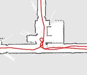
7
TABLE I
C OMPLEXITY OF THE DIFFERENT OPERATIONS FOR INTEGRATING ONE
OBSERVATION .
Operation Complexity
Computation of the proposal distribution O(N )
Update of the grid map O(N )
Computation of the weights O(N )
Test if resampling is required O(N )
Resampling O(N M )
Fig. 5. The Freiburg Campus. The robot first runs around the external
perimeter in order to close the outer loop. Afterwards, the internal parts of
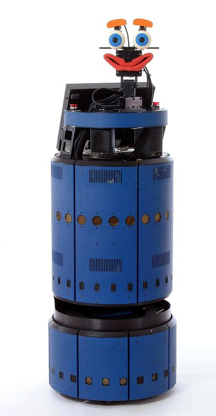
Fig. 3. Different types of robot used to acquire real robot data used for the campus are visited. The overall trajectory has a length of 1.75 km and
mapping (ActivMedia Pioneer 2 AT, Pioneer 2 DX-8, and an iRobot B21r). covers an area of approximately 250 m by 250 m. The depicted map was
generated using 30 particles.
VI. E XPERIMENTS
A. Mapping Results
The approach described above has been implemented and
tested using real robots and datasets gathered with real robots. The datasets discussed here have been recorded at the Intel
Our mapping approach runs online on several platforms like Research Lab in Seattle, at the campus of the University of
ActivMedia Pioneer2 AT, Pioneer 2 DX-8, and iRobot B21r Freiburg, and at the Killian Court at MIT. The maps of these
robots equipped with a SICK LMS and PLS laser range environments are depicted in Figures 4, 5, and 6.
finders (see Figure 3). The experiments have been carried a) Intel Research Lab: The Intel Research Lab is de-
out in a variety of environments and showed the effective- picted in the left image of Figure 4 and has a size of 28 m
ness of our approach in indoor and outdoor settings. Most by 28 m. The dataset has been recorded with a Pioneer II
of the maps generated by our approach can be magnified robot equipped with a SICK sensor. To successfully correct
up to a resolution of 1 cm, without observing considerable this dataset, our algorithm needed only 15 particles. As can
inconsistencies. Even in big real world datasets covering an be seen in the right image of Figure 4, the quality of the final
area of approximately 250 m by 250 m, our approach never map is so high that the map can be magnified up to 1 cm of
required more than 80 particles to build accurate maps. In resolution without showing any significant errors.
the reminder of this section, we discuss the behavior of the b) Freiburg Campus: The second dataset has been
filter in different datasets. Furthermore, we give a quantitative recorded outdoors at the Freiburg campus. Our system needed
analysis of the performance of the presented approach. Highly only 30 particles to produce a good quality map such as the
accurate grid maps have been generated with our approach one shown in Figure 5. Note that this environment partly
from several datasets. These maps, raw data files, and an violates the assumptions that the environment is planar. Ad-
efficient implementation of our mapping system are available ditionally, there were objects like bushes and grass as well
on the web [38]. as moving objects like cars and people. Despite the resulting
spurious measurements, our algorithm was able to generate an
accurate map.
c) MIT Killian Court: The third experiment was per-
formed with a dataset acquired at the MIT Killian court1
and the resulting map is depicted in Figure 6. This dataset is
extremely challenging since it contains several nested loops,
which can cause a Rao-Blackwellized particle filter to fail due
to particle depletion. Using this dataset, the selective resam-
pling procedure turned out to be important. A consistent and
topologically correct map can be generated with 60 particles.
However, the resulting maps sometimes show artificial double
walls. By employing 80 particles it is possible to achieve high
Fig. 4. The Intel Research Lab. The robot starts in the upper part of the
quality maps.
circular corridor, and runs several times around the loop, before entering the
rooms. The left image depicts the resulting map generated with 15 particles. 1 Note that there exist two different versions of that dataset on the web.
The right image shows a cut-out with 1 cm grid resolution to illustrate the One has a pre-corrected odometry and the other one has not. We used the
accuracy of the map in the loop closure point. raw version without pre-corrected odometry information.8
g f
100
Neff/N [%]
75
50
a 25
A B C D
time
e
Fig. 8. The graph plots the evolution of the Neff function over time during
an experiment in the environment shown in the top image. At time B the
robot closes the small loop. At time C and D resampling actions are carried
d c after the robots closes the big loop.
b
algorithm in the environments considered here. The plots show
the percentage of correctly generated maps, depending on the
number of particles used. The question if a map is consistent or
Fig. 6. The MIT Killian Court. The robot starts from the point labeled a not has been evaluated by visual inspection in a blind fashion
and then traverses the first loop labeled b. It then moves through the loops (the inspectors were not the authors). As a measure of success,
labeled c, d and moves back to the place labeled a and the loop labeled b. It
the visits the two big loops labeled f and g. The environment has a size of
we used the topological correctness.
250 m by 215 m and the robot traveled 1.9 km. The depicted map has been
generated with 80 particles. The rectangles show magnifications of several
parts of the map. C. Effects of Improved Proposals and Adaptive Resampling
The increased performance of our approach is due to
TABLE II
the interplay of two factors, namely the improved proposal
T HE NUMBER OF PARTICLES NEEDED BY OUR ALGORITHM COMPARED TO
distribution, which allows us to generate samples with an
THE APPROACH OF H ÄHNEL et al. [16].
high likelihood, and the adaptive resampling controlled by
Proposal Distribution Intel MIT Freiburg
our approach 8 60 20
monitoring Neff . For proposals that do not consider the whole
approach of [16] 40 400 400 input history, it has been proven that Neff can only decrease
(stochastically) over time [7]. Only after a resampling opera-
tion, Neff recovers its maximum value. It is important to notice
B. Quantitative Results that the behavior of Neff depends on the proposal: the worse
the proposal, the faster Neff drops.
In order to measure the improvement in terms of the number
We found that the evolution of Neff using our proposal
of particles, we compared the performance of our system using
distribution shows three different behaviors depending on the
the informed proposal distribution to the approach done by
information obtained from the robot’s sensors. Figure 8 illus-
Hähnel et al. [16]. Table II summarizes the number of particles
trates the evolution of Neff during an experiment. Whenever
needed by a RBPF for providing a topologically correct map
the robot moves through unknown terrain, Neff typically drops
in at least 60% of all applications of our algorithm.
slowly. This is because the proposal distribution becomes
It turns out that in all of the cases, the number of particles
less peaked and the likelihoods of observations often differ
required by our approach was approximately one order of
slightly. The second behavior can be observed when the robot
magnitude smaller than the one required by the other approach.
moves through a known area. In this case, each particle keeps
Moreover, the resulting maps are better due to our improved
localized within its own map due to the improved proposal
sampling process that takes the last reading into account.
distribution and the weights are more or less equal. This
Figure 7 summarizes results about the success ratio of our
results in a more or less constant behavior of Neff . Finally,
when closing a loop, some particles are correctly aligned with
100 their map while others are not. The correct particles have a
success rate [%]
Intel Lab
80 Freiburg Campus high weight, while the wrong ones have a low weight. Thus
MIT
60 MIT-2 the variance of the importance weights increases and Neff
40
20
substantially drops.
0 Accordingly, the threshold criterion applied on Neff typi-
10 100 1000 cally forces a resampling action when the robot is closing a
number of particles loop. In all other cases, the resampling is avoided and in this
Fig. 7. Success rate of our algorithm in different environments depending
way the filter keeps a variety of samples in the particle set.
on the number of particles. Each success rate was determined using 20 runs. As a result, the risk of particle depletion problem is seriously
For the experiment MIT-2 we disabled the adaptive resampling. reduced. To analyze this, we performed an experiment in9
Fig. 10. The effect of considering the odometry in the computation of the
proposal on the particle cloud. The left image depicts the particle distribution
if only the laser range finder data is used. By taking into account the odometry
when computing the proposal distribution, the particles can be drawn in a more
accurate manner. As can be seen in the right image, the particle cloud is more
focused, because it additionally incorporates the odometry information.
D. The Influence of the Odometry on the Proposal
This experiment is designed to show the advantage of the
proposal distribution, which takes into account the odome-
try information to draw particles. In most cases, the purely
laser-based proposal like the one presented in our previous
approach [14] is well-suited to predict the motion of the
particles. However, in a few situations the knowledge about
the odometry information can be important to focus the
proposal distribution. This is the case if only very poor features
are available in the laser data that was used to compute
the parameters of the Gaussian proposal approximation. For
example, an open free space without any obstacles or a long
featureless corridor can lead to high variances in the computed
proposal that is only based on laser range finder data. Figure 10
illustrates this effect based on simulated laser data.
In a further experiment, we simulated a short-range laser
scanner (like, e.g., the Hokuyo URG scanner). Due to the
maximum range of 4 m, the robot was unable to see the
end of the corridor in most cases. This results in an high
pose uncertainty in the direction of the corridor. We recorded
several trajectories in this environment and used them to
learn maps with and without considering the odometry when
computing the proposal distribution. In this experiment, the
approach considering the odometry succeeded in 100% of all
cases to learn a topologically correct map. In contrast to that,
our previous approach which does not take into account the
odometry succeeded only in 50% of all cases. This experiment
indicates the importance of the improved proposal distribution.
Figure 11 depicts typical maps obtained with the different
Fig. 9. Maps from the ACES building at University of Texas, the 4th floor proposal distributions during this experiment. The left map
of the Sieg Hall at the University of Washington, the Belgioioso building, and
building 101 at the University of Freiburg.
contains alignment errors caused by the high pose uncertainty
in the direction of the corridor. In contrast to that, a robot that
also takes into account the odometry was able to maintain the
which we compared the success rate of our algorithm to that correct pose hypotheses. A typical example is depicted in the
of a particle filter which resamples at every step. As Figure 7 right image.
illustrates, our approach more often converged to the correct Note that by increasing the number of particles, both ap-
solution (MIT curve) for the MIT dataset compared to the proaches are able to map the environment correctly in 100%
particle filter with the same number of particles and a fixed of all cases, but since each particle carries its own map, it
resampling strategy (MIT-2 curve). is of utmost importance to keep the number of particles as
low as possible. Therefore, this improved proposal is a means
to limit the number of particles during mapping with Rao-
To give a more detailed impression about the accuracy of Blackwellized particle filters.
our new mapping technique, Figure 9 depicts maps learned
from well known and freely available [18] real robot datasets
recorded at the University of Texas, at the University of E. Situations in Which the Scan-Matcher Fails
Washington, at Belgioioso, and at the University of Freiburg. As reported in Section III, it can happen that the scan-
Each map was built using 30 particles to represent the posterior matcher is unable to find a good pose estimate based on
about maps and poses. the laser range data. In this case, we sample from the raw10
TABLE III
AVERAGE EXECUTION TIME USING A STANDARD PC.
Operation Average Execution Time
Computation of the proposal distribu- 1910 ms
alignment tion, the weights, and the map update
errors Test if resampling is required 41 ms
Resampling 244 ms
VII. R ELATED W ORK
Mapping techniques for mobile robots can be roughly clas-
sified according to the map representation and the underlying
Fig. 11. Different mapping results for the same data set obtained using
the proposal distribution which ignores the odometry (left image) and which estimation technique. One popular map representation is the
considers the odometry when drawing the next generation of particles (right occupancy grid [31]. Whereas such grid-based approaches
image). are computationally expensive and typically require a huge
amount of memory, they are able to represent arbitrary objects.
odometry model to obtain the next generation of particles. In Feature-based representations are attractive because of their
most tested indoor dataset, however, such a situation never compactness. However, they rely on predefined feature extrac-
occurred at all. In the MIT dataset, this effect was observed tors, which assumes that some structures in the environments
once due to a person walking directly in front of the robot are known in advance.
while the robot was moving though a corridor that mainly The estimation algorithms can be roughly classified ac-
consists of glass panes. cording to their underlying basic principle. The most pop-
In outdoor datasets, such a situation can occur if the robot ular approaches are extended Kalman filters (EKFs), maxi-
moves through large open spaces because in this case the laser mum likelihood techniques, sparse extended information filters
range finder mainly reports maximum range readings. While (SEIFs), smoothing techniques, and Rao-Blackwellized parti-
mapping the Freiburg campus, the scan-matcher also reported cle filters. The effectiveness of the EKF approaches comes
such an error at one point. In this particular situation, the robot from the fact that they estimate a fully correlated posterior
entered the parking area (in the upper part of the map, compare over landmark maps and robot poses [21, 37]. Their weakness
Figure 5). On that day, all cars were removed from the parking lies in the strong assumptions that have to be made on both
area due to construction work. As a result, no cars or other the robot motion model and the sensor noise. Moreover, the
objects caused reflections of the laser beams and most parts landmarks are assumed to be uniquely identifiable. There exist
of the scan consisted of maximum range readings. In such techniques [33] to deal with unknown data association in the
a situation, the odometry information provides the best pose SLAM context, however, if these assumptions are violated, the
estimate and this information is used by our mapping system filter is likely to diverge [12]. Similar observations have been
to predict the motion of the vehicle. reported by Julier et al. [20] as well as by Uhlmann [43]. The
unscented Kalman filter described in [20] is one way of better
dealing with the non-linearities in the motion model of the
vehicle.
F. Runtime Analysis A popular maximum likelihood algorithm computes the
most likely map given the history of sensor readings by
In this last experiment, we analyze the memory and com- constructing a network of relations that represents the spatial
putational resources needed by our mapping system. We used constraints between the poses of the robot [8, 13, 15, 24].
a standard PC with a 2.8 GHz processor. We recorded the Gutmann et al. [15] proposed an effective way for constructing
average memory usage and execution time using the default such a network and for detecting loop closures, while running
parameters that allows our algorithm to learn correct maps for an incremental maximum likelihood algorithm. When a loop
nearly all real world datasets provided to us. In this setting, closure is detected, a global optimization on the network of
30 particles are used to represent the posterior about maps and relation is performed. Recently, Hähnel et al. [17], proposed
poses and a new observation, consisting of a full laser range an approach which is able to track several map hypotheses
scan, is integrated whenever the robot moved more than 0.5 m using an association tree. However, the necessary expansions
or rotated more than 25◦ . The Intel Research Lab dataset (see of this tree can prevent the approach from being feasible for
Figure 4) contains odometry and laser range readings which real-time operation.
have been recorded over 45 min. Our implementation required Thrun et al. [42] proposed a method to correct the poses
150 MB of memory to store all the data using a maps with a of robots based on the inverse of the covariance matrix. The
size of approx. 40 m by 40 m and a grid resolution of 5 cm. advantage of the sparse extended information filters (SEIFs)
The overall time to correct the log file using our software was is that they make use of the approximative sparsity of the
less than 30 min. This means that the time to record a log file information matrix and in this way can perform predictions
is around 1.5 times longer than the time to correct the log file. and updates in constant time. Eustice et al. [10] presented a
Table III depicts the average execution time for the individual technique to make use of exactly sparse information matrices
operations. in a delayed-state framework. Paskin [34] presented a solution11
to the SLAM problem using thin junction trees. In this way, poor laser features for localization are available, our approach
he is able to reduce the complexity compared to the EKF performs better than our previous one.
approaches since thinned junction trees provide a linear-time The computation of the proposal distribution is done in
filtering operation. a similar way as in FastSLAM-2 presented by Montemerlo
Folkessen et al. [11] proposed an effective approach for et al. [26]. In contrast to FastSLAM-2, our approach does
dealing with symmetries and invariants that can be found in not rely on predefined landmarks and uses raw laser range
landmark based representation. This is achieved by represent- finder data to acquire accurate grid maps. Particle filters using
ing each feature in a low dimensional space (measurement proposal distributions that take into account the most recent
subspace) and in the metric space. The measurement subspace observation are also called look-ahead particle filters. Moralez-
captures an invariant of the landmark, while the metric space Menéndez et al. [30] proposed such a method to more reliably
represents the dense information about the feature. A mapping estimate the state of a dynamic system where accurate sensors
between the measurement subspace and the metric space are available.
is dynamically evaluated and refined as new observations The advantage of our approach is twofold. Firstly, our algo-
are acquired. Such a mapping can take into account spatial rithm draws the particles in a more effective way. Secondly, the
constraints between different features. This allows the authors highly accurate proposal distribution allows us to utilize the
to consider these relations for updating the map estimate. effective sample size as a robust indicator to decide whether
Very recently, Dellaert proposed a smoothing method called or not a resampling has to be carried out. This further reduces
square root smoothing and mapping [2]. It has several ad- the risk of particle depletion.
vantages compared to EKF since it better covers the non-
linearities and is faster to compute. In contrast to SEIFs, it VIII. C ONCLUSIONS
furthermore provides an exactly sparse factorization of the In this paper, we presented an improved approach to learn-
information matrix. ing grid maps with Rao-Blackwellized particle filters. Our
In a work by Murphy, Doucet, and colleagues [6, 32], Rao- approach computes a highly accurate proposal distribution
Blackwellized particle filters (RBPF) have been introduced based on the observation likelihood of the most recent sensor
as an effective means to solve the SLAM problem. Each information, the odometry, and a scan-matching process. This
particle in a RBPF represents a possible robot trajectory allows us to draw particles in a more accurate manner which
and a map. The framework has been subsequently extended seriously reduces the number of required samples. Addition-
by Montemerlo et al. [28, 29] for approaching the SLAM ally, we apply a selective resampling strategy based on the
problem with landmark maps. To learn accurate grid maps, effective sample size. This approach reduces the number of
RBPFs have been used by Eliazar and Parr [9] and Hähnel unnecessary resampling actions in the particle filter and thus
et al. [16]. Whereas the first work describes an efficient map substantially reduces the risk of particle depletion.
representation, the second presents an improved motion model Our approach has been implemented and evaluated on data
that reduces the number of required particles. Based on the acquired with different mobile robots equipped with laser
approach of Hähnel et al., Howard presented an approach to range scanners. Tests performed with our algorithm in different
learn grid maps with multiple robots [19]. The focus of this large-scale environments have demonstrated its robustness and
work lies in how to merge the information obtained by the the ability of generating high quality maps. In these experi-
individual robots and not in how to compute better proposal ments, the number of particles needed by our approach often
distributions. was one order of magnitude smaller compared to previous
Bosse et al. [1] describe a generic framework for SLAM in approaches.
large-scale environments. They use a graph structure of local
maps with relative coordinate frames and always represent the
ACKNOWLEDGMENT
uncertainty with respect to a local frame. In this way, they
are able to reduce the complexity of the overall problem. This work has partly been supported by the Marie Curie
In this context, Modayil et al. [25] presented a technique program under contract number HPMT-CT-2001-00251, by the
which combines metrical SLAM with topological SLAM. The German Research Foundation (DFG) under contract number
topology is utilized to solve the loop-closing problem, whereas SFB/TR-8 (A3), and by the EC under contract number FP6-
metric information is used to build up local structures. Similar 004250-CoSy, FP6-IST-027140-BACS, and FP6-2005-IST-5-
ideas have been realized by Lisien et al. [22], which introduce muFly. The authors would like to acknowledge Mike Bosse
a hierarchical map in the context of SLAM. and John Leonard for providing us the dataset of the MIT
The work described in this paper is an improvement of the Killian Court, Patrick Beeson for the ACES dataset, and Dirk
algorithm proposed by Hähnel et al. [16]. Instead of using Hähnel for the Intel Research Lab, the Belgioioso, and the
a fixed proposal distribution, our algorithm computes an im- Sieg-Hall dataset.
proved proposal distribution on a per-particle basis on the fly.
This allows us to directly use the information obtained from R EFERENCES
the sensors while evolving the particles. The work presented [1] M. Bosse, P.M. Newman, J.J. Leonard, and S. Teller. An ALTAS
here is also an extension of our previous approach [14], which framework for scalable mapping. In Proc. of the IEEE Int. Conf. on
Robotics & Automation (ICRA), pages 1899–1906, Taipei, Taiwan, 2003.
lacks the ability to incorporate the odometry information into [2] F. Dellaert. Square Root SAM. In Proc. of Robotics: Science and
the proposal. Especially, in critical situations in which only Systems (RSS), pages 177–184, Cambridge, MA, USA, 2005.12
[3] F. Dellaert, D. Fox, W. Burgard, and S. Thrun. Monte carlo localization Artificial Intelligence (IJCAI), pages 1151–1156, Acapulco, Mexico,
for mobile robots. In Proc. of the IEEE Int. Conf. on Robotics & 2003.
Automation (ICRA), Leuven, Belgium, 1998. [27] M. Montemerlo, N. Roy, S. Thrun, D. Hähnel, C. Stachniss, and
[4] G. Dissanayake, H. Durrant-Whyte, and T. Bailey. A computationally J. Glover. CARMEN – the carnegie mellon robot navigation toolkit.
efficient solution to the simultaneous localisation and map building http://carmen.sourceforge.net, 2002.
(SLAM) problem. In Proc. of the IEEE Int. Conf. on Robotics & [28] M. Montemerlo and S. Thrun. Simultaneous localization and mapping
Automation (ICRA), pages 1009–1014, San Francisco, CA, USA, 2000. with unknown data association using FastSLAM. In Proc. of the IEEE
[5] A. Doucet. On sequential simulation-based methods for bayesian filter- Int. Conf. on Robotics & Automation (ICRA), pages 1985–1991, Taipei,
ing. Technical report, Signal Processing Group, Dept. of Engeneering, Taiwan, 2003.
University of Cambridge, 1998. [29] M. Montemerlo, S. Thrun, D. Koller, and B. Wegbreit. FastSLAM: A
[6] A. Doucet, J.F.G. de Freitas, K. Murphy, and S. Russel. Rao-Black- factored solution to simultaneous localization and mapping. In Proc. of
wellized partcile filtering for dynamic bayesian networks. In Proc. of the National Conference on Artificial Intelligence (AAAI), pages 593–
the Conf. on Uncertainty in Artificial Intelligence (UAI), pages 176–183, 598, Edmonton, Canada, 2002.
Stanford, CA, USA, 2000. [30] R. Morales-Menéndez, N. de Freitas, and D. Poole. Real-time monitor-
[7] A. Doucet, N. de Freitas, and N. Gordan, editors. Sequential Monte- ing of complex industrial processes with particle filters. In Proc. of the
Carlo Methods in Practice. Springer Verlag, 2001. Conf. on Neural Information Processing Systems (NIPS), pages 1433–
[8] T. Duckett, S. Marsland, and J. Shapiro. Fast, on-line learning of globally 1440, Vancover, Canada, 2002.
consistent maps. Journal of Autonomous Robots, 12(3):287 – 300, 2002. [31] H.P. Moravec. Sensor fusion in certainty grids for mobile robots. AI
[9] A. Eliazar and R. Parr. DP-SLAM: Fast, robust simultainous local- Magazine, pages 61–74, Summer 1988.
ization and mapping without predetermined landmarks. In Proc. of the [32] K. Murphy. Bayesian map learning in dynamic environments. In
Int. Conf. on Artificial Intelligence (IJCAI), pages 1135–1142, Acapulco, Proc. of the Conf. on Neural Information Processing Systems (NIPS),
Mexico, 2003. pages 1015–1021, Denver, CO, USA, 1999.
[10] R. Eustice, H. Singh, and J.J. Leonard. Exactly sparse delayed-state [33] J. Neira and J.D. Tardós. Data association in stochastic mapping
filters. In Proc. of the IEEE Int. Conf. on Robotics & Automation (ICRA), using the joint compatibility test. IEEE Transactions on Robotics and
pages 2428–2435, Barcelona, Spain, 2005. Automation, 17(6):890–897, 2001.
[11] J. Folkesson, P. Jensfelt, and H. Christensen. Vision SLAM in the [34] M.A. Paskin. Thin junction tree filters for simultaneous localization and
measurement subspace. In Proc. of the IEEE Int. Conf. on Robotics mapping. In Proc. of the Int. Conf. on Artificial Intelligence (IJCAI),
& Automation (ICRA), pages 325–330, April 2005. pages 1157–1164, Acapulco, Mexico, 2003.
[12] U. Frese and G. Hirzinger. Simultaneous localization and mapping [35] M.K. Pitt and N. Shephard. Filtering via simulation: auxilary particle
- a discussion. In Proc. of the IJCAI Workshop on Reasoning with filters. Technical report, Department of Mathematics, Imperial College,
Uncertainty in Robotics, pages 17–26, Seattle, WA, USA, 2001. London, 1997.
[13] U. Frese, P. Larsson, and T. Duckett. A multilevel relaxation algorithm [36] N. Roy, M. Montemerlo, and S. Thrun. Perspectives on standardization
for simultaneous localisation and mapping. IEEE Transactions on in mobile robot programming. In Proc. of the IEEE/RSJ Int. Conf. on
Robotics, 21(2):1–12, 2005. Intelligent Robots and Systems (IROS), pages 2436–2441, Las Vegas,
[14] G. Grisetti, C. Stachniss, and W. Burgard. Improving grid-based NV, USA, 2003.
slam with Rao-Blackwellized particle filters by adaptive proposals and [37] R. Smith, M. Self, and P. Cheeseman. Estimating uncertain spatial
selective resampling. In Proc. of the IEEE Int. Conf. on Robotics & realtionships in robotics. In I. Cox and G. Wilfong, editors, Autonomous
Automation (ICRA), pages 2443–2448, Barcelona, Spain, 2005. Robot Vehicles, pages 167–193. Springer Verlag, 1990.
[15] J.-S. Gutmann and K. Konolige. Incremental mapping of large cyclic [38] C. Stachniss and G. Grisetti. Mapping results obtained with
environments. In Proc. of the IEEE Int. Symposium on Computational Rao-Blackwellized particle filters. http://www.informatik.uni-
Intelligence in Robotics and Automation (CIRA), pages 318–325, Mon- freiburg.de/∼stachnis/research/rbpfmapper/, 2004.
terey, CA, USA, 1999. [39] S. Thrun. An online mapping algorithm for teams of mobile robots.
[16] D. Hähnel, W. Burgard, D. Fox, and S. Thrun. An efficient FastSLAM Int. Journal of Robotics Research, 20(5):335–363, 2001.
algorithm for generating maps of large-scale cyclic environments from [40] S. Thrun, W. Burgard, and D. Fox. Probabilistic Robotics, chapter Robot
raw laser range measurements. In Proc. of the IEEE/RSJ Int. Conf. on Perception, pages 171–172. MIT Press, 2005.
Intelligent Robots and Systems (IROS), pages 206–211, Las Vegas, NV, [41] S. Thrun, W. Burgard, and D. Fox. Probabilistic Robotics, chapter Robot
USA, 2003. Motion, pages 121–123. MIT Press, 2005.
[17] D. Hähnel, W. Burgard, B. Wegbreit, and S. Thrun. Towards lazy data [42] S. Thrun, Y. Liu, D. Koller, A.Y. Ng, Z. Ghahramani, and H. Durrant-
association in slam. In Proc. of the Int. Symposium of Robotics Research Whyte. Simultaneous localization and mapping with sparse extended
(ISRR), pages 421–431, Siena, Italy, 2003. information filters. Int. Journal of Robotics Research, 23(7/8):693–716,
[18] A. Howard and N. Roy. The robotics data set repository (Radish), 2003. 2004.
http://radish.sourceforge.net/. [43] J. Uhlmann. Dynamic Map Building and Localization: New Theoretical
[19] Andrew Howard. Multi-robot simultaneous localization and mapping Foundations. PhD thesis, University of Oxford, 1995.
using particle filters. In Robotics: Science and Systems, pages 201–208, [44] R. van der Merwe, N. de Freitas, A. Doucet, and E. Wan. The unscented
Cambridge, MA, USA, 2005. particle filter. Technical Report CUED/F-INFENG/TR380, Cambridge
[20] S. Julier, J. Uhlmann, and H. Durrant-Whyte. A new approach for fil- University Engineering Department, August 2000.
tering nonlinear systems. In Proc. of the American Control Conference,
pages 1628–1632, Seattle, WA, USA, 1995.
[21] J.J. Leonard and H.F. Durrant-Whyte. Mobile robot localization by
tracking geometric beacons. IEEE Transactions on Robotics and
Automation, 7(4):376–382, 1991.
[22] B. Lisien, D. Silver D. Morales, G. Kantor, I.M. Rekleitis, and H. Choset.
Hierarchical simultaneous localization and mapping. In Proc. of the
IEEE/RSJ Int. Conf. on Intelligent Robots and Systems (IROS), pages
448–453, Las Vegas, NV, USA, 2003.
[23] J.S. Liu. Metropolized independent sampling with comparisons to
rejection sampling and importance sampling. Statist. Comput., 6:113–
119, 1996.
[24] F. Lu and E. Milios. Globally consistent range scan alignment for
environment mapping. Journal of Autonomous Robots, 4:333–349, 1997.
[25] J. Modayil, P. Beeson, and B. Kuipers. Using the topological skeleton
for scalable global metrical map-building. In Proc. of the IEEE/RSJ
Int. Conf. on Intelligent Robots and Systems (IROS), pages 1530–1536,
Sendai, Japan, 2004.
[26] M. Montemerlo, S. Thrun D. Koller, and B. Wegbreit. FastSLAM 2.0:
An improved particle filtering algorithm for simultaneous localization
and mapping that provably converges. In Proc. of the Int. Conf. onYou can also read