A Bayesian method for point source polarisation estimation
←
→
Page content transcription
If your browser does not render page correctly, please read the page content below
A&A 651, A24 (2021)
https://doi.org/10.1051/0004-6361/202039741                                                                        Astronomy
c ESO 2021                                                                                                          &
                                                                                                                   Astrophysics

          A Bayesian method for point source polarisation estimation
                  D. Herranz1 , F. Argüeso2,4 , L. Toffolatti3,4 , A. Manjón-García1,5 , and M. López-Caniego6

      1
          Instituto de Física de Cantabria, CSIC-UC, Av. de Los Castros s/n, 39005 Santander, Spain
          e-mail: herranz@ifca.unican.es
      2
          Departamento de Matemáticas, Universidad de Oviedo, C. Federico García Lorca 18, 33007 Oviedo, Spain
      3
          Departamento de Física, Universidad de Oviedo, C. Federico García Lorca 18, 33007 Oviedo, Spain
      4
          Instituto Universitario de Ciencias y Tecnologías Espaciales de Asturias (ICTEA), Escuela de Ingeniería de Minas, Materiales y
          Energía de Oviedo, C. Independencia 13, 33004 Oviedo, Spain
      5
          Departamento de Física Moderna, Universidad de Cantabria, 39005 Santander, Spain
      6
          ESAC, Camino Bajo del Castillo s/n, 28692 Villafranca del Castillo, Madrid, Spain

      Received 22 October 2020 / Accepted 2 March 2021

                                                                  ABSTRACT

      The estimation of the polarisation P of extragalactic compact sources in cosmic microwave background (CMB) images is a very
      important task in order to clean these images for cosmological purposes –for example, to constrain the tensor-to-scalar ratio of
      primordial fluctuations during inflation– and also to obtain relevant astrophysical information about the compact sources themselves
      in a frequency range, ν ∼ 10–200 GHz, where observations have only very recently started to become available. In this paper, we
      propose a Bayesian maximum a posteriori approach estimation scheme which incorporates prior information about the distribution
      of the polarisation fraction of extragalactic compact sources between 1 and 100 GHz. We apply this Bayesian scheme to white noise
      simulations and to more realistic simulations that include CMB intensity, Galactic foregrounds, and instrumental noise with the
      characteristics of the QUIJOTE (Q U I JOint TEnerife) experiment wide survey at 11 GHz. Using these simulations, we also compare
      our Bayesian method with the frequentist filtered fusion method that has been already used in the Wilkinson Microwave Anisotropy
      Probe data and in the Planck mission. We find that the Bayesian method allows us to decrease the threshold for a feasible estimation
      of P to levels below ∼100 mJy (as compared to ∼500 mJy which was the equivalent threshold for the frequentist filtered fusion). We
      compare the bias introduced by the Bayesian method and find it to be small in absolute terms. Finally, we test the robustness of the
      Bayesian estimator against uncertainties in the prior and in the flux density of the sources. We find that the Bayesian estimator is
      robust against moderate changes in the parameters of the prior and almost insensitive to realistic errors in the estimated photometry
      of the sources.
      Key words. methods: data analysis – techniques: image processing – polarization – cosmic background radiation –
      radio continuum: galaxies

1. Introduction                                                           (2019) could extend the analysis of polarisation properties of
                                                                          ERS performed by Galluzzi et al. (2018) up to 97.5 GHz, by
The polarisation properties of extragalactic radio sources (ERS)          polarimetric observations of a complete sample of 32 extragalac-
–that is to say radio galaxies, radio loud quasars, blazars, etc.–        tic radio sources. Their findings show that the distribution of the
are not well constrained even at centimetre wavelengths, given            observed Π fractions is, again, well fitted by a log-normal distri-
that the total linear polarisation of ERS, P, in general consti-          bution, thus confirming previous outcomes at lower frequencies
tutes a small fraction of their total flux density, S . The observed      (Massardi et al. 2013; Galluzzi et al. 2018) and also the predic-
value of P being typically a few per cent, with only very few             tions of Tucci & Toffolatti (2012). The analysis of Galluzzi et al.
ERS showing a total polarisation fraction, Π = P/S , as high as           (2019) also confirms the absence of any statistically significant
∼10 per cent of the total flux density (e.g., Sajina et al. 2011;         trend of polarisation properties of ERS with the frequency or the
Tucci & Toffolatti 2012). Moreover, at shorter wavelengths, that          flux density.
is at λ ≤ 1 cm, these properties are still poorly known due to                 Recent analyses of the ERS present in the full sky cosmic
the difficulty of properly calibrating in the radio to millimetre         microwave background (CMB) anisotropy maps in polarisation
regime that afflicted the polarisation experiments until a few            provided by the European Space Agency (ESA) Planck mis-
years ago. However, the knowledge of the total and polarisa-              sion (Planck Collaboration I 2016; Planck Collaboration XXVI
tion fraction of ERS is rapidly improving at high radio frequen-          2016) also indicate typical median polarisation fractions of ERS
cies thanks to large samples of sources mainly observed by the            of 2−3% at frequencies as high as 300 GHz (Bonavera et al.
Australia Telescope Compact Array (ATCA) and by the Very                  2017a,b; Trombetti et al. 2018). Therefore, an accurate charac-
Large Array (VLA; Sadler et al. 2006; López-Caniego et al.                terisation of polarisation properties of ERS as well as their effi-
2009; Massardi et al. 2008, 2011, 2013; Murphy et al. 2010;               cient detection and subtraction from CMB maps is especially
Jackson et al. 2010; Galluzzi et al. 2017, 2018). More recently,          crucial for measuring the primordial CMB B-mode polarisa-
and thanks to the very high sensitivity of the new detectors of           tion down to values of the tensor to scalar ratios r ∼ 0.001,
the Atacama Large Millimetre Array (ALMA), Galluzzi et al.                which could be achievable by future space probes (i.e. LiteBird:

                                                      Article published by EDP Sciences                                        A24, page 1 of 13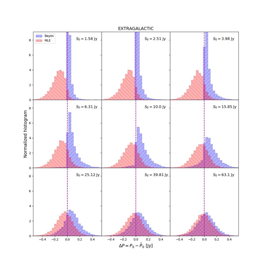
A&A 651, A24 (2021)

Sekimoto et al. 2018; COrE: Delabrouille et al. 2018). We                     parameters) can be treated separately as independent images to
remind readers that the simulations by Remazeilles et al. (2018)              which any of the standard compact component separation tech-
have shown that at these low values of r, unresolved polarised                niques could be applied. The main difference with respect to the
ERS can probably be the dominant foreground at multipoles                     classical setting is that, unlike the total flux density S , which is
` > 50 in the power spectrum of the CMB anisotropy. These                     always non-negative, Q and U can be either positive, negative,
results have been confirmed by Puglisi et al. (2018) by exploit-              or zero. From a physical point of view, however, it makes more
ing the state-of-the-art data sets on polarised point sources over            sense to process the polarisation data jointly (see Herranz et al.
the 1.4–217 GHz frequency range.                                              2012, for a review on the   p topic). In particular, the total polari-
    In addition to the essential information that the polarisation            sation of a source P = Q2 + U 2 and its polarisation fraction
of ERS provides about the structure and evolution of extragalac-              Π = P/S are directly related to the physical processes occurring
tic baryonic matter at low to intermediate redshifts, the study               along the path of photons from the ERS to Earth, while Q and U
of this polarised radiation is paramount for cosmology, and in                are frame-dependent quantities lacking in physical meaning on
particular for CMB science. ERS detection and subtraction is                  themselves.
a fundamental part of the component separation process neces-                      The two main problems arising when dealing with P are the
sary to achieve the science goals set for the next generation of              typically low signal-to-noise ratio of the polarisation signal com-
CMB experiments. In particular, ERS would significantly affect                ing from ERS and the non-Gaussian distribution of its noise
the estimation of the CMB polarisation angular power spectra                  statistics. Regarding the former, as mentioned above, the typi-
and, therefore, limit the ability of CMB experiments to constrain             cal polarisation fractions of ERS at frequencies below ∼10 GHz
cosmological parameters such as the tensor-to-scalar ratio r of               are at most 10%. This means that only a few ERS are bright
primordial perturbations during inflation. ERS could become an                enough to be detected in polarisation with present-day technol-
important obstacle for the detection of the primordial gravita-               ogy. A standard procedure to avoid false detections in polari-
tional wave background (PGWB) for low values of r (Tucci et al.               sation is to detect sources in total intensity and then to try to
2005; Puglisi et al. 2018; Trombetti et al. 2018) due to both the             estimate their polarisation properties in a non-blind way3 . We
additional noise they constitute in themselves and the reduction              follow this approach in this paper. Regarding the latter prob-
in delensing power they cause by degrading lensing potential                  lem, assuming that the Q and U noises are Gaussian-distributed,
reconstructions (see, e.g., Sailer et al. 2020). Therefore, during            P would have a non-Gaussian Rice distribution (Rice 1945).
recent years, the interest in the development of signal processing            Rician distribution has strictly non-negative support and heavy
techniques specifically tailored for the detection and characteri-            tails, which firstly biases the estimation of the polarisation of
sation of ERS in CMB images has grown in the literature.                      the sources and secondly disrupts the intuitive interpretation of
    Signal processing techniques for the detection of polarised               signal-to-noise in terms of σ thresholds which is used virtually
ERS must take the spinorial nature of electromagnetic waves                   everywhere else in radio astronomy. Simmons & Stewart (1985)
into account. The signal can not only be described by one but as              discussed four estimators which attempted to correct for bias-
many as four independent components, one for the total inten-                 ing in the degree of linear polarisation in the presence of low
sity of the radiation field and three for its polarisation state. It is       signal-to-noise ratios. More recently, Argüeso et al. (2009) stud-
convenient to use the Stokes’ parameters S , Q, U, and V (S for               ied the problem in the context of CMB astronomy and developed
total intensity1 in terms of flux density, see, e.g., Galluzzi et al.         two methods for the detection and estimation of ERS in polari-
(2019), Q and U for linear polarisation, and V for circular polar-            sation data: one that applies the Neyman-Pearson lemma to the
isation), but other representations are also possible. The Stokes’            Rice distribution, the Neyman-Pearson filter (NPF), and another
V parameter is not usually considered since Thomson scatter-                  based on pre-filtering before fusion of Q and U to obtain P, the
ing does not induce circular polarisation in the CMB. Circular                filtered fusion (FF) method. That work found that under typi-
polarisation mechanisms in active galaxies have been described                cal CMB-experiment settings, the FF outperforms the NPF both
in the literature (see for example Rayner et al. 2000), but they              in terms of computational simplicity and accuracy, especially
are nonetheless considered to be sub-dominant in comparison to                for low fluxes. López-Caniego et al. (2009) applied the FF to
linear polarisation mechanisms. Therefore, in this paper we con-              the Wilkinson Microwave Anisotropy Probe (WMAP) five-year
sider, as it is customary2 , V = 0. Then the signal processing of             data. The same method has been used to study the polarisation
polarised ERS must deal with three independent quantities, two                of the Planck Second Catalogue of Compact Sources (PCCS2,
of them having the mathematical structure of a spinor field.                  Planck Collaboration XXVI 2016) and of the QUIJOTE experi-
    The S , Q, and U signals (or, alternatively, S , E, and B,                ment wide survey source catalogue (Herranz et al. 2021). Alter-
or any other set of three quantities obtained from the Stokes’                natively, a novel method for the estimation of the polarisation
                                                                              intensity and angle of compact sources in the E and B modes of
1
    The usual notation for this Stokes parameter is I. However, in this       polarisation based on steerable wavelets has been recently pro-
work we have changed the notation in order to avoid confusion between         posed by Diego-Palazuelos et al. (2021).
the intrinsic intensity of a source, which we refer to as S 0 later in this        All the previously mentioned methods attempt to estimate
paper, and the modified Bessel function of zero order, I0 , that appears      the ERS polarisation by minimising, as much as possible, the
in several equations in Sect. 2.                                              impact of noise and Galactic and extragalactic foregrounds on
2
    Foregrounds can produce circular polarisation under some circum-          the observed signal. The expected value of the polarisation does
stances, and it has been observed in a few extragalactic sources. The         not intervene in the estimation process. In other words, no a pri-
value of V is typically much lower than the other Stokes’ parameters. As      ori information is used in the estimation. Until very recently, this
it is explained in Sect. 2, the existence of sources with non-zero circu-
lar polarisation would not affect our estimations of the Q and U Stokes
                                                                              had been the most sensible choice as the polarisation properties
parameters. Of course, if there was a significant V term, neglecting it       of extragalactic sources were virtually unknown at microwave
would lead us to miss a part of the polarisation P. However, our method
                                                                              3
can be easily adapted to work with a third component in the form                 That is, focusing efforts on the precise position of the source once it
of an additional image –corresponding to the V Stokes’ parameter– if          has been detected in intensity, i.e. the non-blindness is only related to
necessary.                                                                    the positions of targets, not to any other quantity.

A24, page 2 of 13
D. Herranz et al.: A Bayesian method for point source polarisation estimation
frequencies. However, as recent experiments and facilities such (Crow & Shimizu 1988). Since P0 = ΠS 0 , if we assume that
as the ALMA, Planck, and the upgraded versions of ATCA and the value of S 0 is known, then the distribution of P0 is readily
VLA start shedding light on the λ ≤ 1 cm polarised sky, the pos- calculated
sibility of adding physical priors to our signal processing tech- 1 h i
g (P0 ) = √ exp − log P0 − µ1 2 /2σ2Π
niques is gradually opening. In this paper, we propose a Bayesian (3)
maximum a posteriori (MAP) method for the estimation of the 2πσΠ P0
polarisation properties of point sources. with µ1 = µ + log (S 0 ) = log (S 0 Πmed ). This assumption is
The structure of this paper is as follows. In Sect. 2 we review safe, since estimating S 0 is much simpler than estimating P0
the current observational evidence to construct physical priors and point sources for which the polarised emission is detectable
on the polarisation fraction of ERS and incorporate that infor- tend to have high flux densities. Therefore, we work, in general,
mation into two possible MAP estimators of the polarisation of with non-blind detection in polarisation. The knowledge of S 0
a compact source of known flux density S . These MAP esti- allowed us to write the joint probability distribution of P and P0 ,
mators take a form analogous to the Neyman-Pearson filter and h(P, P0 ) = f (P|P0 )g(P0 ), and by using Bayesâ theorem
FF by Argüeso et al. (2009), respectively, plus additional terms
that contain the a priori physical information on the probability h (P, P0 )
f (P0 |P) = (4)
distribution function of P for ERS. We call these two methods g(P)
Bayesian Rice and Bayesian filtered fusion (BFF), respectively.
with g(P) = h (P, P0 ) dP0 . Finally, by substituting Eqs. (1)
R
The BFF is easily applicable for both white and colour noise. For
this reason, and because in Argüeso et al. (2009) it was shown and (3) in Eq. (4), we obtain
that the FF outperforms the NPF, we focus on the BFF in the rest
(log P0 −µ1 )2 1
e−P0 /2σ I0 PP
2 2
h i
0
of the paper. In Sect. 3 we describe the simulations we used to σ2 exp − 2σΠ2 P0
test the BFF method. We first made simplistic simulations con- f (P0 |P) = R 2
. (5)
(log P0 −µ1 ) dP0
e−P0 /2σ I0 PP
2 2
h i
taining just white noise in Q and U and then we upgraded to real- σ2
0
exp − 2σ2 P0
Π
istic simulations with polarised Galactic foregrounds and CMB
emissions. In both cases, we used angular resolution, pixel scale, The integral in the denominator is just a normalisation. We have
and noise levels similar to the upcoming QUIJOTE experiment found the distribution of P0 given P, the posterior distribution,
wide survey data at 11 GHz (Rubino et al. 2021). The results of simply by assuming Gaussian noise in Q and U with the same
applying the BFF to our simulations are discussed in Sect. 4, dispersion and a log-normal pdf for Π (prior distribution). Every-
where we also provide a brief discussion about the robustness of thing has been calculated for a source located at a central pixel
the method against uncertainties on the priors and the determi- and without taking into account any information about the beam
nation of the total flux density of the sources. Finally, we draw and the data in a certain patch around the source. If we consider
our conclusions in Sect. 5. a polarised source at the central pixel of an n-pixel patch, a beam
with a spatial profile τ(x), and values of Pi for the polarisation
measured at each pixel i = 1, . . . , n, we can write the following
2. Method expression for the conditional pdf of P0 given the Pi values at
When we try to detect or estimate the polarisation P0 of a com- the different pixels:
pact source embedded in Gaussian noise, which can be a good
log P0 − µ1 2 1
approximation when dealing with sources present in CMB
p maps, f (P0 |Pi ) ∝ exp −
and when we consider the measured polarisation P = Q2 + U 2 2σ2Π P0
with similar Gaussian noise dispersions in Q and U, that is 2 τi Pi τi
2
Y
σQ = σU = σ, the distribution of P given P0 follows the Rice × exp −P0 2 I0 P0 2 . (6)
2σi σi
distribution i
Here Πi is the product symbol, τi is the profile at each pixel,
h i
f (P|P0 ) = P/σ2 exp − P2 + P20 /2σ2 I0 PP0 /σ2 . (1)
and σi is the noise dispersion (it could be different from pixel
This is the conditional probability distribution of P, the mea- to pixel). We took the natural logarithm from the right-hand side
sured polarisation, the given P0 , and the source polarisation, and changed sign, this is minus the log-posterior of the distribu-
with I0 being the modified Bessel function of zero order (Rice tion, save constant terms. In this way, we obtained a simplified
1945). This distribution has been used to obtain suitable esti- expression which we later minimised to find the estimator that
mators of P0 (Simmons & Stewart 1985; Argüeso et al. 2009; makes the posterior distribution maximum
López-Caniego et al. 2009; Herranz et al. 2012). However, no
log P0 − µ1 2
previous knowledge about P0 is assumed in these papers and − log f (P0 |Pi ) = + log (P0 ) + P20 z
this information, if available, could be very useful after being 2σ2Π
incorporated in a Bayesian scheme. Recently, relevant data about X
log I0 P0 yi + K
the distribution of the polarisation fraction at different fre- − (7)
quencies, Π = P0 /S 0 , with S 0 being the source flux density, i
have been presented (Massardi et al. 2013; Galluzzi et al. 2017, with
2019). According to these authors, this distribution can be rep- X τ2
resented by a log-normal probability density function (pdf) z= i
(8)
i
2σ2i
1 h i
g(Π) = √ exp −(log(Π) − µ)2 /2σ2Π , (2)
2πσΠ Π and
where µ = log Πmed –with Πmed being the median polarisa- Pi τi
yi = , (9)
tion fraction– and σΠ are easily obtained from hΠi and hΠ2 i σ2i
A24, page 3 of 13A&A 651, A24 (2021)
and where K is a constant term that encloses the proportionality adds the prior information, whereas the second term acts as a
terms not directly included in Eq. (7). If we differentiate with penalty for large values of the estimated polarisation, and finally
respect to P and equate to zero, the estimator P̂0 satisfies the last term is a constant that is irrelevant for the solution.
h i Now we can obtain the estimators Q̂0 and Û0 that minimise
log P̂0 − µ1 1 X I1 P̂0 yi the previous expression. Finally, we find
+ + 2P̂0 z − i yi = 0, (10)
P̂0 σ2Π
h
P̂0 i I0 P̂0 yi q
P̂0 = Q̂20 + Û02 (14)
with I1 being the modified Bessel function of order one. On the
other hand, in Argüeso et al. (2009), the FF method was shown
to perform better than the one derived from the Rice distribu- as our estimator of P0 . In all of these formulas, we have not con-
tion. The FF calculates the square root of the sum of the squares sidered the effect of the circular polarisation, V. As mentioned
of the maps in Q and U to which a matched filter has been previ- in the introduction, this effect is very small and can be neglected
ously applied. This method is just a maximisation of the condi- in general. At any rate, the generalisation of the Rice and FF
tional probability of the data Qi , Ui given the source polarisation methods to include circular polarisation has been presented in
Q0 , U0 , assuming that the noise is Gaussian with zero mean and Argüeso et al. (2011). However, in order to extend our Bayesian
independent for each pixel methods to this case, we would have to use a prior distribution
for V which is not known yet.
Y (Qi − Q0 τi )2 (Ui − U0 τi )2 To sum up the previous paragraphs: We have presented
f (Qi , Ui |Q0 , U0 ) = exp + . (11)
2σ2Qi 2σ2Ui four possible estimators of P0 , the old ones are the Rice
i
method and the FF (Argüeso et al. 2009; López-Caniego et al.
If we also assume that P0 follows a log-normal pdf and the 2009; Herranz et al. 2012; Planck Collaboration XXVI 2016),
polarisation angle distribution is uniform, we can combine the and the new ones, obtained by minimising the right-hand sides
previous formula with the prior distribution of Q0 , U0 and write, of Eqs. (7) and (12) or (13), which we call the Bayesian Rice
by applying Bayes’ theorem, minus the log-posterior of Q0 , U0 method and the Bayesian FF method, respectively. These new
given the data Qi , Ui methods incorporate, in a natural way, our information about the
q 2 source polarisation distribution. The FF and Rice methods are
log Q20 + U02 − µ1 implemented by minimising Eqs. (7) and (12)–(13) without the
− log f (Q0 , U0 |Qi , Ui ) = first two terms, which come from the Bayesian prior.
2σ2Π
+ log Q20 + U02
3. Simulations
X (Qi − Q0 τi )2
+ 3.1. White noise
i
2σ2Qi
X (Ui − U0 τi )2 As a first test bed to assess the performance of the Bayesian
+ + K. (12) techniques, we ran 10 000 simulations using only white noise as
i
2σ2Ui background for simulated sources. Table 1 shows the simulation
parameters for these simulations; the pixel size, beam full width
This expression could be very easily generalised, allowing even half maximum (FWHM), and white noise root mean square
the treatment of correlations between the noise in different pix- (rms) emulate those of the QUIJOTE (Rubiño-Martín et al.
els. In that case, Eq. (12) can be written as 2010, 2012; Génova-Santos et al. 2015; López-Caniego 2016)
q 2 experiment wide survey at 11 GHz (Rubino et al. 2021). We used
log Q20 + U02 − µ1 the same simulation parameters for the full sky simulations,
− log f (Q0 , U0 |Qi , Ui ) = which are discussed in Sect. 3.2.
2σ2Π For these white noise simulations, we directly created flat
images with uncorrelated Gaussian noise and at the centre we
+ log Q20 + U02
injected a point source with the FWHM listed in Table 1, a given
1X flux density S 0 , and polarisation fraction Π randomly drawn
+ (Qk − Q0 τk )t P−1Q,k (Qk − Q0 τk )
2 k from the log-normal distribution Eq. (2) with the mean and stan-
dard deviation values hΠi and σΠ described in Table 1. We sim-
1X
+ (Uk − U0 τk )t P−1
U,k (U k − U 0 τk )
ulated the intensities of S 0 in ten logarithmically spaced values
2 k between 0.1 and 100 Jy. In this way, we obtained a sample of
+ K, (13) sources from moderately faint to extra bright (and, since the
polarisation fraction follows distribution Eq. (2) with average
where the subindex k refers to the Fourier wave vector (or, for hΠi = 0.02, values of P from below 1 mJy to a few tens of
the case of spherical data, the appropriate spherical harmonic) Janskys).
and P x,k is the power spectrum (or angular power spectrum) of
the noise for the Stokes parameter x. This formula is expressed 3.2. Full sky simulations
in Fourier space for the sake of computational efficiency, but it
could also be expressed in real space by means of the correla- In order to assess the performance of our Bayesian techniques
tion matrix of the noise. In Eq. (13), it is clear that the third and under realistic conditions, we used realistic simulations of the
fourth terms on the right side of the equation are analogous to the QUIJOTE experiment wide survey (Rubino et al. 2021). The
matched filter on the Q and U maps, which in turn are the solu- QUIJOTE wide survey is observing approximately half the
tion of a maximum likelihood estimator (MLE). The first term sky at 11, 13, 17, and 19 GHz. These simulations have been
A24, page 4 of 13D. Herranz et al.: A Bayesian method for point source polarisation estimation
Table 1. Simulation parameters used for this work. rithmically spaced values between 0.1 and 100 Jy (that is, 200
sources–100 of them in the band, 100 of them outside it– with
Frequency (GHz) 11 S 0 = 0.1 Jy, 200 with S 0 = 0.2154 Jy, and so on). In this way,
FWHM (degrees) 0.85 we obtained a sample of sources from moderately faint to extra
Nside parameter 246 bright (and, since the polarisation fraction follows distribution
Pixel resolution (arcmin) 13.74 Eq. (2) with average hΠi = 0.02, values of P from below 1 mJy
White noise rms (Jy) 0.386 to a few tens of Janskys).
hΠi 0.02
σΠ 1.0 4. Results
4.1. White noise
produced thanks to the EU RADIOFOREGROUNDS project4 , In all the cases analysed with the white noise simulations, the
but they are not yet available publicly. The simulations make performance of the Bayesian FF at estimating the source polari-
use of the Planck Sky Model (PSM, Delabrouille et al. 2013), sation is better than that of the Bayesian Rice method. This was
a global representation of the multi-component sky at frequen- also the case for their non-Bayesian counterparts (Argüeso et al.
cies ranging from 1 GHz to 1 THz that summarises, in a syn- 2009, etc.). Due to this and in also taking into account that the
thetic way, as much of our present knowledge of the gigahertz generalisation of the Bayesian Rice method to full-sky simu-
sky as possible. The PSM is a public code5 developed mostly lations is far from trivial7 , from now on, we only compare the
by members of the Planck collaboration as a simulation tool Bayesian FF and the FF techniques.
for Planck activities and it makes it possible to simulate the The left panel of Fig. 4 shows the estimation of the polarised
sky in total intensity and the Q, U Stokes parameters for any flux density for the 10 000 white noise simulations. The results
experimental configuration in the gigahertz range. For this work, have been binned into eleven logarithmically spaced intervals in
we chose to simulate the QUIJOTE wide survey at 11 GHz. input P0 . In blue, we show the results from the Bayesian esti-
Figures 1 and 2 show the full Q Stokes wide survey simulated at mator Eq. (13). The error bars show the 68.27% intervals of the
11 GHz and the simulated QUIJOTE instrumental noise for the corresponding empirical distributions. The filled circles indicate
same Stokes parameter, area, and frequency. Table 1 indicates the median value of the distribution of results; the dots indi-
the main parameters used for this simulation. cate the average value of the distribution. For comparison, the
Formula (13) could be applied to the whole sky, but since results of a MLE, which correspond to the third and fourth terms
the statistical properties of the foregrounds vary strongly with of Eq. (13), are shown in orange. The red dotted line shows
Galactic latitude, we preferred to apply the Bayesian estimator the P = P0 line. The MLE is equivalent to the FF technique
locally. In order to test the method, we computed Eq. (13) on (Argüeso et al. 2009; López-Caniego et al. 2009; Herranz et al.
flat sky patches, projecting the HEALPix6 simulations described 2012). Both the Bayesian FF and the MLE estimator work well
above on 64 × 64 pixel (that is, a 14.658 × 14.658 square degrees for highly polarised sources (P0 & 0.5 Jy). For input polarisa-
area) planar images. tion levels below ∼0.2 Jy (which is approximately the rms of the
We ran the estimator on 2000 flat patches as described above. filtered noise of the simulations), however, the MLE reaches a
In order to study the effect of the level Galactic contamination, plateau: It is naturally limited by the level filtered noise. The
we divided the sky in two areas: 10 000 simulations within a Bayesian estimator, on the contrary, uses the a priori information
‘Galactic’ band with a Galactic latitude of |b| ≤ 10◦ and 10 000 on the Π distribution and the knowledge of the source flux den-
within an external region with |b| > 10◦ . The centre sky coor- sity S to predict lower P values. As a matter of fact, the Bayesian
dinate of each patch was chosen randomly, according to these FF tends to overcompensate and predict, for the lower end of val-
latitude intervals and inside the simulated wide survey observed ues of the input P0 , polarised fluxes Pest ∼ 0.2P0 . To see why this
area (see Figs. 1 and 2). For each patch, at the centre, we injected happens, we carried out a short theoretical calculation based on
a point source with the FWHM listed in Table 1, a given flux Eq. (12). The first part of Eq. (12) as a function of P0 is written
density S 0 , and polarisation fraction Π randomly drawn from below:
the log-normal distribution Eq. (2) with the mean and standard
deviation values hΠi and σΠ described in Table 1. It is important − log f (Q0 , U0 /Qi , Ui ) = (log P0 − log(Πmed S 0 ))2 /2σ2Π
to note that the PSM simulations already contain resolved and (Qi − Q0 τi )2
unresolved polarised point sources apart from the synthetic test + 2 log (P0 ) + Σi
2σ2i
sources we are injecting at the central position of each simulated
patch. Figure 3 shows the Q and U Stokes parameters for one (Ui − U0 τi )2
+ Σi + K. (15)
of our simulations. We simulated intensities of S 0 in ten loga- 2σ2i
4
The RADIOFOREGROUNDS project aims to combine two unique If we define
datasets, the nine Planck all-sky (30–857 GHz) maps and the four QUI-
Qi τi
JOTE Northern sky (10–20 GHz) maps, to provide the best possible Σi = P1 cos φ1 , Q0 = P0 cos φ (16)
characterisation of the physical properties of polarised emissions in the σ2i
microwave domain, together with an unprecedentedly thorough descrip-
tion of the intensity signal. This legacy information will be essential and
for future sub-orbital or satellite experiments. See more information in
Ui τi
http://www.radioforegrounds.eu/ Σi = P1 sin φ1 , U0 = P0 sin φ, (17)
5
http://www.apc.univ-paris7.fr/~delabrou/PSM/psm. σ2i
html
6 7
Hierarchical Equal Area isoLatitude Pixelation of a sphere, http: For spatially correlated noise, such as the polarisation produced by
//healpix.sf.net. Galactic foregrounds, the distribution of P is not Ricean anymore.
A24, page 5 of 13A&A 651, A24 (2021)
-13.9926 22.4137
Fig. 1. Q-Stokes simulated QUIJOTE wide survey sky at 11 GHz. The false colour bar is expressed in Janskys.
the previous formula can be expressed in terms of P0 , P1 and the Taking into account the values of hΠi and σΠ given in Table 1,
polarisation angles Πmed = 0.012 and we obtain
− log f (Q0 , U0 /Qi , Ui ) = (log P0 − log(Πmed S 0 ))2 /2σ2Π Pˆ0 = 0.00164 S 0 . (23)
+ 2 log (P0 ) − P0 P1 cos (φ − φ1 ) In order to check these theoretical results, we carried out 10 000
τ2i simulations with S 0 = 1 Jy. In this case, the noise, σ = 0.386 Jy,
+ P20 Σi + K2 (18) is much higher than the source polarisation. We find, for all
2σ2i our simulations, the estimated value hP̂0 i = 0.00166 ± 0.00002,
with which is compatible with the calculation above. Though the esti-
mator is constant in this case, this value is closer to the real value
Q2i + Ui2 than that obtained by using the matched filter, which is com-
Σi + K = K2 . (19) pletely dominated by the noise.
2σ2i
For higher values of S 0 , for example S 0 = 10 Jy, there
Taking the partial derivatives of Eq. (18) with respect to P0 and are around 5000 simulations, corresponding to the lower polar-
φ and equating them to zero, we obtain the estimators Pˆ0 and φ̂ isations, that produce an estimator close to the default value
that minimise minus the log-posterior. It can be easily seen that 0.016−0.020 Jy. For higher values of the real polarisation, there
φ̂ = φ1 and Pˆ0 is the solution of the following equation: is a combination of the prior and the matched filter terms in the
solution of (20). At any rate, the performance of the Bayesian FF
2 τ2i is better than that of the plain FF.
(log Pˆ0 − log(Πmed S 0 ))/σ2Π + 2 − Pˆ0 P1 + Pˆ0 Σi = 0. (20) The right panel of Fig. 4 shows the polarised flux estimation
σ2i
error8 as a function of the input flux density (temperature) of the
This equation is very interesting: If we assume that Pˆ0 P1
1 source S 0 . For low flux densities, the figure shows both the sys-
2 τ2 tematic overestimation of the MLE, due to the noise limit, and
and Pˆ0 Σi i2
1, that is, the source polarisation is much lower the underestimation of the Bayesian FF estimator due to the rea-
σi sons discussed above. In absolute terms, the statistical error of
than the noise, the estimation is dominated by the Bayesian prior the MLE is much larger than that of the Bayesian FF estimator
and in neglecting the last two terms in Eq. (20), we find a con- in the low flux density regime. There is an interesting interval
stant value for the estimator, independently of the data, at intermediate flux densities (∼10 Jy) at which the errors of the
2 MLE and Bayesian FF estimator are of the same order, but in
Pˆ0 = Πmed S 0 e−2σπ , (21) opposite directions. The Bayesian estimator seems to reach a
for a lognormal distribution and 8
Defined as P0 − P̂0 , where P0 is the input value and P̂0 is the esti-
mated value of the polarisation of the source either through the Bayesian
Πmed = hΠi exp −σ2Π /2 . (22) method or through the MLE.
A24, page 6 of 13D. Herranz et al.: A Bayesian method for point source polarisation estimation
-13.9934 7.84179
Fig. 2. Q-Stokes simulated QUIJOTE wide survey instrumental noise at 11 GHz. The false colour bar is expressed in Janskys. The non-uniformity
of the noise reflects the non-uniform sky scanning strategy of the telescope.
simulated Q map simulated U map
1.00
48 1.00 48
0.75 0.75
46 46
0.50 0.50
44 44
GLAT [deg]
GLAT [deg]
0.25 0.25
42 42
0.00 0.00
40 0.25 40
0.25
38 0.50 38
0.50
36 0.75 36 0.75
70 72 74 76 78 80 82 70 72 74 76 78 80 82
GLON [deg] GLON [deg]
(a) (b)
Fig. 3. Projected sky patches for one of our simulations. Map units are expressed in Janskys. (a) Stokes Q. (b) Stokes U.
plateau (i.e. is noise-limited) around P0 ∼ 10 mJy, a, order of 4.2. Full sky simulations
magnitude below in polarised flux than the MLE.
Figure 5 shows the absolute polarisation angle error, Figure 6 shows the estimation of the polarised flux density for
firstly the 10 000 ‘Galactic’ sky patches (|b| ≤ 10◦ ) and secondly
|∆φ| = |φ0 − φ̂0 |, (24)
the 10 000 ‘extragalactic’ (|b| > 10◦ ) simulated QUIJOTE sky
where φ0 and φ̂0 are the input and estimated polarisation angles patches. The results have been binned into eleven logarithmi-
(in degrees), as a function of the input polarisation of the source cally spaced intervals in input P0 . In blue, we show the results
P0 . The figure shows that there is little difference between the from the Bayesian estimator Eq. (13). The error bars show the
Galactic and extragalactic areas, and between the Bayesian esti- 68.27% intervals of the corresponding empirical distributions.
mator and the MLE. This is not a surprise, since the priors in For comparison, the results of a MLE, which correspond to the
Eq. (13) are constant with respect to φ0 , that is, the Bayesian third and fourths terms of Eq. (13), are shown in orange. The
estimator and the MLE should perform similarly, as is the case. MLE is equivalent to the FF technique (Argüeso et al. 2009;
A24, page 7 of 13A&A 651, A24 (2021)
sources at 11 GHz sources at 11 GHz
0.3
Bayesian Bayesian
Max. Likelihood Max. Likelihood
0.2
100
0.1
P0 P0 [Jy]
10 1 0.0
P0 [Jy]
0.1
10 2
0.2
0.3
10 2 10 1 100 100 101 102
P0 [Jy] S0 [Jy]
(a) (b)
Fig. 4. Left: binned estimates of the polarised flux density as a function of binned input P0 , in Janskys, for the set of 10 000 simulated white noise
patches. Right: error in the estimation P0 − P̂0 as a function of binned input S 0 (Jy) for the same set of simulations. Bayesian estimations appear in
blue, whereas maximum likelihood estimations are shown with an orange colour. Error bars show the 68.27% interval of the distribution of results
in each case. Filled circles indicate the median of the distribution; the diamonds (for the MLE) and crosses (for the Bayesian estimator) indicate
the average value of the distribution.
sources at 11 GHz Figure 7 shows the error of the estimation of P as a function
Bayesian of the input flux density of the sources (in Janskys). As in the
100 Max. Likelihood case of white noise, the MLE estimator tends to overestimate the
polarised flux of faint sources, whereas the Bayesian FF tends
to underestimate it. This error is a systematic bias that tends to
80
a constant value in relative terms, but decreases to zero Janskys
in absolute terms for S 0 → 0. Error bars are smaller for extra-
| | [deg]
60 galactic sources than for Galactic sources, which are embedded
in more intense foreground emission. Figures 8 and 9 show the
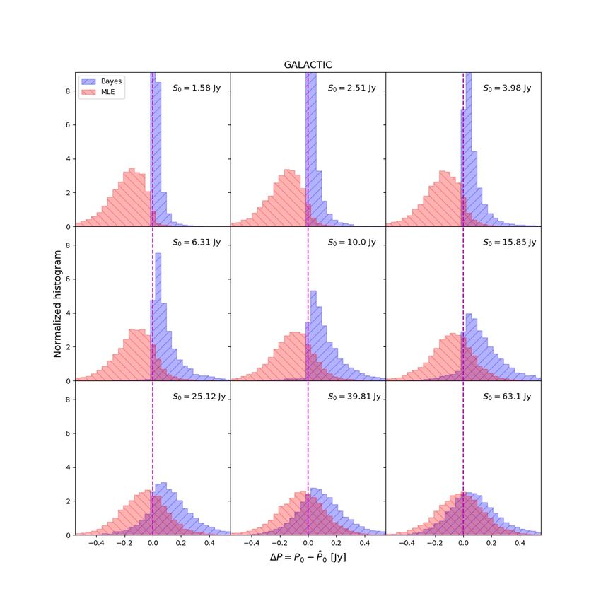
40 normalised histograms of the difference ∆P between the input
polarisation P0 and the estimated polarisation P,
20
∆P = P0 − P̂0 , (25)
0
10 2 10 1 100
P0 [Jy] for eleven different values of the total (Stokes I) flux density
S 0 . ‘Galactic’ sources are shown in Fig. 8 and ‘extragalactic’
Fig. 5. Binned estimates of |∆φ| = |φ0 − φ̂0 | as a function of binned sources are shown in Fig. 9. The estimation P̂0 has been obtained
input P0 , in Janskys, for the set of 10 000 simulated white noise images. with the BFF method introduced in this paper (in blue) and the
Bayesian estimations are marked with blue crosses and error bars,
whereas maximum likelihood estimations are shown with orange dia-
MLE (in red). For bright sources (S 0 > 10 Jy), the histograms
monds and error bars. The median values are indicated by means of are approximately symmetric and centred around ∆P = 0, but
large blue filled circles (Bayesian estimator) and small orange squares for fainter sources the MLE histograms are skewed to the left,
(MLE). showing the same kind of overestimation already observed in
Fig. 6. The histograms for the Bayesian estimator, however, are
skewed to the right but much narrower than the MLE histograms,
López-Caniego et al. 2009; Herranz et al. 2012). As it happened which indicates that the Bayesian estimator predicts the polari-
in the case of the white noise simulations (Sect. 4.1), for low sation of a source with a smaller margin of error. Both types
flux density sources the MLE estimator reaches a plateau domi- of error, MLE-overestimation and Bayesian FF-underestimation,
nated by the noise level (higher for Galactic than for extragalac- must be dealt with in CMB polarisation experiments, but the
tic sources). The Bayesian estimator reaches a similar plateau amount of bias is significantly smaller for the Bayesian FF
at much lower polarised fluxes, again in the ∼10 mJy regime estimator.
instead of the ∼100 mJy regime of the MLE. Please note, how- Finally, Fig. 10 shows the absolute polarisation angle error
ever, that the distribution of the estimated P̂0 by means of as a function of the input polarisation P0 . The figure shows that
the Bayesian estimator becomes more and more skewed as P0 there is little difference between the Galactic and extragalactic
decreases9 . areas and between the Bayesian estimator and the MLE. This
is not a surprise since the priors in Eq. (13) are constant with
9
This can be quickly seen by the growing differences between the respect to φ0 , that is, the Bayesian estimator and the MLE should
median and the average values of the distribution, as shown in the figure. perform similarly, as is the case.
A24, page 8 of 13D. Herranz et al.: A Bayesian method for point source polarisation estimation
Galactic sources at 11 GHz Extragalactic sources at 11 GHz
Bayesian Bayesian
Max. Likelihood Max. Likelihood
100 100
10 1 10 1
P0 [Jy]
P0 [Jy]
10 2 10 2
10 2 10 1 100 10 2 10 1 100
P0 [Jy] P0 [Jy]
(a) (b)
Fig. 6. Binned estimates of the polarised flux density as a function of binned input P0 , in Janskys, for the set of 10 000 simulated QUIJOTE sky
patches with |b| ≤ 10◦ (left) and the set of 10 000 simulated QUIJOTE sky patches with |b| > 10◦ (right) at 11 GHz. Bayesian estimations appear in
blue, whereas maximum likelihood estimations are shown with an orange colour. Error bars show the 68.27% interval of the distribution of results
in each case. Filled circles indicate the median of the distribution; the diamonds (for the MLE) and crosses (for the Bayesian estimator) indicate
the average value of the distribution.
Galactic sources at 11 GHz Extragalactic sources at 11 GHz
0.3 0.3
Bayesian Bayesian
Max. Likelihood Max. Likelihood
0.2 0.2
0.1 0.1
P0 P0 [Jy]
P0 P0 [Jy]
0.0 0.0
0.1 0.1
0.2 0.2
0.3 0.3
100 101 102 100 101 102
S0 [Jy] S0 [Jy]
(a) (b)
Fig. 7. Error in the estimation P0 − P̂0 (Jy) as a function of binned input S 0 (Jy) for the set of 10 000 simulated QUIJOTE sky patches with
|b| ≤ 10◦ (left) and the set of 10 000 simulated QUIJOTE sky patches with |b| > 10◦ (right) at 11 GHz. Bayesian estimations appear in blue,
whereas maximum likelihood estimations are shown with an orange colour. Error bars show the 68.27% interval of the distribution of results in
each case. Filled circles indicate the median of the distribution; the diamonds (for the MLE) and crosses (for the Bayesian estimator) indicate the
average value of the distribution.
4.3. A note on the robustness of the Bayesian estimator factor from 50% to 200%. Figure 11 shows the average estima-
tion error P0 − P̂0 as a function of the bias factor b. Error bars
Every time some prior information is used in the Bayesian show the 68.27% intervals of the corresponding empirical distri-
framework, one inevitably questions the effect a wrong guess butions. The figure shows that the average error of the Bayesian
has on the prior in the estimation. In order to shed some light estimator varies smoothly with the bias in the prior. For com-
on this, we re-analysed the one hundred simulations of ‘extra- parison, for the same simulations, the MLE produces a (bias
galactic’ sources with a flux density of S 0 = 10 Jy10 . Instead independent, as the maximum likelihood estimator does not use
of using the correct value of the median polarisation fraction prior information) value for the error P0 − P̂0 = −0.22 ± 0.12,
Πmed in Eq. (13), we used a biased parameter Πbmed = b Πmed which is larger than the Bayesian estimation (for this particu-
with b = [0.5, 0.6, . . . , 2.0], that is, we tested what happens if lar value of S 0 ) even when the prior is wrong by a factor of
our guess for the median polarisation fraction is wrong by a two.
10
We chose this particular flux density value because according to Another potential source of bias is the uncertainty on the true
Fig. 9 it marks the flux density for which the Bayesian estimator begins flux density of the source. The estimators in Eqs. (12) and (13)
to outperform the MLE. depend implicitly on an a priori knowledge of the source flux
A24, page 9 of 13A&A 651, A24 (2021)
Fig. 8. Normalised histogram of the difference ∆P between the input polarisation P0 and the estimated polarisation for the Bayesian estimator
(blue, /) and the MLE (red, \) for sources located within the Galactic band |b| ≤ 10◦ , and for nine different values of the input total flux density S 0 .
density S 0 through the factor µ1 = µ + log(S 0 ). In the previous which is a little smaller than the QUIJOTE simulation noise rms
tests, we have assumed that S 0 is known with arbitrary preci- level11 .
sion, but in practice this is not the case. In a real experiment, one Figure 12 shows the average error of the estimation of the
expects to know some reasonable estimation of Ŝ 0 of the true polarisation of our simulated sources comparing the two cases:
flux density of the source. In a typical CMB experiment setting, if the source flux density S 0 is perfectly known in advance (blue
the difference between S 0 and Ŝ 0 is relatively small (at least in dots and error bars) or if a 0.3 Jy photometric uncertainty is
comparison with the relative difference between P0 and P̂0 ), but present in the analysis (orange dots and bars, slightly displaced
not zero. The uncertainty on the source flux density can bias the to the right for the sake of clarity). Galactic and extragalactic
estimators Eqs. (12) and (13) even if the distribution of Ŝ 0 is cases (as defined above) are shown in the left and right panels,
symmetric around S 0 , as S 0 enters the estimators in a non-linear respectively. The effect of a ∼0.3 Jy photometric error on the flux
fashion. Moreover, one expects the uncertainty in S to increase density of the sources is negligible in our simulated experimen-
the statistical error of the estimators. tal setting. This does not come as a surprise since a ∼0.3 Jy vari-
In order to test the effect of the uncertainty on S on our ation in S 0 produces only a ∼10% change in the µ1 term that
Bayesian estimator, we conducted a new batch of 10 000 sim- 11
We assume that the rms of the photometric errors has been low-
ulations in the same fashion as described in Sect. 4.2. The anal- ered by means of some filtering scheme, such as a matched filter or a
ysis followed the same pipeline as described above, but every Mexican hat wavelet, or any other suitable signal processing technique.
time we computed the estimator Eq. (13), we introduced a ran- Then the ∼0.3 Jy uncertainty becomes a more realistic approximation
dom photometric error in S 0 . These photometric errors fol- of error in the determination the flux density of compact sources in the
low a Gaussian distribution of standard deviation σ = 0.3 Jy, QUIJOTE wide survey.
A24, page 10 of 13D. Herranz et al.: A Bayesian method for point source polarisation estimation
Fig. 9. Normalised histogram of the difference ∆P between the input polarisation P0 and the estimated polarisation for the Bayesian estimator
(blue, /) and the MLE (red, \) for sources located outside the Galactic band |b| > 10◦ , and for nine different values of the input total flux density
S 0.
appears in Eqs. (12) and (13) in the worst case (1 Jy sources)12 . 5. Conclusions
This discrepancy quickly decreases as S 0 grows. Moreover, the
rms around the mean hµ1 i also decreases very quickly with S 0 . The estimation of the polarimetric properties of extragalactic
Therefore, we conclude that our Bayesian estimator is robust compact sources at microwave wavelengths will be very rele-
against moderate uncertainties on the prior and the flux density vant in the upcoming years. In this work, we have introduced
of the sources. a Bayesian approach for the estimation of the polarised flux
density P of these kinds of sources. Following the recent
12 works by Massardi et al. (2013) and Galluzzi et al. (2017, 2019),
Moreover, the estimation of the polarisation is not given directly by
Eqs. (12) and (13), but by the minimisation of these functions. A small among others, we have proposed an analytical prior for the polar-
variation in one of the terms of the functions does not necessarily mean isation fraction of extragalactic radio sources, which takes the
that the position of the minimum of the function changes in a noticeable form of a log-normal distribution whose parameters (median,
way. The non-linear way in which S 0 appears in these equations makes average, and variance values of the polarisation fraction) can
it difficult to find an analytical expression of how an uncertainty in S 0 be constrained by the latest observational data. Using this prior,
affects the minimisation. This question is better answered by simula- we have proposed two MAP estimators of the polarisation
tions, just as we have done in this section. of a given source given observations of its Q and U Stokes
A24, page 11 of 13A&A 651, A24 (2021)
Galactic sources at 11 GHz Extragalactic sources at 11 GHz
Bayesian Bayesian
100 Max. Likelihood 100 Max. Likelihood
80 80
| | [deg]
| | [deg]
60 60
40 40
20 20
0 0
10 2 10 1 100 10 2 10 1 100
P0 [Jy] P0 [Jy]
(a) (b)
ˆ
Fig. 10. Binned estimates of |∆φ| = |φ0 − φ̂0 | as a function of binned input P, in Janskys, for the set of 500 simulated QUIJOTE sky patches with
|b| ≤ 10◦ (left) and the set of 500 simulated QUIJOTE sky patches with |b| > 10◦ (right) at 11 GHz. Bayesian estimations are marked with blue
crosses, whereas maximum likelihood estimations are marked with orange diamonds. Median values are indicated with large blue filled circles
and small orange filled squares, respectively.
parameters. The first method works directly on the quadratic 0.25
combination P2 = Q2 +U 2 , whereas the second method produces
individual estimators of the ground-truth values Q0 and U0 that
are then quadratically added to give an estimator of the ground- 0.20
truth polarisation P0 of the source. We have called these meth-
ods Bayesian Rice and BFF, respectively. Both can be consid- 0.15
ered as natural Bayesian extensions of the frequentist Neyman-
P0 P0 [Jy]
Pearson and standard FF methods introduced by Argüeso et al.
(2009). The standard FF is shown to be equal to the MLE for 0.10
P, whereas the BFF adds a number of additional terms to the
MLE, including the a priori information on the distribution of 0.05
the polarisation fraction. The BFF method can be easily accom-
modated to non-white noise and foregrounds. For this reason, we
have focused on this method in most of our paper. We have tested 0.00
the performance of the BFF method and compared it to that of
FF using two sets of simulations: polarised sources embedded in 0.6 0.8 1.0 1.2 1.4 1.6 1.8 2.0
Q and U white noise, and more realistic simulations that also b
include polarised CMB and Galactic foreground emission. In
Fig. 11. Error in the estimation of the total polarisation of a test source
both cases, we have used the pixel and beam scales plus the noise with S 0 = 10 Jy as a function of the bias factor b (defined as Πbmed =
levels and sky coverage of the QUIJOTE experiment wide survey b Πmed ) affecting the Bayesian prior on Πmed .
(Rubino et al. 2021; Herranz et al. 2021) at 11 GHz. For the BFF,
we assumed that the flux density S 0 of the sources is perfectly
known. For highly polarised sources, the two methods yield the
same results, but for medium to low polarisations (P0 ≤ 400 mJy is perfectly known. However, information about the polarisa-
in our simulations) the BFF gets more accurate estimations of the tion properties of extragalactic sources at microwave frequencies
polarisation of the sources. The FF gets noise-limited around a above '10 GHz is still scarce. Moreover, for any given source,
polarisation flux P0 ∼ 500 mJy, whereas the BFF allows us S 0 is known with a certain degree of uncertainty due to instru-
to reach polarised fluxes well below P0 ∼ 100 mJy before mental noise, less-than-perfect modelling of the spectral energy
becoming noise-limited itself. Both estimators are biased for low distribution of the source, and variability, among other possi-
polarisation (i.e. P0 . 500 mJy) sources: The BFF tends to ble causes. Towards the end of this work, we have tested the
underestimate the polarisation, whereas the standard FF over- robustness of the BFF estimator against moderate changes in the
estimates the polarisation of these sources. In the case of the FF, prior parameters and realistic uncertainties in the flux density of
the bias is due to noise boosting of the signal (akin to Eddington the sources. Our simulations indicate that assuming the wrong
bias). In the case of the BFF, the bias is originated by the extra prior has a mild effect on the Bayesian estimator. For exam-
terms in the estimator formula that come from the physical prior. ple, for a S 0 = 10 Jy source, a change by a factor of two in the
However, the absolute value of bias is significantly smaller for assumed median polarisation fraction of the sources introduces
the BFF than for the FF, especially for faint sources. errors or the order of .100 mJy in the estimation of P. Regard-
In the above discussion, we have assumed that the prior ing uncertainties in the flux density of the sources, we find that
describes the real distribution of polarisation of the sources non-catastrophic photometric error bars have a minimal impact
adequately and that the total flux density S 0 of each source on the estimation of P.
A24, page 12 of 13D. Herranz et al.: A Bayesian method for point source polarisation estimation
Galactic sources at 11 GHz Extragalactic sources at 11 GHz
No photo errors No photo errors
0.1 With photo errors 0.10 With photo errors
0.05
0.0
0.00
P P0 [Jy]
P P0 [Jy]
0.05
0.1
0.10
0.2 0.15
0.20
0.3
100 101 102 100 101 102
S0 [Jy] S0 [Jy]
(a) (b)
Fig. 12. Error in the estimation P−P0 (Jy), as a function of binned input S 0 (Jy), for the set of 10 000 simulated QUIJOTE sky patches with |b| ≤ 10◦
(left) and the set of 10 000 simulated QUIJOTE sky patches with |b| > 10◦ (right) at 11 GHz. Bayesian estimations for a perfect photometry of the
source total flux density S 0 appear in blue, whereas Bayesian estimations including a 0.3 Jy uncertainty in S 0 are shown in orange. Error bars show
the 68.27% interval of the distribution of results in each case. Filled circles indicate the median of the distribution, and dots indicate the average
value of the distribution. Orange points and lines have been slightly displaced to the right in order to make the figure more readable.
We therefore conclude that the Bayesian approach can signif- Galluzzi, V., Puglisi, G., Burkutean, S., et al. 2019, MNRAS, 489, 470
icantly improve the estimation of the polarisation of extragalac- Génova-Santos, R., Rubiño-Martín, J. A., Rebolo, R., et al. 2015, in Highlights
tic radio sources in current and upcoming CMB polarisation of Spanish Astrophysics VIII, eds. A. J. Cenarro, F. Figueras, C. Hernández-
Monteagudo, J. Trujillo Bueno, L. Valdivielso, et al., 207
experiments. In an upcoming work, we will explore the exten- Górski, K. M., Hivon, E., Banday, A. J., et al. 2005, ApJ, 622, 759
sion of the Bayesian framework to the multi-frequency case. Herranz, D., Argüeso, F., & Carvalho, P. 2012, Adv. Astron., 2012, 410965
Herranz, D., López-Caniego, M., Génova-Santos, R., et al. 2021, A&A,
Acknowledgements. We thank the Spanish MINECO and the Spanish Min- submitted
isterio de Ciencia, Innovación y Universidades for partial financial support Hunter, J. D. 2007, Comput. Sci. Eng., 9, 90
under projects AYA2015-64508-P and PGC2018-101814-B-I00, respectively. Jackson, N., Browne, I. W. A., Battye, R. A., Gabuzda, D., & Taylor, A. C. 2010,
D. H. also acknowledges funding from the European Union’s Horizon 2020 MNRAS, 401, 1388
research and innovation programme (COMPET-05-2015) under grant agree- López-Caniego, M. 2016, IAU Focus Meeting, 29, 54
ment number 687312 (RADIOFOREGROUNDS). Some of the results in López-Caniego, M., Massardi, M., González-Nuevo, J., et al. 2009, ApJ, 705,
this paper have been derived using the HEALPix (Górski et al. 2005) and 868
healpy (Zonca et al. 2019) packages. This research made use of astropy, Massardi, M., Ekers, R. D., Murphy, T., et al. 2008, MNRAS, 384, 775
(http://www.astropy.org) a community-developed core Python package for Massardi, M., Bonaldi, A., Bonavera, L., et al. 2011, MNRAS, 415, 1597
Astronomy (Astropy Collaboration 2013, 2018), matplotlib, a Python library Massardi, M., Burke-Spolaor, S. G., Murphy, T., et al. 2013, MNRAS, 436, 2915
for publication quality graphics (Hunter 2007), and SciPy, a Python-based Murphy, T., Sadler, E. M., Ekers, R. D., et al. 2010, MNRAS, 402, 2403
ecosystem of open-source software for mathematics, science, and engineer- Planck Collaboration I. 2016, A&A, 594, A1
ing (Virtanen et al. 2020). We acknowledge Santander Supercomputacion sup- Planck Collaboration XXVI. 2016, A&A, 594, A26
port group at the University of Cantabria (UC) who provided access to the Puglisi, G., Galluzzi, V., Bonavera, L., et al. 2018, ApJ, 858, 85
supercomputer Altamira Supercomputer at the Institute of Physics of Cantabria Rayner, D. P., Norris, R. P., & Sault, R. J. 2000, MNRAS, 319, 484
(IFCA-UC-CSIC), member of the Spanish Supercomputing Network (https: Remazeilles, M., Banday, A. J., Baccigalupi, C., et al. 2018, JCAP, 2018, 023
//www.res.es/en/about), for performing simulations/analyses. Rice, S. O. 1945, Bell Syst. Tech. J., 24, 46
Rubiño-Martín, J. A., Rebolo, R., Tucci, M., et al. 2010, Astrophys. Space Sci.
Proc., 14, 127
References Rubiño-Martín, J. A., Rebolo, R., Aguiar, M., et al. 2012, in Ground-based and
Airborne Telescopes IV, Proc. SPIE, 8444, 84442Y
Argüeso, F., Sanz, J. L., Herranz, D., López-Caniego, M., & González-Nuevo, J. Rubino, M., Pizzella, A., Morelli, L., et al. 2021, A&A, submitted
2009, MNRAS, 395, 649 Sadler, E. M., Ricci, R., Ekers, R. D., et al. 2006, MNRAS, 371, 898
Argüeso, F., Luis Sanz, J., & Herranz, D. 2011, Signal Process., 91, 1527 Sailer, N., Schaan, E., & Ferraro, S. 2020, Phys. Rev. D, 102, 63517
Astropy Collaboration (Robitaille, T. P., et al.) 2013, A&A, 558, A33 Sajina, A., Partridge, B., Evans, T., et al. 2011, ApJ, 732, 45
Astropy Collaboration (Price-Whelan, A. M., et al.) 2018, AJ, 156, 123 Sekimoto, Y., Ade, P., Arnold, K., et al. 2018, in Space Telescopes and
Bonavera, L., González-Nuevo, J., Argüeso, F., & Toffolatti, L. 2017a, MNRAS, Instrumentation 2018: Optical, Infrared, and Millimeter Wave, eds.
469, 2401 M. Lystrup, H. A. MacEwen, G. G. Fazio, N. Batalha, et al., Int. Soc. Opt.
Bonavera, L., González-Nuevo, J., De Marco, B., Argüeso, F., & Toffolatti, L. Photonics (SPIE), 10698, 613
2017b, MNRAS, 472, 628 Simmons, J. F. L., & Stewart, B. G. 1985, A&A, 142, 100
Crow, E., & Shimizu, K. 1988, Lognormal Distributions: Theory and Trombetti, T., Burigana, C., De Zotti, G., Galluzzi, V., & Massardi, M. 2018,
Applications (New York: M. Dekker) A&A, 618, A29
Delabrouille, J., Betoule, M., Melin, J.-B., et al. 2013, A&A, 553, A96 Tucci, M., & Toffolatti, L. 2012, Adv. Astron., 2012, 624987
Delabrouille, J., de Bernardis, P., Bouchet, F. R., et al. 2018, JCAP, 2018, 014 Tucci, M., Martínez-González, E., Vielva, P., & Delabrouille, J. 2005, MNRAS,
Diego-Palazuelos, P., Vielva, P., & Herranz, D. 2021, JCAP, 03, 048 360, 935
Galluzzi, V., Massardi, M., Bonaldi, A., et al. 2017, MNRAS, 465, 4085 Virtanen, P., Gommers, R., Oliphant, T. E., et al. 2020, Nat. Methods, 17, 261
Galluzzi, V., Massardi, M., Bonaldi, A., et al. 2018, MNRAS, 475, 1306 Zonca, A., Singer, L., Lenz, D., et al. 2019, J. Open Source Software, 4, 1298
A24, page 13 of 13You can also read