STONE CENTER ON SOCIO-ECONOMIC INEQUALITY WORKING PAPER SERIES - No. 14 Skin Tone Differences in Social Mobility in Mexico: Are We Forgetting ...
←
→
Page content transcription
If your browser does not render page correctly, please read the page content below
STONE CENTER ON SOCIO-ECONOMIC INEQUALITY
                                                  WORKING PAPER SERIES

                                   No. 14

Skin Tone Differences in Social Mobility in Mexico: Are We Forgetting Regional
                                  Variance?

                           Luis Monroy-Gómez-Franco
                             Roberto Vélez-Grajales

                                  May 2020
S KIN TONE DIFFERENCES IN SOCIAL MOBILITY IN M EXICO :
                     A RE WE FORGETTING REGIONAL VARIANCE ?

                                                          A P REPRINT

                        Luis Monroy-Gómez-Franco⇤                               Roberto Vélez-Grajales†

                                                           May 9, 2020

                                                          A BSTRACT

            Recent analyses at the national scale have concluded that there is a strong relationship between skin
            tones and social mobility in Mexico, where darker skin tones are associated with lower rates of
            relative upward intergenerational mobility compared to the rest of the population. Our paper shows
            that these estimates, by failing to take into account the effect of regional differences in the distribution
            of skin tones, tend to overestimate the gap between light and dark skin tones in Mexico. In other
            words, they overestimate the intergenerational rate of rank persistence for the dark skin population by
            omitting the effect of differences in regional economic performance. We correct for this factor by
            analyzing a new data set with information representative at the regional level. Our results suggest that
            the mobility gap between light and dark skin tone individuals persists after including the regional
            dimension in the analysis. Throughout the country, light skin individuals have an advantage at moving
            upwards the socioeconomic scale and remaining at the top compared with the rest of the population.
            However, the magnitude of the gap varies across regions, being smallest in Mexico City and largest in
            the North West and South regions of the country. We also find that, regardless of skin tone, individuals
            with origins in the South face a disadvantage with respect to their peers from the rest of the country.

Keywords Skin tone · Social Mobility · Regions · Mexico

JEL: O1, J6, J1, I3

   ⇤
       Ph.D. in Economics Program, Graduate Center of the City University of New York. External Associate Researcher, Centro de
Estudios Espinosa Yglesias, lmonroygomezfranco@gradcenter.cuny.edu
   †
     Centro de Estudios Espinosa Yglesias, rvelezg@ceey.org.mx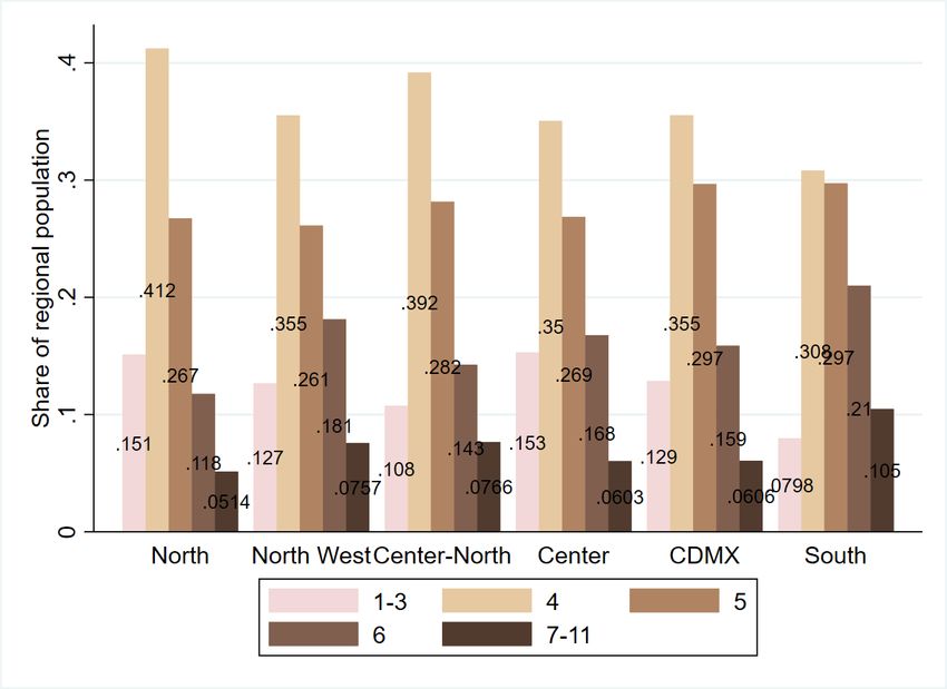
A PREPRINT - M AY 9, 2020

Introduction

The analysis of the differences in socioeconomic outcomes by skin tone and race has been a topic of concern in
economics since the middle of the XXth century (Myrdal, 1962). The research, focused in the United States, has
identified the persistence of gaps in the outcomes reached by individuals of different skin tones and races. In particular,
the African-American population faces a disadvantage compare to the white population (Corcoran et al., 1992; Darity,
Guilkey and Winfrey, 1996; Bayer and Charles, 2018; Heckman, Lyons and Todd, 2000; Neal, 2004; Bhattacharya and
Mazumder, 2011; Mazumder, 2014; Chetty et al., 2019). Albeit most of these literature has focused on the national
level, several studies such as Cutler and Glaeser (1997) and Chetty et al. (2019) have focused on the relationship
between regional variance and racial disparities, identifying a compounding effect between the two. This means that the
gap between white and black individuals is larger in communities with less resources compared to the gap observed in
more affluent communities.

In the Mexican case, albeit the study of the association between skin tones and socioeconomic status is not new
(Navarrete, 2016; Flores and Telles, 2012; Telles, 2014; Villarreal, 2010; Aguilar, 2011, 2013). there has been a
recent surge in the research in economics on the topic. Starting with the seminal audit study by Arceo-Gómez and
Campos-Vázquez (2014) on the effects of skin tone in callbacks in the labor market, the literature has grew, obtaining a
series of results on the relationship between skin tone and economic outcomes.

The first result is that individuals with darker skin tones are treated less favorably by their peers than their counterparts
with lighter skin tones. This is reported both in survey data (Aguilar, 2013) and by different experimental designs
(Aguilar, 2011; Martínez-Gutiérrez, 2019). In the case of the latter literature, Aguilar (2011) analyses if the skin
tone of political candidates affects the intention to vote of the electorate. The author identifies that darker skin
tones tend to be associated with less favorable traits with respect to those associaated with a white skin tone. This
affects the intention to vote of the electorate in favor of white skinned candidates. Martínez-Gutiérrez (2019) studies
the effects of skin tone discrimination on financial access. The author identifies that individuals with darker skin
tones receive less information and receive a ruder treatment by the bank executives than individuals with light skin tones.

In the labor market, this difference in treatment translates into different callback rates depending on the skin tone of the
person. The audit studies by Arceo-Gómez and Campos-Vázquez (2014, 2019) identify that women with darker skin
tones tend to receive less callbacks than their lighter skin tone peers. Moreover, Arceo-Gómez and Campos-Vázquez
(2019) identify that by explicitly listing a series of desired physical properties in the applicants for a vacancy, employers
reduce their searching costs. This generates an incentive for firms to be explicitly discriminatory against dark skinned
women. Related to this preference for light skinned women, Campos-Vázquez (2020) analyzes the relationship between
the price of female escort services and the physical characteristics of the service provider. The author finds a positive
correlation between both elements, suggesting that white or whiter women are deemed more desirable.

                                                             2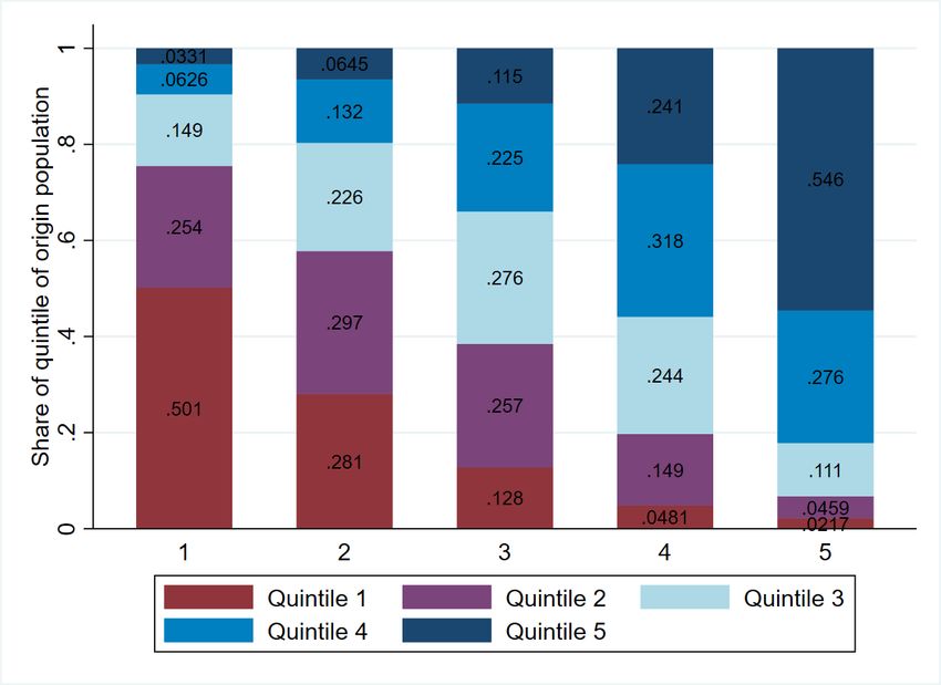
A PREPRINT - M AY 9, 2020

It is worth noting, however, that although dark skinned persons from both sexes report to be treated less fairly than
their lighter skinned counterparts (Aguilar, 2011, 2013; Martínez-Gutiérrez, 2019), the effects on the labor market
are only observed in the case of women (Arceo-Gómez and Campos-Vázquez, 2014, 2019). As the experiment
by Campos-Vázquez and Medina-Cortina (2018) shows, this has been internalized by middle school teenagers.
The authors analyze the effects of making salient the differences in social recognition between light and dark skin
toned persons on test performance and aspirations. They find that making salient the disparities in outcomes by
skin color diminish the aspirations and performance of dark skinned teenagers, the effect being driven by the female ones.

The skin tone gradient is also observable in long run life outcomes. Flores and Telles (2012); Telles (2014); Villarreal
(2010) identify that individuals with darker skill tones tend to have a lower educational attainment compared to their
lighter skin tone peers. In terms of socioeconomic status, Campos-Vázquez and Medina-Cortina (2019) identify that
upward mobility rates in terms of ranks of the socioeconomic status distribution are lower for dark skin individuals
than for white skin individuals. This occurs due to differences in the steady states to which individuals of each skin
tone are converging and not by differences in the rank correlation between origin and current position. We provided
evidence in the same direction in a previous paper (Vélez-Grajales, Monroy-Gómez-Franco and Yalonetzky, 2018).
Particularly, we identified that persistence rates at the bottom of the socioeconomic status distribution are higher for
dark skinned persons than for white individuals in the distribution. At the same time, persistence rates at the top of the
socioeconomic distribution are larger for lighter skin tone individuals than for the rest of the population. Together, both
results suggest that light skinned individuals have an advantage over dark skinned individuals in terms of moving
upwards and staying at the top of the socioeconomic distribution.

However, it is worth noting that all these results are unable to capture any variation across Mexican regions. By
design, the experimental evidence (Aguilar, 2011; Arceo-Gómez and Campos-Vázquez, 2014; Campos-Vázquez
and Medina-Cortina, 2018; Arceo-Gómez and Campos-Vázquez, 2019) can only be generalized to populations that
are at least similar to the specific sample who participated in the experiment. In the case of the papers that employ
survey information (Aguilar, 2013; Flores and Telles, 2012; Telles, 2014; Villarreal, 2010; Campos-Vázquez and
Medina-Cortina, 2019; Vélez-Grajales, Monroy-Gómez-Franco and Yalonetzky, 2018), all the surveys are only
representative at the national level. Thus, this body of research is unable to disentangle the compounding effect of
regional differences and skin color identified in other countries (Cutler and Glaeser, 1997; Chetty et al., 2019).

This limitation is important, as recent work shows that there is a substantial amount of regional variation in terms of
social mobility across Mexican regions (Monroy-Gómez-Franco and Corak, 2019; Delajara, Campos-Vázquez and
Vélez-Grajales, 2020; Orozco-Corona et al., 2019). In particular, the literature identifies that individuals with origins in
the south region of the country experience lower upward mobility rates and converge to a lower steady state that those
with origins in any other region of the country. If the skin tones do not distribute at random across the Mexican regions,
then estimates at the national level will be biased, as the skin tone effect is confounded with the regional effect.

                                                             3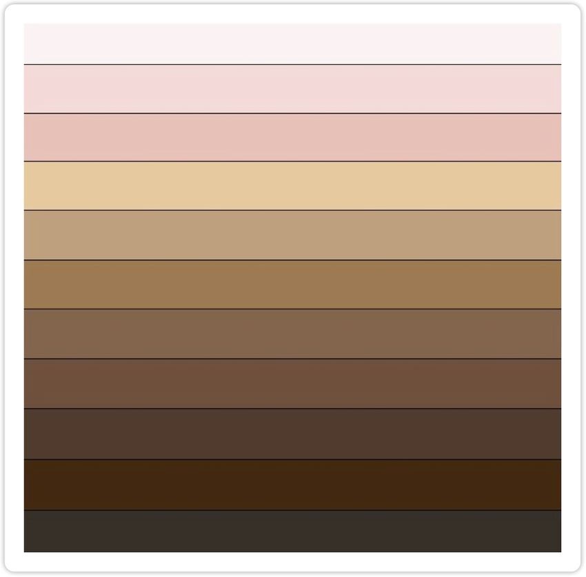
A PREPRINT - M AY 9, 2020

Our objective in this paper is to address this problem by employing a newly available data set that has information
on skin tone and is representative at the regional level. This allows us to track the movements of individuals with
the different skin tones but from the same region of origin, thus allowing us to separate the skin tone effect from
the regional one. If differences in intergenerational persistence among persons of different skin tones are constant
across regions, this would suggest a constant advantage provided by light skin tone. Otherwise, the evidence would be
suggestive of different intensities in treatment at the regional level.

Data

Most of the research on social mobility relies on the existence of panel data3 which is not always available in developing
countries. This happens to be the case of Mexico, country for which there is no long run panel data base suitable to be
employed in the study of social mobility. As an alternative, cross sectional surveys with retrospective information have
been used to recover information on the origins of the respondents. Our data source in this paper, the Encuesta ESRU
de Movilidad Social en México 2017 4 undertaken by the Centro de Estudios Espinosa Yglesias, has this characteristic.

ESRU-EMOVI 2017 is a probabilistic national and regionally representative sample of the Mexican non-institutionalized
men and women population between 25 and 64 years old. Respondents are randomly selected from the household
members within the age range, regardless of their relationship with the household head. The total sample size is of
17,655 households, and the weights5 are constructed to bring the sample distribution in accordance to the national
population. An innovation of this data set with respect to previous ones is that the sample is also representative at
the regional level, dividing the Mexican territory into five regions and an oversample of the Mexico City (CDMX)
population that allows to analyze it separately6 . The regionalization of the country was based on the similarities across
states in terms of employment and output composition.

The survey has information on educational attainment, occupational characteristics and status of the respondent and
her parents. It also contains information on a series of household assets for both the current household and the one
inhabited by the respondent at 14 years old. Crucially for our analysis, the survey includes information on the skin tone
of the respondent. This information is self-reported by the interviewee, who is asked to declare to which tone from
those in a color palette the tone of the inside part of her forearm is closest to7 .

   3
      see for instance Solon (1992); Chetty et al. (2015, 2019); Corak (2019).
   4
      ESRU Survey on Social Mobility in Mexico 2017
    5
      The weights are the inverse of the probability of selecting each household into the survey.
    6
      The North region consists of Baja California, Sonora, Chihuahua, Coahuila, Nuevo León and Tamaulipas; North West consists
of Baja California Sur, Sinaloa, Nayarit, Durango and Zacatecas; the Center North region consists of Jalisco, Aguascalientes, Colima,
Michoacán and San Luis Potosí; the Center region is formed by Guanajuato, Querétaro, Hidalgo, Estado de México, Morelos,
Tlaxcala,and Puebla; the South region is formed by Guerrero, Oaxaca, Chiapas, Veracruz, Tabasco, Campeche, Yucatán and Quintana
Roo. Mexico City is analyzed as a region of its own.
    7
      The tone palette is the one designed by Telles (2014) for the Project on Ethnicity and Race in Latin America (PERLA). It
consists of 11 tonalities deemed to be representative of the different skin tones present in Latin America. The tone at the beginning
of the scale (tone 1) is the lightest skin tone, whereas tone 11 corresponds to the darkest skin tone. The palette is showed in figure 9
in the appendix.

                                                                   4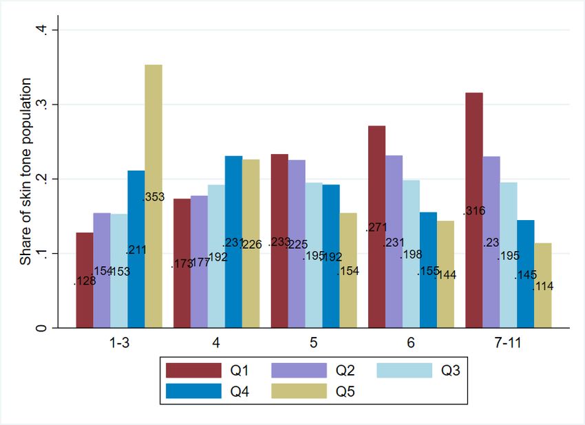
A PREPRINT - M AY 9, 2020

We recognize that retrospective information is not a direct equivalent to panel data, as it suffers from recall bias that by
definition is a function of the distance between the moment when the information is collected and the reference point
in the life of the person. EMOVI 2017 seeks to minimize this source of bias by setting the reference point for the
respondent at 14 years old. Recent research shows that autobiographical events occurred during adolescence tend to
remembered more frequently than those occurred at other life stages (Rubin and Schulkind, 1997; Koppel and Berntsen,
2016; Murre et al., 2013; Janssen, Chessa and Murre, 2007; Janssen and Murre, 2008; Maki et al., 2013; Wolf and
Zimprich, 2016; Conway et al., 2005). Hence the rationale of selecting 14 years old as the reference point for the
individual. With the same objective, the survey avoids asking too detailed questions about parental income or wealth,
and concentrates in asking the individuals to describe the living conditions of their households of origin in terms of
ownership of durable goods and household assets.

In table 1, we show the composition of the sample at the national level, and how it distributes across the six regions. As
it is possible to observe, the Mexican population is heavily concentrated in the center, CDMX and south regions of the
country. This biases the distribution of most variables, such as the female share of the population, the urban population
and the cohort composition. In the case of the indigenous population, more than half of the national indigenous
population is concentrated in the south. In terms of the skin tone distribution, it is also clear that individuals with darker
skin tones are heavily concentrated in the south (32% of the total dark skin population), and in the center regions (41%
of the total dark skin population).

                                                              5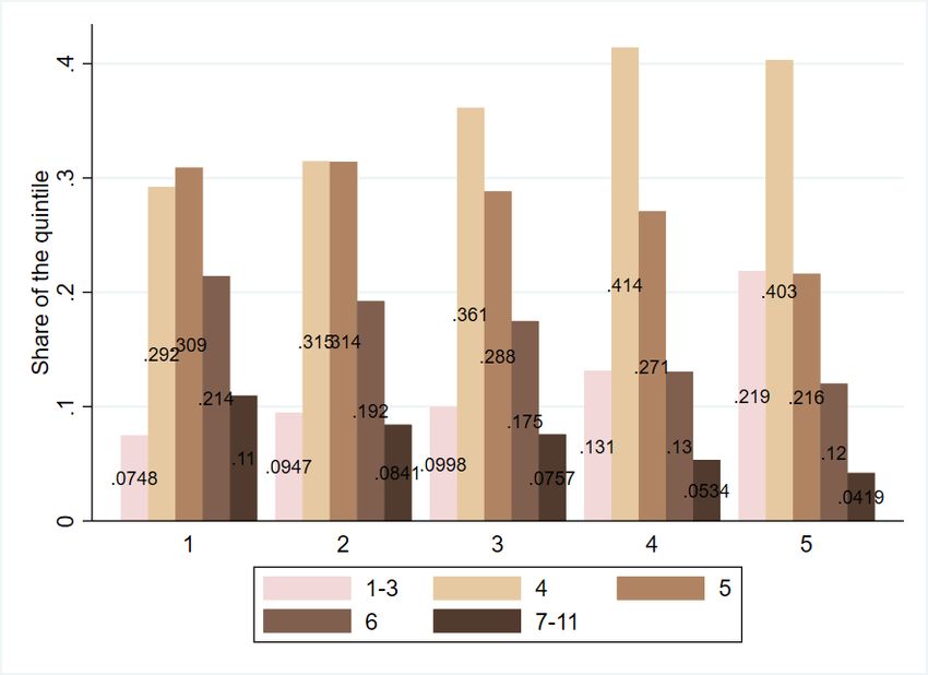
A PREPRINT - M AY 9, 2020

                                             Table 1: Descriptive Statistics
        Variable         National     North   North-West Center-North Center                      Mexico City       South
       Indigenous         12.3%        5.7%       2.1%             7.1%      33.1%|                  6.3%           56.8%
         Urban            66.4&       19.0%      5.5%             13.5%      28.9%                  16.7%           16.4%
                                            Skin tone (PERLA complete)
             1            0.7%        14.2%      6.2%             24.8%      31.2%                     8.6%         15.1%
             2            4.1%        20.8%      8.1%             11.3%      32.2%                    12.4%         15.2%
             3            7.5%        17.5%      7.3%             12.2%      34.8%                    11.8%         16.4%
             4            35.6%       17.4%      7.3%             15.9%      26.8%                    11.3%         21.3%
             5            28.0%       14.4%      6.8%             14.5%      26.1%                    12.0%         26.1%
             6            16.7%       10.6%      7.9%             12.3%      27.4%                    10.8%         31.0%
             7            4.2%        10.3%      9.0%             14.4%      23.2%                     9.7%         33.3%
             8            2.0%         8.8%       6.3%            15.2%      23.7%                     9.6%         36.3%
             9            0.7%        11.2%      3.6%             22.2%      18.1%                     6.9%         38.0%
            10            0.3%        24.4%      3.0%             10.3%       5.1%                    12.0%         45.2%
            11            0.1%         7.3%       9.6%             5.9%      41.4%                     3.8%         32.1%
                                                Skin tone (Collapsed)
      1-3 (lightest)      12.3%       18.4%      7.5%             12.6%      33.8%                    11.8%         15.9%
             4            35.6%       17.4%      7.3%             15.9%      26.8%                    11.3%         21.3%
             5            28.0%       14.4%      6.8%             14.5%      26.1%                    12.0%         31.0%
             6            16.7%       10.6%      7.9%             12.3%      27.4%                    10.8%         31.1%
      7-11 (darkest)      7.3%        10.5%      7.5%             15.1%      22.4%                     9.4%         35.1%
        Migrant           12.8%        4.1%      10.1%            12.2%      18.5%                    31.3%         23.7%
         Female           52.8%       14.7%      7.2%             14.8%      26.8%                    11.8%         24.8%
                                                       Cohort
          50-64           24.0%       14.1%      7.7%             15.6%      24.5%                    14.0%         24.2%
          40-50           26.3%       15.0%      7.7%             14.1%      27.3%                    10.5%         25.4%
          30-40           29.4%       15.2%      6.9%             14.9%      27.9%                    10.1%         24.9%
          24-30           20.3%       15.8%      6.8%             13.0%      29.5%                    11.1%         23.7%
                                                   Region of origin
         North             15%           -          -                -          -                        -             -
       North-West         7.3%           -          -                -          -                        -             -
      Center-North        14.4%          -          -                -          -                        -             -
         Center           27.3%          -          -                -          -                        -             -
      Mexico City         11.4%          -          -                -          -                        -             -
         South            24.6%          -          -                -          -                        -             -
                                           Regional population distribution
       Sample size        16,374      2,527      2,094            2,815       2,395                   2,638          3,905
    Note: The North region consists of Baja California, Sonora, Chihuahua, Coahuila, Nuevo León and Tamaulipas; North
    West consists of Baja California Sur, Sinaloa, Nayarit, Durango and Zacatecas; the Center North region is form by Jalisco,
    Aguascalientes, Colima, Michoacán and San Luis Potosí; the Center region is formed by Guanajuato, Querétaro, Hidalgo,
    Estado de México, Morelos, Tlaxcala, and Puebla; Mexico City is analyzed independently; the South region is formed by
    Guerrero, Oaxaca, Chiapas, Veracruz, Tabasco, Campeche, Yucatán y Quintana Roo. Indigenous represents the population
    who had at least one parent that speaks an indigenous tongue. The urban population are the persons that consider that
    their community of origin had more than 2,500 inhabitants. Migrant population is defined as those that currently inhabit a
    region different from the one they inhabited at 14 years old. The national column represents the share of the Mexican
    population from 24-65 years old. Each regional column shows the percentage of the national population that has the
    indicated characteristic and and has its origin in the indicated region. It sums 100% horizontally. Analytic weights are
    employed.

In figure 1 we show the internal skin tone composition of the six regions (panel 1a) and how the skin tones distribute
among the regions (panel 1b). In the case of the internal distributions, it is notable the similarity in terms of the skin
tone composition of each region. In all the regions, the majority of the population is concentrated in tones 4 and 5 of the
PERLA scale. As expected, the share of individuals with skin tones 7-11 is larger in the south than in other regions.

                                                                6
A PREPRINT - M AY 9, 2020
In the case of the lightest skin tones, they constitute a minority in all the regions, accounting for 15% of the regional
population in the north and the center.
Figure 1: Distribution of the Mexican population by skin tone
(a) Skin Tone composition of each region (b) Distribution of skin tones across regions
Notes: Panel a) shows the share of the regional population of each skin tone. Panel b) shows the share of the population of each skin
tone that inhabits each one of the regions. Analytic weights are employed.
Both elements, a similar internal regional composition in terms of skin tones and an unbalanced distribution of the
population of each skin tone across regions, raise the need to separate the regional effect from the skin tone effect.
These two characteristics also motivate our empirical strategy: taking into consideration the similarities of the skin tone
composition, we can compare the social mobility rates of individuals of the same region but different skin tones. At
the same time, we can compare the social mobility rates of individuals that share the same skin tone, but come from
different regions.
An element to take into account is that the sample of EMOVI 2017 is designed to be representative at the level of
the region currently inhabited, which is not necessarily the same as the region of origin. This may be a problem in
identification of the social mobility measures at the regional level, as it conflates the effects of migration with those of
the region under analysis. As a proper investigation of the determinants of migration and the differences of selection
mechanisms across regions is beyond the scope of this paper, we opt to only study the "non-migrant" population.
That is, we restrict our sample to include only those individuals who declare to inhabit in 2017 the same region they
inhabited at the reference point, i.e. when they were 14 years old.
We employ as outcome variable for our analysis an index of household assets and services for both the current and
the origin household. In order to construct the index for the household of origin we employ the set of retrospective
questions in EMOVI 2017. Said questions recover information on the characteristics of the households inhabited by the
respondent when she was 14 years old. Specifically, the assets employed to construct the index are described in table 2,
7A PREPRINT - M AY 9, 2020
and the assets employed in the construction of the index for the current household are described in table 3.
Table 2: Binary Variables for the origin household asset index
Household had a stove A household member owned the inhabited
house/apartment
Household had a washing machine Household had cable TV
Household had a refrigerator Household had clean water
Household had a television Household had a land line telephone
Household had a computer Household had electricity
Household had a DVD/VHS player Household had a microwave
A member of the household owned real Household had a vacuum cleaner
state for commercial use
A member of the household owned an auto- Household had a boiler
mobile
A member of the household had a bank ac- A member of the household had a credit
count card
There was a domestic worker employed Household was overcrowded
Source: EMOVI 2017
Asset indexes have been previously employed as proxy measures of permanent income of the household (McKenzie,
2015; Filmer and Pritchett, 2001; Wendelspiess-Chávez-Juárez, 2015) or its latent welfare (Sahn and Stifel, 2000,
2003; Bhorat and van der Westhuizen, 2013) in the absence of other types of data such as income or expenditures.
More recently, they have been employed in the estimation of social mobility (Torche, 2015; Campos-Vázquez and
Medina-Cortina, 2019; Vélez-Grajales, Stabridis and Minor-Campa, 2018), as they represent an aggregate measure of
the economic resources available in both the origin and the current household. In general, they have been found to be
strongly correlated with measures of long run outcomes of the household, and less so with variables susceptible to be
affected by short run variations (Filmer and Scott, 2012). This highlights their suitability for social mobility analysis.
Table 3: Binary Variables for the current household asset index
Household has a computer Household has a boiler
Household has a washing machine Household has internet service
Household has a DVD Household has clean water access
Household has an automobile Household has cable TV service
Household has a boiler Household has land floor
Household has a microwave Household has a bank account
Household has a stove Household has a work vehicle
Household has a domestic employee Household has a credit card
Either you or your partner/spouse own an- Either you or your partner/spouse own real
other house/apartment state for commercial use
Either you or your partner/spouse own land Either you or your partner/spouse own land
for agricultural uses for non-agricultural uses
Household has earth floor Household hires a domestic worker
A household member owns an automobile Household is overcrowded
Source: EMOVI 2017
As the survey only records the possession of each asset in tables 2 and 3, the corresponding variables are binary
variables. This makes Multiple Correspondence Analysis (MCA) the appropriate technique to generate the weights used
to aggregate the information provided by each variable. This sets us apart from the previous work by Campos-Vázquez
and Medina-Cortina (2019), who used Principal Component Analysis (PCA) to construct the weights that summarize
8A PREPRINT - M AY 9, 2020
the information in the assets and, in their case, years of education, into a socioeconomic index. The difference in the
choice of method to construct the asset index is that PCA requires the inclusion as of a continuous variable, as it
generates the weights assigned to each variable by calculating Euclidean distances. As we do not have said type of
variable, we rely on frequencies to construct the weights, which is the process behind MCA.
The selection of which variables were to be included in the index was done by discarding those that had an associated
weight without economic sense. By economic sense, we mean that the sign of the weight assigned to each asset has
to be positive in the case of goods, and negative in the case of bads. This approach, suggested by Wittenberg and
Leibbrandt (2017) guarantees both the statistical and economic consistency of the ranking produced by the household
assets index. However, it also leads to different sets of assets being employed in the construction of the current and the
origin household indexes. This is not a problem as long as the analysis is restrict to relative social mobility, as said
type of analysis only asks the indexes to produce consistent rankings of the individuals according to a socioeconomic
outcome variable.
Method of Analysis
The first step in our analysis is to construct the distributions along which the movements of the individuals are going
to be tracked. As the sample is composed by individuals between 25 to 64 years old, a first step is to separate them
into different cohorts in order to enhance the comparability on mobility rates. Thus, we divide the sample into four
cohorts: 24 to 30 years old, 30 to 40 years old, 40 to 50 years old and 50 to 64 years old. By narrowing the age span of
each cohort, we make both the current stage of the life cycle and the year in which the reference point occurred more
homogeneous across individuals. Then, for each cohort, we produce a national ranking of all individuals of each cohort
by considering all regions together. This allows to compare the mobility rates of individuals from each different region,
as the movements are defined on the same distribution. After this process we end up with eight household rankings, one
for the origin household and another for the current household of each one of the four cohorts.
As described above, the household assets index allows us to rank individuals according to the amount of resources they
have8 . This sets a natural context for the use of rank-based relative mobility measures, which, as Nybom and Stuhler
(2017) show, are less subject to life-cycle bias. Among these measures, we employ the rank-rank correlation as our
main tool of analysis, as it is closely linked to the basic model of intergenerational transmission of status developed by
Becker and Tomes (1986).
Specifically, let Rt 1,i.c be the percentile in which the origin household i of cohort c was located in the corresponding
origin distribution, and Rt,i,c is the percentile where the respondents household lies in the corresponding current
household distribution. ⇢s 2 [0, 1] is the skin tone persistence rate, that is, the rate of transmission of the origin rank
into the current rank. In the same vein, ↵s 2 [0, 1] is the skin tone specific intercept, which, following Chetty et al.
8
Or had, in the case of the case of the origin household
9A PREPRINT - M AY 9, 2020
(2014, 2015) interpretation, captures the absolute mobility of the individuals starting from the lowest percentile in the
origin distribution.
Rt,i,c = ↵s + ⇢s Rt 1,i,c + ui,t,c (1)
By generating the rankings for each cohort separately, our main specification (equation ) is equivalent to estimating
the persistence rate including cohort specific controls. Thus, the pooled estimate will provide an average of the
persistence rates observed in all cohorts. Assuming that ui,t,c is a random shock orthogonal to the ranks, and has mean
of E[ui,t,c ] = 0 we can estimate the mean rank by skin color-cohort as:
R̄i,t = ↵s + ⇢s R̄i,t 1 (2)
Solving in iterative fashion, we get for period t + k
R̄i,t+k = ↵[1 + ⇢s + ⇢2s + ... + ⇢ks 1
] + ⇢ks R̄i,t+k (3)
1 ⇢ks
=↵ + ⇢ks R̄i,t (4)
1 ⇢s
Since ⇢s,c 2 [0, 1], as k ! 1 the previous expression becomes
↵s,c
R̄sss = (5)
1 ⇢s,c
In equation 5, R̄sss is the steady state for the individuals of group of skin tone s in cohort c. Notice that said
steady state depends of , ↵s,c and ⇢s,c . Thus, any difference in the steady states across skin tones and cohorts is
due to either one of those two factors. We then define the difference in steady states between skin tone s and skin tone z as
R̄jss = R̄sss R̄zss (6)
As Chetty et al. (2019) state, this leads to three possible cases:
• Same rate of persistence and same absolute mobility across skin tones: In this case there would be no difference
in the steady states to which the different skin tones of every cohort converge, that is R̄jss = 0
• Same rate of persistence, different absolute mobility: This case implies that although the individuals from
different skin colors are converging at the same speed towards their steady state rank, the rank to which they
are converging is different due to the differences in the absolute mobility achieved by those at the bottom of
10A PREPRINT - M AY 9, 2020
the distribution. In this case
↵j
R̄jss = (7)
1 ⇢
in which ↵s,j = ↵s,j ↵z,j
• General case: The most general case assumes different rates of persistence and different rates of absolute
mobility from the bottom. Thus
ss ↵s ↵z
R̄j,c = (8)
1 ⇢s 1 ⇢z
Notice however, that in all three cases the rate of persistence and the absolute mobility from the bottom are estimated for
the national population of each skin tone. This implies assuming a homogeneous distribution of skin tones across the
country, which, as shown by figure 1b, is not a realistic assumption for the Mexican case. For this reason, we estimate
the steady states for each skin tone for each region.
ss ↵s,r
R̄s,r = (9)
1 ⇢s,r
where the subscript r indicates the region for which the steady state is estimated. If the regional differences do not play
a role, it is expected that the steady state of the same skin color will be constant across regions for individuals of the
same generation. If, however, the regional differences are generating part of the effect attributed to skin tone, we would
expect to see different steady states by region for individuals with the same skin tone.
Although rank-rank correlations provide summary measures on the rate of position persistence, they do not capture
the existence of differences in said rates at different points of the socioeconomic distribution. To do so, we estimate
transition matrices, focusing particularly at the extremes of the distribution. Specifically, we estimate skin tone specific
transition matrices at the national and regional level. In order to validate our data, we also estimate a transition matrix
for the total population and compare it with the patterns observed in previous studies. Formally, let ⌦(t) be the position
of individual t inside the national distribution of the outcome variable, and ⌦(t) 2 [⌦min , ⌦max ] where ⌦min = 1 and
⌦max = 5 are the minimum and the maximum possible positions. Then, define Zi|j as the transition probability in the
national distribution of the respondent being in position i given that the origin household was in position j.
Ni|j
Zi|j ⌘ P r[⌦(s) = i|⌦(o) = j] ⌘ (10)
Nj
With these transition probabilities, we construct the national transition matrices by skin tone, which describes the
mobility patterns of the individuals from each skin tone along the national distribution. Formally, let Mo,p
N
be said
matrix defined as
2 3
Z1|1 ... Z5|1
6 . .. .. 7
N
Mo,p ⌘6 . 7 (11)
4 . . . 5
Z1|5 ... Z5|5
11A PREPRINT - M AY 9, 2020
Results
We start with an overall analysis of the mobility patterns at the national level. We seek to replicate the findings of
previous literature that identify a high degree of persistence at the extremes of the distribution. (see Campos-Vázquez
and Medina-Cortina (2019); Vélez-Grajales, Campos-Vázquez and Huerta-Wong. (2014); Monroy-Gómez-Franco,
Vélez-Grajales and Yalonetzky (2018)).
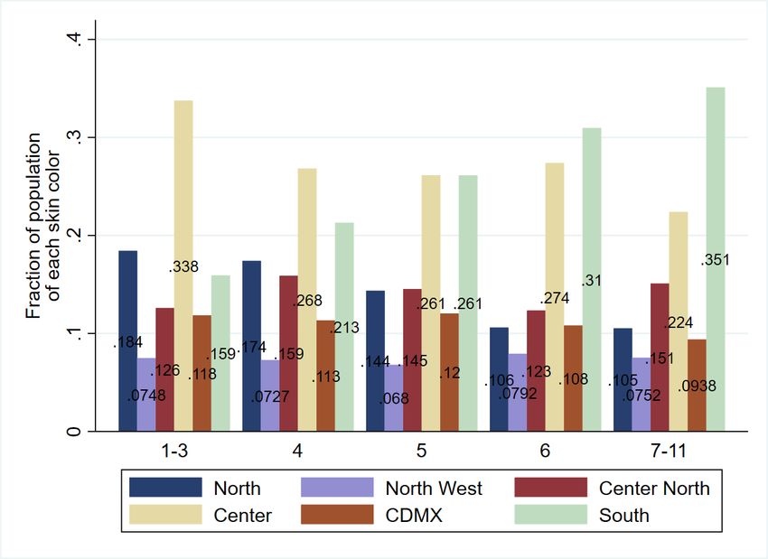
Figure 2: National mobility patterns.
(a) National Transition Matrix (b) National Rank-Rank Correlation
Note: The regression line in figure 2b is estimated over the underlying data, and not on the binned data presented in the figure.
Analytic weights are employed.
Source: EMOVI 2017
Our findings coincide with what has been identified in previous literature. As figure 2b describes, there are high degrees
of rank persistence at the extremes of the socioeconomic distribution. That is, we observe high persistence rates (50%
of those who begin at an specific quintile remain there in adulthood) both at the bottom and at the top 20% of the
Mexican socioeconomic distribution. And in the case of the general distribution, we observe also a high persistence
rate, described by the rank-rank correlation.
We are also able to replicate the previous finding in the literature that identifies that, at the national level, persons with
lighter skin tones experience higher upward mobility starting from the first quintile of the distribution (see figure 3a). In
the same vein, it is possible to observe that the point estimate of the darker skin tones correspond to the lowest upward
mobility rates. Similarly, we observe that persons with lighter skin tones experience lower downward mobility rates
from the top of the distribution, compared with the rest of skin tones. The highest downward mobility rates correspond
to individuals with the darkest skin tones (see figure 3b).
We are also interested in analyzing the composition of the different quintiles in terms of skin tone and in identifying
how the individuals that share a skin tone distribute themselves across the socioeconomic scale. Figure 4a shows the
12A PREPRINT - M AY 9, 2020
Figure 3: Upward and downward social mobility by skin tone
(a) Upward mobility from the bottom (b) Downward mobility from the top
Notes: Panel a) shows the share of individuals whose origin household belongs to the bottom quintile of the distribution and their
current household belongs to a different quintile. Panel b) shows the share of individuals whose origin household belongs to the top
quintile of the distribution and their current household belongs to a different quintile.
Source: EMOVI 2017
share of the population from each skin tone according to the quintile to which their household of origin belonged.
Around a third of the population with the lightest skin tones comes from the top 20% of the distribution, where only
12% come from the bottom quintile. The reverse pattern is observed for the persons with the darkest skin tone: about a
third of that population comes from households that were part of the bottom quintile, whereas only 11% comes from
households at the top 20%.
As Monroy-Gómez-Franco and Corak (2019); Orozco-Corona et al. (2019) show, the bottom quintile of origin is
concentrated in the south region of the country. This, together with the information on figure 1b, suggests that the
omission of the regional dimension might lead to missatribute the regional effect to the skin tone one. Figure 1a shows
that with respect to the the total population at each quintile, the skin tones are also not evenly distributed. Individuals of
the lightest skin tone represent around a third of those located at the top of the distribution. The same group represents
less than 10% of those at the bottom quintile. The reverse pattern is observed for those of the darkest skin tones. Said
group represents less than 5% of those located at the top of the population, and they represent 11% of those located at
the bottom quintile.
We then proceed to incorporate regional differences into our analysis. Our first approach is to estimate the upward and
downward mobility rates for each skin tone, analyzing separately each region of origin. This is equivalent to condition
the mobility rate by region of origin, thus allows to observe if any difference by skin tone persists when individuals
from the same region of origin are compared between themselves.
13A PREPRINT - M AY 9, 2020
Figure 4: Skin tone distributions.
(a) Skin tone distributions across quintiles (b) Composition of each quintile by skin tone
Notes: Panel a) shows the share of individuals whose origin household belongs to the bottom quintile of the distribution and their
current household belongs to a different quintile. Panel b) shows the share of individuals whose origin household belongs to the top
quintile of the distribution and their current household belongs to a different quintile.
Source: EMOVI 2017
For the case of upward mobility from the bottom of the distribution, figure 5 shows that, with the exception of the south,
there are no statistically significant differences among the rates of mobility experienced by the different skin tones.
However, in the case of the south, there is a clear difference in the upward mobility rates between the lightest and the
darkest skin tone, in favor of the former. As the region concentrates a large part of the population with this skin tone,
the lower mobility rates experienced in this region bias downward the national estimate.
With respect to downward mobility from the top quintile, the previous pattern is not observed, as figure 6 shows. In this
case, in the North, CDMX and South regions the individuals with the darkest skin tones with origin at the top 20% of
the population face larger rates of downward mobility than individuals from the same regions and starting position
but with the lightest skin tone. However, for the other three regions, the difference between tones is not statistically
significant.
Both the estimates of upward and downward mobility suggest that the patterns observed so clearly at the national level
are less clear once each region is analyzed separately. Albeit in most cases the point estimates follow the same patterns
as the national ones, the differences across skin tones are less stark and in most cases are not statistically significant.
However, as it is possible to notice from the confidence intervals, the estimations are not very precise. This is a natural
consequence of the non parametric approach followed in the estimation process and of the finesse of the partitions
employed, which reduce substantially the number of observations per cell.
In order to confirm these findings, we proceed to estimate the rank-rank correlations by skin tone and region, as the
parametric estimation is a less data demanding method. In figure 7 we compare the slope estimates for the same skin
14A PREPRINT - M AY 9, 2020
Figure 5: Upward mobility rates from the bottom quintile
(a) North region (b) North West region
(c) Center North region (d) Center region
(e) CDMX (f) South region
The red bars indicate the 95% bootstrap confidence intervals. Analytic weights are employed.
15A PREPRINT - M AY 9, 2020
Figure 6: Downward mobility rates from the top quintile
(a) Region North (b) Region North West
(c) Region Center North (d) Region Center
(e) CDMX (f) Region South
The red bars indicate the 95% bootstrap confidence intervals. Analytic weights are employed.
16A PREPRINT - M AY 9, 2020
Figure 7: Persistence coefficients across Mexican regions
(a) Persistence coefficient for tones 1-3 (b) Persistence coefficient for tone 4
(c) Persistence coefficient for tone 5 (d) Persistence coefficient for tone 6
(e) Persistence coefficient for tones 7-11
tone across the different regions9 . For all skin tones it is possible to note that there are no statistically significant
differences across the regions in terms of the slope estimates. Assuming that these persistence patterns are constant
through time, this would imply that the rates of convergence to the corresponding steady state of each skin color do not
vary by region. However, this does not rules out the existence of regional differences in the steady states to which each
skin tone is converging.
In order to check for this, we estimate the steady states to which each skin tone-region group would converge assuming
that the estimated slopes are constant through time using equation 5. Our results, presented in figure 8, show that, with
9
The complete regression tables are presented in the appendix in tables 5-10
17A PREPRINT - M AY 9, 2020
the exemption of the North West and Center North regions, there is a gap between the steady state to which persons
with the lightest skin tones are converging and the one that corresponds to individuals with the darkest skin tones.
However, the size of the gaps varies substantially across regions. For example, in the case of the CDMX, the difference
between the point estimates is of 17 points, between percentile 80 for the lightest skin tones and percentile 67 for the
darkest skin tone. In comparison, in the Center Region, the lightest skin tone would be converging to the 70 percentile
of the national distribution, while the darkest skin tone would converge to the 40 percentile.
This heterogeneity across steady states is also present when we compare across regions for the same skin tone. while in
CDMX the lightest skin tone is converging to percentile 80 of the national distribution, the population of the same skin
tone but with origins in the south region is converging to the median of the national distribution. In this case, the gap
between individuals of the same skin tone but different regions is larger than the gap between individuals of different
tones but the same region, as exemplified lines above. The heterogeneity is also present in the darkest skin tones, being
more extreme in that case. While in CDMX the darkest skin tone is converging to the 70 percentile of the national
distribution, in the south the same skin tone is converging to the 25 percentile.
Jointly with the distribution of skin tones in the country, the differences in the steady state ranks suggest that the gaps in
relative social mobility between skin tones are heavily influenced by the regional heterogeneity observed in Mexico.
Our analysis shows that once information is conditioned by region of origin, the gaps are less wide than the national
data would suggest. However, as before, the number of partitions of the data diminishes the precision of the estimations.
We then proceed to estimate the conditional rank-rank correlation for the whole sample, introducing different controls
in a progressive manner. We are particularly interested in analysing if the introduction of the regional controls leads to a
fall in the absolute value of the coefficients associated with the skin tone. This exercise is showed in table 4.
18A PREPRINT - M AY 9, 2020
Figure 8: Steady states by region
(a) Region North (b) Region North West
(c) Region Center North (d) Region Center
(e) CDMX (f) Region South
The red bars indicate the 95% bootstrap confidence intervals. Analytic weights are employed.
19A PREPRINT - M AY 9, 2020
Table 4: Conditional rank-rank correlation
Variable Model 1 Model 2 Model 3 Model 4 Model 5 Model 6 Model 7
Parental rank 0.613*** 0.613*** 0.588*** 0.548*** 0.466*** 0.445*** 0.516***
(0.00919) (0.00924) (0.00949) (0.0353) (0.0351) (0.0435) (0.0450)
Skin tones 1-3 10.92*** 6.999** 4.444* 6.508** 5.454*
(1.329) (2.736) (2.665) (2.844) (2.865)
Skin tone 4 6.269*** 4.184** 2.866 1.790 0.997
(1.149) (2.015) (1.910) (1.869) (1.865)
Skin tone 5 2.310* 1.516 0.494 2.229 1.969
(1.199) (2.056) (1.956) (1.887) (1.880)
Skin tone 6 0.267 -1.184 -1.915 -0.830 -0.903
(1.266) (2.155) (2.076) (2.045) (2.036)
North region 11.12*** 13.85*** 20.75***
(0.798) (3.607) (3.867)
North West region 10.49*** 17.04*** 23.07***
(0.855) (3.201) (3.348)
Center North region 9.347*** 13.31*** 16.93***
(0.800) (2.709) (2.838)
Center region 10.57*** 9.069** 9.561**
(0.986) (3.582) (3.772)
CDMX 16.99*** 20.87*** 23.45***
(0.804) (2.834) (3.098)
Tones 1-3 ⇥ Origin rank 0.0794* 0.114*** 0.140*** 0.141***
(0.0447) (0.0441) (0.0533) (0.0529)
Tone 4 ⇥ Origin rank 0.0498 0.0667* 0.0749 0.0817*
(0.0383) (0.0372) (0.0466) (0.0463)
Tone 5 ⇥ Origin rank 0.0228 0.0315 0.0675 0.0704
(0.0396) (0.0386) (0.0483) (0.0479)
Tone 6 ⇥ Origin rank 0.0371 0.0438 0.0656 0.0623
(0.0421) (0.0413) (0.0515) (0.0509)
North region ⇥ Origin rank -0.158***
(0.0268)
North West region ⇥ Origin rank -0.182***
(0.0300)
North Center region ⇥ Origin rank -0.110***
(0.0265)
Center region ⇥ Origin rank -0.0398
(0.0333)
CDMX ⇥ Origin rank -0.0846***
(0.0280)
Female -2.769*** -3.430*** -3.449*** -3.642*** -3.625*** -3.601***
(0.608) (0.602) (0.602) (0.587) (0.580) (0.578)
20A PREPRINT - M AY 9, 2020
Conditional rank-rank correlation (continued)
Variable Model 1 Model 2 Model 3 Model 4 Model 5 Model 6 Model 7
Tone 1-3 ⇥ North -4.430 -2.651
(4.381) (4.295)
Tone 1-3 ⇥ North West -10.60** -7.950*
(4.229) (4.166)
Tone 1-3 ⇥ Center North -8.053** -6.651*
(3.762) (3.751)
Tone 1-3 ⇥ Center 0.190 0.501
(4.609) (4.665)
Tone 1-3 ⇥ CDMX -6.479* -5.267
(3.836) (3.823)
Tone 4 ⇥ North -0.113 0.391
(3.841) (3.771)
Tone 4 ⇥ North West -2.095 -0.565
(3.517) (3.432)
Tone 4 ⇥ Center North -2.049 -1.211
(3.038) (3.037)
Tone 4 ⇥ Center 4.813 4.732
(3.922) (3.946)
Tone 4 ⇥ CDMX -1.397 -0.951
(3.143) (3.136)
Tone 5 ⇥ North -5.343 -5.664
(3.883) (3.831)
Tone 5 ⇥ North West -9.325*** -8.437**
(3.534) (3.452)
Tone 5 ⇥ Center North -4.943 -4.687
(3.090) (3.086)
Tone 5 ⇥ Center -1.579 -1.659
(4.093) (4.103)
Tone 5 ⇥ CDMX -7.529** -7.382**
(3.191) (3.173)
Tone 6 ⇥ North -3.696 -3.753
(4.152) (4.092)
Tone 6 ⇥ North West -10.56*** -9.542***
(3.767) (3.694)
Tone 6 ⇥ Center North -5.100 -4.824
(3.245) (3.247)
Tone 6 ⇥ Center 1.024 1.185
(4.282) (4.281)
Tone 6 ⇥ CDMX -2.763 -2.390
(3.428) (3.417)
Constant 19.51*** 23.12*** 17.08*** 18.66*** 13.12*** 12.91*** 10.72**
(0.561) (4.083) (4.219) (4.467) (4.354) (4.317) (4.312)
Observations 14,333 14,333 14,333 14,333 14,333 14,333 14,333
R-squared 0.409 0.413 0.427 0.427 0.454 0.456 0.460
Notes: The omitted skin tone corresponds to categories 7-11 of the PERLA scale. The omitted region corresponds to the south region. Models 2 to 7 include age and
age squared as controls. Robust standard errors in parentheses. Source: EMOVI 2017. *** pA PREPRINT - M AY 9, 2020
of the regional dummies, confirming our previous results that analyze each region separately. Our results suggest that
skin tone matters in Mexico, but less than what we originally thought so.
Notice that although the interactions between skin tones and regions are, for the most part, non statistically significant,
the interaction between light skin tone and the origin rank is statistically significant in all the models in which it is
included. This non-linearity coincides with our result from the transition matrices that showed that light skin individuals
are able to move upwards more frequently in the socioeconomic distribution, and at the same time are more able
to retain their position at the top with respect to those with the darkest skin tone. This suggests that light skin acts
in conjunction with the socioeconomic status of origin in determining the type social mobility experienced by the
individual.
It is also worthwhile to note that the interactions between the regions and the rank of the origin household are
statistically significant and in all cases have a negative sign. This implies a penalty for all individuals with origin in
the south, as they would be subject to a higher degree of rank persistence in the national distribution than individuals
coming from any other region. This is indicative of the effects that the medium run lackluster performance of the south
in terms of economic growth are having on the life prospects of the inhabitants of the region (Davalos et al., 2015;
Esquivel, 1999; Campos-Vázquez and Monroy-Gómez-Franco, 2016).
Conclusion
Our main objective in this paper was to analyze if the advantage in terms of social mobility associated to having a lighter
skin tone identified at the national scale, subsisted using more disaggregated information. Our results confirm that said
effect persists, albeit is smaller than the one identified by the previous research using information representative at the
national level (Campos-Vázquez and Medina-Cortina, 2019; Monroy-Gómez-Franco, Vélez-Grajales and Yalonetzky,
2018).
In order to be able to provide more detailed and precises analyses on the effects of skin tone stratification on social
mobility a series of data innovations are needed. The main one is the need to have a reference point for the distribution
of skin tones across regions. The lack of census data with this type of information acts as a limitation both to the
analysis of skin tone stratification in Mexico, and to the production of survey information that seeks to capture the
distribution of skin tones in the country.
It is important to emphasize that our results take as a given the current geographical distribution of skin tones. Said
distribution is the fruit of a complex process of historical development that as one of it results, has produced widely
different outcomes in terms of the economic development of Mexican regions. Our results cast a new light into
the enquiries of the literature on regional divergence, pointing out the necessity to study the role played by social
stratification by skin tone in the long run patterns of regional development in Mexico.
22A PREPRINT - M AY 9, 2020
Conflict of interest
On behalf of all authors, the corresponding author states that there is no conflict of interest
References
Aguilar, Rosario. 2011. “Social and political consequences of stereotypes related to racial phenotypes in Mexico.”
Centro de Investigación y Docencia Económicas Working Paper 230.
Aguilar, Rosario. 2013. “Los tonos de los desafíos democráticos: el color de la piel y la raza en México.” Política y
Gobierno, 25–57.
Arceo-Gómez, Eva, and Raymundo Campos-Vázquez. 2014. “Race and Marriage in the Labor Market: A Discrimi-
nation Correspondence Study in a Developing Country.” American Econommic Review, 104(5): 376–380.
Arceo-Gómez, Eva, and Raymundo Campos-Vázquez. 2019. “Double Discrimination: Is Discrimination in Job Ads
Accompanied by Discrimination in Callbacks?” Journal of Economics, Race, and Policy, 2(4): 257–268.
Bayer, Patrick, and Kerwin Kofi Charles. 2018. “Divergent Paths: A New Perspective on Earnings Differences
Between Black and White Men Since 1940.” The Quarterly Journal of Economics, 133(3): 1459–1501.
Becker, Gary S., and Nathan Tomes. 1986. “Human Capital and the rise and fall of families.” Journal of Labor
Economics, 4: 1–39.
Bhattacharya, Debopam, and Bhaskar Mazumder. 2011. “A Nonparametric Analysis of Black-White Differences
in Intergenerational Income Mobility in the United States.” Quantitative Economics, 2(3): 335–379.
Bhorat, Haroon, and Carlene van der Westhuizen. 2013. “Non-monetary dimensions of well-being in South Africa,
1993–2004: A post-apartheid dividend?” Development Southern Africa, 30(3): 295–314.
Campos-Vázquez, Raymundo. 2020. “The higher price of whiter skin: an analysis of escort services.” Applied
Economics Letters, 0(0): 1–4.
Campos-Vázquez, Raymundo, and Eduardo Medina-Cortina. 2018. “Identidad Social y Estereotipos por Color de
Piel. Aspiraciones y Desempeño en Jóvenes Mexicanos.” El Trimestre Económico, 85(1): 53–79.
Campos-Vázquez, Raymundo, and Eduardo Medina-Cortina. 2019. “Skin Color and Social Mobility: Evidence
from Mexico.” Demography, 56(1): 77–113.
Campos-Vázquez, Raymundo, and Luis Monroy-Gómez-Franco. 2016. “¿El crecimiento económico reduce la
pobreza en México?” Revista de Economí Mexicana. Anuario UNAM, 1(1): 140–185.
Chetty, Raj, Nathaniel Hendren, Maggie R. Jones, and Sonya R. Porter. 2019. “Race and Economic Opportunity
in the United States: An Intergenerational Perspective*.” The Quarterly Journal of Economics. qjz042.
Chetty, Raj, Nathaniel Hendren, Patrick Kline, and Emmanuel Saez. 2015. “Where is the Land of Opportunity?
The Geography of Intergenerational Mobility in the United States.” The Quarterly Journal of Economics, 129(4): 1553–
1623.
Chetty, Raj, Nathaniel Hendren, Patrick Kline, Emmanuel Saez, and Nicholas Turner. 2014. “Is the United States
Still a Land of Opportunity? Recent Trends in Intergenerational Mobility.” American Economic Review: Papers and
Proceedings, 104(5): 141–147.
23A PREPRINT - M AY 9, 2020
Conway, Martin A., Qi Wang, Kazunori Hanyu, and Shamsul Haque. 2005. “A Cross-Cultural Investigation of
Autobiographical Memory: On the Universality and Cultural Variation of the Reminiscence Bump.” Journal of
Cross-Cultural Psychology, 36(6): 739–749.
Corak, Miles. 2019. “The Canadian Geography of Intergenerational Income Mobility.” The Economic Journal.
Corcoran, Mary, Roger Gordon, Deborah Laren, and Gary Solon. 1992. “The Association between Men’s Eco-
nomic Status and Their Family and Community Origins.” Journal of Human Resources, 27(4): 575–601.
Cutler, David M., and Edward L. Glaeser. 1997. “Are Ghettos Good or Bad?” The Quarterly Journal of Economics,
112(3): 827–872.
Darity, William, David K. Guilkey, and William Winfrey. 1996. “Explaining Differences in Economic Performance
among Racial and Ethnic Groups in the USA: The Data Examined.” The American Journal of Economics and
Sociology, 55(4): 411–425.
Davalos, Maria E., Gerardo Esquivel, Luis Felipe López-Calva, and Carlos Rodríguez-Castelán. 2015. “Conver-
gence with Stagnation: Mexico’s Growth at the Municipal level 1990-2010.” Sobre México. Temas en economía.
Delajara, Marcelo, Raymundo Campos-Vázquez, and Roberto Vélez-Grajales. 2020. “Social Mobility in Mexico.
What Can We Learn from Its Regional Variation?” Agence Française de Développement Working Paper.
Esquivel, Gerardo. 1999. “Convergencia regional en México, 1940-1995.” El Trimestre Económico, 66(264): 725–761.
Filmer, Deon, and Kinnon Scott. 2012. “Assessing Asset Indices.” Demography, 49(1): 359–392.
Filmer, Deon, and Lant H. Pritchett. 2001. “Estimating Wealth Effects without Expenditure Data-or Tears: An
Application to Educational Enrollments in States of India.” Demography, 38(1): 115–132.
Flores, René, and Edward Telles. 2012. “Social Stratification in Mexico Disentangling Color, Ethnicity and Class.”
American Sociological Review, 77(3): 486–494.
Heckman, James J., Thomas M. Lyons, and Petra E. Todd. 2000. “Understanding Black-White Wage Differentials,
1960-1990.” The American Economic Review, 90(2): 344–349.
Janssen, Steve M. J., and Jaap M. J. Murre. 2008. “Reminiscence bump in autobiographical memory: Unexplained
by novelty, emotionality, valence, or importance of personal events.” The Quarterly Journal of Experimental
Psychology, 61(12): 1847–1860.
Janssen, Steve M. J., Antonio G. Chessa, and Jaap M. J. Murre. 2007. “Temporal distribution of favourite books,
movies, and records: Differential encoding and re-sampling.” Memory, 15(7): 755–767. PMID: 17852723.
Koppel, Jonathan, and Dorthe Berntsen. 2016. “The reminiscence bump in autobiographical memory and for public
events: A comparison across different cueing methods.” Memory, 24(1): 44–62.
Maki, Yoichi, Steve M. J. Janssen, Ai Uemiya, and Makiko Naka. 2013. “The phenomenology and temporal
distributions of autobiographical memories elicited with emotional and neutral cue words.” Memory, 21(3): 286–300.
Martínez-Gutiérrez, Ana. 2019. ¿Quién tiene acceso al sistema financiero de México? Estudio experimental para
medir la discriminación por color de piel el sistema financiero mexicano. Consejo Nacional para Prevenir la
Discriminación.
24A PREPRINT - M AY 9, 2020
Mazumder, Bhashkar. 2014. “Black-White Differences in Intergenerational Economic Mobility in the US.” Economic
Perspectives, , (38): 1–18.
McKenzie, David. 2015. “Measuring Inequality with Asset Indicators.” Journal of Population Economics, 18(2): 229–
260.
Monroy-Gómez-Franco, Luis, and Miles Corak. 2019. “A Land of Unequal Chances: Social Mobility and Inequality
of Opportunity Across Mexican Regions.” Working Paper.
Monroy-Gómez-Franco, Luis, Roberto Vélez-Grajales, and Gastón Yalonetzky. 2018. “Layers of Inequality: So-
cial Mobility Inequality of Opportunity and Skin Colour in Mexico.” Centro de Estudios Espinosa Yglesias WOrking
Paper 03.
Murre, Jaap M.J., Steve M.J. Janssen, Romke Rouw, and Martijn Meeter. 2013. “The rise and fall of imme-
diate and delayed memory for verbal and visuospatial information from late childhood to late adulthood.” Acta
Psychologica, 142(1): 96 – 107.
Myrdal, Gunnar. 1962. An American Dilemma: the Negro Problem and Modern Democracy. Harper Row.
Navarrete, Federico. 2016. Mexico racista. Una denuncia. Grijalbo.
Neal, Derek. 2004. “The Measured Black-White Wage Gap among Women Is Too Small.” Journal of Political Economy,
112(S1): S1–S28.
Nybom, Martin, and Jan Stuhler. 2017. “Biases in Standard Measures of Intergenerational Income Dependence.”
Journal of Human Resources, 52(3): 800–825.
Orozco-Corona, Mónica, Rocío Espinosa-Montiel, Claudia E. Fonseca-Godínez, and Roberto Vélez-Grajales.
2019. “Informe Movilidad Social En México 2019: Hacia La Igualdad Regional de Oportunidades.” Centro de
Estudios Espinosa Yglesias.
Rubin, David, and Matthew D. Schulkind. 1997. “Distribution of important and word-cued autobiographical memo-
ries in 20-, 35-, and 70-year-old adults.” Psychology and Aging, 12(3): 524 – 535.
Sahn, David E., and David C. Stifel. 2000. “Poverty Comparisons Over Time and Across Countries in Africa.” World
Development, 28(12): 2123 – 2155.
Sahn, David E., and David Stifel. 2003. “Exploring Alternative Measures of Welfare in the Absence of Expenditure
Data.” Review of Income and Wealth, 49(4): 463–489.
Solon, Gary. 1992. “Intergenerational Income Mobility in the United States.” American Economic Review, 82(3): 393–
408.
Telles, Edward, ed. 2014. Pigmentocracies: Ethnicity, Race and Color in Latin America. The University of North
Carolina Press.
Torche, Florencia. 2015. “Analyses of Intergenerational Mobility: An Interdisciplinary Review.” The Annals of the
American Academy of Political and Social Science, 657(1): 37–62.
Villarreal, Andrés. 2010. “Stratification by Skin Color in Contemporary Mexico.” American Sociological Review,
75(5): 652–678.
25You can also read