Volatility indices and implied uncertainty measures of European government bond futures

Working Paper Series | 43 | 2020

 Volatility indices and implied uncertainty
 measures of European government bond
 futures
 This paper shows how to use options to measure forward-looking
 market uncertainty in European government bond futures.

 Jaroslav Baran
 European Stability Mechanism
 Jan Voříšek
 (independent researcher)

Disclaimer
This working paper should not be reported as representing the views of the
ESM. The views expressed in this Working Paper are those of the authors and
do not necessarily represent those of the ESM or ESM policy.

Working Paper Series | 43 | 2020

Volatility indices and implied uncertainty
measures of European government bond
futures
Jaroslav Baran 1 European Stability Mechanism
Jan Voříšek 2 (independent researcher)

Abstract
Implied volatility and other forward-looking measures of option-implied uncertainty help investors
carefully evaluate market sentiment and expectations. We construct several measures of implied
uncertainty in European government bond futures. In the first part, we create new volatility indices,
which reflect market pricing of subsequently realised volatility of underlying bond futures. We express
volatility indices in both price and basis points, the latter being more intuitive to interpret; we document
their empirical properties, and discuss their possible applications. In the second part, we fit the volatility
smile using the SABR model, and recover option-implied probability distribution of possible outcomes
of bond futures prices. We analyse shapes of the implied distribution, track its quantiles over time,
calculate its skewness and kurtosis, and infer probabilities of a given upside or downside move in the
price of bond futures or in the yield of their underlying CTD bond. We illustrate these complementary
measures throughout the note using Bund futures as an example, and show the results for Schatz,
Bobl, OAT, and BTP futures in the annex. Such forward-looking measures help market participants
quantify the degree of future market uncertainty and thoroughly assess what risks are priced in.

Keywords: bond futures, market expectations, options, probability density function,
SABR, VIX, volatility index.

JEL codes: C13, G13, G14, G17

1
 j.baran@esm.europa.eu
2
 vorisekh@gmail.com

Disclaimer
This Working Paper should not be reported as representing the views of the ESM. The views
expressed in this Working Paper are those of the authors and do not necessarily represent those of
the ESM or ESM policy. No responsibility or liability is accepted by the ESM in relation to the accuracy
or completeness of the information, including any data sets, presented in this Working Paper.
© European Stability Mechanism, 2020 All rights reserved. Any reproduction, publication and reprint in the form of a
different publication, whether printed or produced electronically, in whole or in part, is permitted only with the explicit
written authorisation of the European Stability Mechanism.

ISSN 2443-5503 doi:10.2852/ 58233
ISBN 978-92-95085-89-3 EU catalog number DW-AB-20-003-EN-N

Volatility indices and implied uncertainty measures of European government
 bond futures

 Jaroslav Baran1, Jan Voříšek2

 Abstract

 Implied volatility and other forward-looking measures of option-implied uncertainty help
 investors carefully evaluate market sentiment and expectations. We construct several
 measures of implied uncertainty in European government bond futures. In the first part,
 we create new volatility indices, which reflect market pricing of subsequently realised
 volatility of underlying bond futures. We express volatility indices in both price and basis
 points, the latter being more intuitive to interpret; we document their empirical
 properties, and discuss their possible applications. In the second part, we fit the volatility
 smile using the SABR model, and recover option-implied probability distribution of
 possible outcomes of bond futures prices. We analyse shapes of the implied distribution,
 track its quantiles over time, calculate its skewness and kurtosis, and infer probabilities
 of a given upside or downside move in the price of bond futures or in the yield of their
 underlying CTD bond. We illustrate these complementary measures throughout the note
 using Bund futures as an example, and show the results for Schatz, Bobl, OAT, and BTP
 futures in the annex. Such forward-looking measures help market participants quantify
 the degree of future market uncertainty and thoroughly assess what risks are priced in.

 Keywords: bond futures, market expectations, options, probability density function,
 SABR, VIX, volatility index
 JEL Codes: C13, G13, G14, G17

 1. Introduction

Option prices offer useful insights into risks surrounding market expectations. If one can recover the
probability distribution of underlying asset prices in the future, one can extract a whole set of
additional market-implied information about future prices. This is our goal; we use option prices to
construct forward-looking measures of uncertainty around the prices of underlying European
government bond futures. There are two parts of the note. In the first part, we construct new volatility
indices from option prices on German, French, and Italian government bond futures. In the second
part, we expand the analysis by recovering the probability distribution of possible outcomes of bond
futures prices, implied from options. We use it to estimate complementary measures of implied
uncertainty.

1
 European Stability Mechanism; j.baran@esm.europa.eu
2
 Independent researcher; vorisekh@gmail.com
The authors thank Ziad Berrejeb, Ruslan Bikbov, Daragh Clancy, Sébastien Lévy, Carlos Martins, Francois-Xavier
Rocca, Karol Siskind, Rolf Strauch, Tristan Trotel and seminar participants at the European Stability Mechanism
for their helpful comments, suggestions and discussions.

 1

Volatility indices, built upon the methodology of Cboe VIX (2019), have become popular measures of
market uncertainty over the short term, across a range of underlying asset classes. They are easily
interpretable as they reflect market pricing of subsequently realised volatility, implied from option
prices, usually over the next 30 days. Fixed income option-implied volatility indices and products linked
to them are already available in the US (for US Treasury futures and interest rate swaps - Cboe
TYVIX/SRVIX indices, ICE BofAML MOVE/SMOVE index) and Japan (for JGB futures - S&P/JPX JGB VIX).
In the case of other asset classes, the development of volatility indices has a longer history with a
number of existing indices across equities, credit, commodities or FX. For a recent overview of
available volatility indices across asset classes, we refer to Siriopoulos and Fassas (2019). Other option-
implied indicators to measure the uncertainty and sentiment in the markets also have a long history
for asset classes such as equities, commodities, or FX.

In the euro area fixed income market, euro swaptions are usually used to monitor the implied volatility
of the underlying euro swap rates. There exists a euro version of ICE BofAML SMOVE index, which
calculates the weighted average of normalized swaption implied volatilities on 2-year, 5-year, 10-year
and 30-year euro interest rate swaps. However, we are not aware of any volatility index on European
government bond futures. Such indices would provide insights into investor sentiment and forward-
looking market uncertainty of the underlying European sovereign bond market.

We expand the family of volatility indices and propose the construction of new implied volatility
indices from options on European government bond futures traded on the Eurex exchange. We follow
Cboe TYVIX (2018) methodology with a small adjustment. The underlying instruments for the quoted
options are German, French and Italian government bond futures. In the case of Germany, we
calculate volatility indices for different maturities from options on Schatz (2-year), Bobl (5-year), and
Bund futures (10-year), the go-to reference for euro area yields, and the most traded interest rate
derivative on Eurex exchange3.

After revisiting the index construction method, we analyse the historical behaviour of new volatility
indices. In the case of the volatility index of Bund futures, we provide a historical comparison with US
Treasury volatility, and investigate if the implied volatility index carries some informative value
regarding subsequently realised volatility.

In the second part, we expand the analysis by examining the implied probability distribution of
possible outcomes of bond futures prices. Recovering implied probability distribution from option
prices has become a popular way to assess future market uncertainty, particularly among central
banks. In some cases, academic research has been applied in practical tools for market monitoring.
For example, the Bank of England publishes probability density functions of future outcomes of the
UK stock market and short-term interest rate indices4, implied from option prices. The Federal Reserve
Bank of Atlanta released a tool that estimates probability distribution and the implied future path of

3

https://www.eurexchange.com/resource/blob/1785096/fa2a01aaea3eef5192349ee3ac23c182/data/monthlys
tat_202002.pdf
4 https://www.bankofengland.co.uk/statistics/option-implied-probability-density-functions

 2

the three-month average Fed Funds rate5, calculated from options on three-month Eurodollar futures
and from forward starting three-month USD LIBOR/Fed Funds basis swap spreads. The Federal
Reserve Bank of Minneapolis produces on a weekly basis historical option-implied probabilities of a
large increase and decrease of the price of the underlying asset, for several asset classes6. Central
banks’ research boasts a long history of investigating methods to extract option-implied probability
distributions of underlying asset prices in the future. A study of Clews et al. (2000) is very informative
in this regard.

Our objective is to apply a practical method to estimate a well-behaved probability distribution of
underlying European bond futures, which we use to compute complementary forward-looking
measures of market uncertainty. We achieve this by fitting a SABR model to quoted volatility smile,
from which we produce reliable and interpretable distributions, while respecting market data. Once
we estimate the implied distribution, we analyse its shape, track quantiles of bond futures’
distributions over time, and infer probabilities of specific prices or price ranges of bond futures at
different option expiration dates in the future. We show how to track market-implied uncertainty
historically, and into the future, in a consistent way.

We complement the theory with several examples to illustrate how such analyses can be used to
thoroughly assess what is priced in, in addition to using market forward prices or analysts’ estimates.
In the Annex, we show the results of presented uncertainty measures for Schatz, Bobl, OAT and BTP
futures. Our aim is to provide the reader with a practical and comprehensive approach to estimate
implied uncertainty in European government bond futures.

 2. Calculation of volatility indices

Implied volatility indices are constructed from out-of-the-money (OTM) call and put option premia.
One of the reasons is that the market activity in OTM options is greater than in in-the-money (ITM)
options, because they have lower delta, and are thus cheaper to hedge and offer higher leverage. An
interest-rate volatility index offers easily interpretable market expectations of interest rate
uncertainty, which is often tied to the future outcome of important market drivers, such as upcoming
central bank decisions, political events, economic data, etc. The calculation of VIX-type volatility
indices across asset classes is based on variance swap pricing. A variance swap exchanges realised
(historical) variance against the agreed “variance swap” rate, which reflects the market implied
variance. The idea behind is that the price of a variance swap is obtained by replicating its payoff with
a portfolio of a discrete set of put and call options, and the underlying futures. For the intuition behind,
see for example, Demeterfi et al. (1999) or Bossu (2006), where the authors show that such replication
can be achieved by the square of a VIX-type volatility index formula; it is an approximation of the
expectation of the annualised variance of returns of the underlying asset over 30 days. We follow the
same approach with a small modification.

5 https://www.frbatlanta.org/cenfis/market-probability-tracker.aspx
6 https://www.minneapolisfed.org/banking/current-and-historical-market--based-probabilities

 3

The pricing of a variance swap is based on creating a contract with a payoff equal to the variance of
returns of the underlying asset, and replicating such a contract with a portfolio of traded put and call
options. The cost of this replication strategy would then determine the price of the variance swap.
Demeterfi et al. (1999) show that options’ portfolio with weights inversely proportional to the square
of strike gives an exposure to constant variance, independent of the price of the underlying.

The authors show that the expectation of the average realised variance of the returns of the
underlying asset from 0 to T can be replicated by

 2 2 
 ( 2 ) = − ( ∗ − 1 − ( ∗ )) (1)

 ∗ 1 ∞ 1
where = ∫ =0 2 ( ) + ∫ = ∗ 2 ( ) is the portfolio of put and call options for continuous
strikes K, r is the risk-free rate until option maturity T, F is the forward price of the underlying asset,
and ∗ is an arbitrary level of strike. In practice, ∗ is usually chosen as an approximate ATM forward
strike, ∗ = . Equation (1) assumes that prices of the underlying asset follow a continuous
stochastic process without jumps. VIX-type volatility indices are based on the discretised
approximation of (1).

We apply the theory behind the variance swap pricing to calculate implied volatility indices from the
options on European government bond futures for monthly expiries traded on Eurex exchange7
(Germany 2-year, 5-year, 10-year, France 10-year, and Italy 10-year). We use options on

 ● Schatz futures
 ● Bobl futures
 ● Bund futures
 ● OAT futures
 ● BTP futures

These options are available six months ahead, for the next three calendar months, and then for
quarterly months of March, June, September, and December. Most of the trading activity is, however,
concentrated in maturities below three months, as longer term premia rise with increasing volatility.
To be able to track such index consistently over time, it is useful to fix its maturity to a constant, by
interpolating between two indices, with closest expiration dates before and after the constant. As in
other VIX-type indices, we fix the maturity to a constant one month period, 30 calendar days, i.e. the
index measures the annualised implied volatility of underlying futures contracts over one month,
expressed in price and basis points . We focus on the short-term constant 30-day ahead
period, due to enhanced liquidity in the front contracts, however, the extension to other periods is
straightforward. To get to 30 days, we interpolate the calculated variance of the near term and next
term option. During most days, the near term option expires in less than 30 days, and next term option
between 30 and 60 days. For those days, when the near term option expires in more than 30 days, we
extrapolate the 30-day volatility from the near and the next term option. Linear

7
 https://www.eurexchange.com/exchange-en/products/int/fix-opt/government-bonds/. An extension to other
euro instruments, for example, options on 3M Euribor or euro swaptions, is straightforward.

 4

interpolation/extrapolation in most cases offers good approximation of 30-day maturity, although the
term structure of implied variance is neither constant nor linear. In the case of options on Bund
futures, there exist also weekly options with Friday expiry up to first five weeks, which could remove
some of the interpolation error, however, the limited activity in weekly options prevents us from using
them.

The step-by-step calculation of a fixed income volatility index, based on the square root of annualised
variance, is well explained in TYVIX whitepaper, Cboe TYVIX (2018). We follow the same theoretical
approach, using the discrete approximation of variance fair value from (1), with a small modification
in the correction term

 2 2 2 
 = (∑ , > ( ) + ∑ , , and put options with strikes < are included in the calculation. For
 ( )+p( )
 = we take the average price of call and put 2
 . is the closest to at-the-
 money strike which separates puts and calls used in the calculation.
 ● is the adjusted step between the strikes defined as half the distance between higher and
 +1 − −1
 lower strike from , = for i=2,...,n-1, as some strikes may be missing due to
 2
 missing quotes. For the lowest and the highest strike used, 1 = 2 − 1 and = −
 −1 .
 
 ● 
 − 1 − ( ) is the adjustment factor which substitutes for the missing ATM strike,
 
 with F being the price of the underlying futures.
 ● returns the forward value with interest rate r interpolated from repo rates of STOXX® GC
 Pooling repo rate indices with maturity being the expiration date of the option8, our proxy for
 risk-free rate.
 2
 ● is the price variance of the underlying futures contracts implied from prices of listed
 near term options with expiration T.

Equation (2) is the discretised version of (1). The calculation returns the weighted sum of daily
settlement prices of OTM call and put options on bond futures, with weights inversely proportional to
the square of strike. Such weights ensure that the sensitivity of an option portfolio is not affected by
changes in options’ implied volatilities (options’ portfolio vega stays constant, and volatility exposure
does not need to be regularly rebalanced if the price/implied volatility of options changes). We exclude
options with prices of 0.01, the minimum price quotation, in case of Bund, OAT and BTP options, and
0.005 in case of Schatz and Bobl options. We include all the other quoted options for all available
strikes in order not to lose any valuable information that could otherwise lead to an underestimation
of the implied volatility9. There are always at least two call and two put options used in calculation.

8
 https://www.stoxx.com/gc-pooling
9
 We also include less liquid OTM options in the calculation which, in practice, makes the index harder to
replicate with a series of underlying options. If products on such index were to be created, more calibration

 5

The difference between the VIX formula and the equation (2) is the adjustment factor on the right-
hand side of (2). The log function in (2) can be approximated with Taylor series expansion, for example,
with the first two terms

 1 2
 ( )≈( − 1) − ( − 1) .
 2 

Then the adjustment factor is approximated by

 2 1 2
 ( − 1 − ( )) ≈ ( − 1) , (3)
 
which is the term used in the VIX formula. Although the size of the error would in most cases be
negligible, there is no practical need to introduce another approximation into the formula, as noted
in Pimbley and Phillips (2018).

The calculation gives the variance of the returns of an underlying bond futures contract until maturity
of the option. We follow the same approach as for the other VIX-type indices

 ● at-the-money strike is the strike which gives the lowest absolute difference between
 the prices of all calls and puts,
 ● the calculation includes all puts with strikes lower than ATM strike and all calls with strikes
 higher than ATM strike.

One-month implied price volatility is then calculated by interpolating between two listed options with
 2 2
closest expiration dates, for which the data are available (near term and next term 
variances10),

 365 2 2
 = 100 × √ ( + (1 − ) ) (4)
 30

 30
 −
 365
where weight = , and T is option’s time to expiration expressed as a year fraction.
 − 

To calculate volatility in basis points, we use bond price-yield sensitivity relationship. We multiply the
price volatility of the near and the next term option (expected % change in the price of the underlying

thought should be given to the exclusion rules to balance the information content of the index, with hedging
practicability and resilience against market price manipulation. When preparing the data and dealing with
illiquidity, one could also consider including only options with some traded volume and open interest, however,
this could substantially reduce the available dataset. Another method on how to identify and remove illiquid
deep OTM options could be to calculate options’ vega or delta and remove quotes with negligibly small
sensitivities.
10
 For example, in the case of volatility index on Bund futures, there are on average 9 call and 9 put options used
in calculation of the near term variance and 15 calls and 16 puts used in calculation of next term variance, see
the Annex.

 6

Bund futures) by 100 and futures price F and divide it by the DV01 of the underlying futures
 01
( 01 = 
 
 , where CTD is the cheapest-to-deliver bond)

 2 2
 2 2 100× 2 2 100× 
 = × ( ) , = × ( ) , (5)
 01 01 

Finally, we calculate the basis point implied volatility index as the square root of interpolated basis
points variances between near and next term options

 365 2 2
 = 100 × √ 30 ( + (1 − ) ) (6)

 2
where is the yield implied variance of the near term option. measures the annualised
price volatility of underlying bond futures over the next 30 days, while is the annualised implied
basis points volatility.

 3. Empirical analysis and applications of volatility indices

The following graph shows the implied volatility index in case of Bund futures: the Bund volatility
index, based on (6), in basis points annualised. Selected volatility spikes are briefly discussed later.

 Figure 1: Bund Volatility Index in basis points with highlighted volatility spikes. Source: Bloomberg,
 authors’ calculations.

 7

In the case of equities, empirical evidence suggests that market downturn is almost always associated
with heightened volatility, however, fixed income volatility appears to be less directional; implied
volatility increases both during a Bund sell-off and a Bund rally, given its flight to safety status.

We can observe several other characteristics, similar to volatility of other asset classes. For example,
Bund implied volatility suggests regime-like behaviour: average Bund implied volatility appears to have
moved from higher values in 2011-2012 to lower values in 2013-2014, then the average volatility
increased between 2015 and the beginning of 2017 before decreasing again. We can also observe
mean reversion; every sudden spike eventually returned towards calmer periods, occasionally
establishing a new regime. Volatility spikes and drops often reflect pricing of the uncertainty of a
particular event: the volatility increases as the event date approaches, and drops after the event
passed. In this section, we look at the history of Bund volatility index, compare it with the volatility
index of US treasuries (TYVIX), and with subsequently realised volatility of bund returns. Then we
examine the correlations among the newly constructed volatility indices and their underlying bond
futures. Our aim is to describe some of the characteristics of new volatility indices and discuss their
possible use.

 3.1. Comparing Bund implied volatility with US Treasury implied volatility

The Bund volatility index has been moving together with the US Treasury implied volatility index,
TYVIX, with a few exceptions related to European events, such as developments in the euro area
sovereign credit spreads or repricing of the ECB rate expectations.

 8

Figure 2: TYVIX and Bund volatility index, expressed in price percentage terms, annualised. Source:
 Bloomberg, authors’ calculations.

July 2011 - December 2011
The euro area sovereign debt crisis is fully manifested and volatility spiked to levels not seen since
2008/2009 crisis. Concerns around euro area sovereign defaults and recession fears drove risky asset
prices lower, credit spreads wider, and bond yields, even the highly rated ones, higher. Over the course
of the months, periods of pessimism had been alternating with periods of optimism on hopes that
central banks and government would tackle the crisis. Bund implied volatility climbed well above US
Treasury implied volatility for a prolonged time. Coordinated central bank action to provide liquidity
in major currencies at the end of November 2011 reduced market tensions and fuelled a subsequent
rally.

May-June 2012
Bund yields declined considerably as demand for safety increased on renewed concerns about the
euro area debt crisis and an increased perception of sovereign default risk. At the same time, the euro
area growth outlook deteriorated and ECB rate hike expectations were pushed back. Implied volatility
in Bund futures recorded almost a twofold increase while spillover to US Treasury volatility was
limited, suggesting elevated rates uncertainty was concentrated mainly in the euro area. Volatilities
decreased substantially following ECB easing measures.

 9

May-June 2013
Implied volatilities surged in both Bund and Treasury futures, accompanied by the increase in US
Treasury and global yields, which reacted strongly to the Fed announcement about future reduction
in the pace of Treasury bonds purchases ("taper tantrum").

April-June 2015
Following the announcement of the ECB asset purchase programme, Bunds reached unprecedentedly
high valuations with record low yields, and exceptionally flat curves. Bund yields reached single digit
basis points before climbing to almost 1% within less than two months. Bunds sold off sharply, curves
re-steepened, and both implied and realised volatilities spiked. Higher oil prices, which lifted market
inflation expectations, may have contributed to the sell-off. Some anecdotal evidence suggested that
the jump in volatility forced volatility sensitive market participants to unwind their positions,
prompting further sell-off. The move was amplified by the reported lack of liquidity. Bund implied
volatility notably surpassed its US counterpart.

June 2016
Volatility spiked the day after the UK referendum results unexpectedly showed that the majority voted
to leave the EU, triggering flight to quality flows. The spike was short lived, volatility fell and the drop
in yields partly reversed.

April 2017
Heightened political uncertainty in the run-up to the first round of French presidential elections
resulted in an implied volatility spike and higher Bund valuations. Polls suggested that all top four
candidates, two of them less-centrist, had sizeable chances of succeeding into the second round. In
the run-off, voters could have possibly faced a choice between an anti-euro far-right and a far-left
candidate. The result of the first round ruled out this option, triggering a risk rally, and leading to a
drop in implied volatilities as perceived political risk in Europe has substantially receded.

May-June 2018
The new Italian coalition government budget plans and anti-euro rhetoric led to increased investor
perception of political risk and loss of confidence. The proposed spending plans were seen as unlikely
to meet Europe's fiscal rules, and potentially increasing the country's already high debt levels, putting
its debt sustainability at risk. Italian yields jumped, risk assets fell, and Bund yields fell on flight to
quality. Realised volatility spiked and implied volatility almost doubled within a month. Although
Italian bonds struggled to stabilise and both political and market risk premia remained elevated, Bund
implied volatility receded in June towards its average levels.

Rolling correlation of daily changes between BVI and TYVIX indices shows a positive but changing
relationship between the two, with low correlation indicating occurrence of events which were more
specific to either Bunds or US Treasuries.

 10

Figure 3: 3-month rolling correlation between BVI and TYVIX indices. Source: Bloomberg, authors’
 calculations.

 Bund Volatility Index and TYVIX histograms

We construct histograms of BVI and TYVIX index values to examine their shapes and describe their
statistical properties.

Figure 4: Full sample (Nov 2010 - Nov 2019) histograms of BVI and TYVIX index values shows longer
 and heavier tails for BVI. Source: Bloomberg, authors’ calculations.

 11

The European debt crisis largely contributed to higher Bund volatility and affected the shape of its
distribution in our full sample. While both BVI and TYVIX are positively skewed with a long right tail,
Bund volatility skewness is higher, exhibiting a longer and heavier tail. A bigger mass of the distribution
of Bund volatility is concentrated in the right tail, as indicated by higher values of standard deviation,
skewness, and kurtosis. Higher values for Bund volatility are evident for each chosen descriptive
statistic in the table; however, the higher overall level of Bund price volatility relative to US Treasuries
is also affected by higher sensitivity of Bund futures contracts to interest rate changes.

Such direct comparison is somewhat misleading because the two futures contracts do not bear the
same market risk. In fact, the DV01 of one Bund futures contract has been increasing relative to the
DV01 of Treasury futures contract over the last decade as Bund yields have been falling more, relative
to US Treasury yields, e.g. a one basis point move in CTD yield corresponds to around 30% bigger move
in the Bund futures price than the Treasury futures price.

To make the indices comparable, we adjust them for the DV01 difference and express the TYVIX index
in basis points using (5). We can observe that US Treasury implied volatility in basis points is on average
higher than Bund implied volatility, even when we take into account the exceptional period of the
European sovereign debt crisis. While the implied volatility of US Treasury yields has been on average
higher than implied volatility of Bund yields, the Bund yield volatility has exhibited a higher degree of
variability in the full sample.

 Figure 5: Full sample (Nov 2010 - Nov 2019) histograms of BVI and TYVIX index values, expressed in
 basis points p.a.. Source: Bloomberg, authors’ calculations.

 3.2. Testing the direction of future volatility with volatility index

 12

We compare the Bund volatility index with subsequently realised volatility to see if the options market
correctly predicts the direction of future volatility. First, we compare realised volatility over the last
30 calendar days with the current value of the implied volatility index.

 ● If today’s index value is higher (lower) than realised volatility, we test if the subsequently
 realised volatility over the next 30 days will also be higher (lower), as options currently price.

A similar study on options on Bund futures was carried out by Neuhaus (1995). Using the Bund
volatility index on a sample of data from November 2010 to August 2019, we can observe that the
index correctly predicts the direction of subsequently realised volatility by 63%. Interestingly, periods
of lower realised volatility are predicted almost with certainty (if the volatility index value is lower
than realised volatility over the last 30 days, then subsequently realised volatility will also be lower
than the realised volatility over the last 30 days, with the likelihood of 93%). Implied volatility is likely
to decrease if no important market-driving event is scheduled until the option's expiration date, and
realised volatility follows. Periods of higher realised volatility are predicted less accurately, at 56%.
One possible explanation could be the existence of an implied volatility risk premium.

Table 1: Prediction accuracy for the direction of subsequently realised volatility. Source: Bloomberg,
 authors’ calculations.

The following graph displays the Bund volatility index together with subsequently realised volatility
(annualised standard deviation of logarithmic Bund futures returns11 subsequently realised over the
next 30 days).

11
 To achieve a continuous series of percentage returns, we form a continuous futures contract using
proportional adjustment, i.e. we take the ratio of the old price to new price to smooth historical prices and avoid
jumps at roll dates.

 13

Figure 6: Bund Volatility Price Index compared with subsequently realised volatility of Bund futures.
 Source: Bloomberg, authors’ calculations.

With several exceptions, the realised volatility has been most of the time below the Bund implied
volatility index. This suggests the possible existence of a varying volatility risk premium, which might
reflect the compensation for the risk of unexpected spikes in realised volatility.

 3.3. Correlation of volatility indices

Using recent 1-year data, from November 2018 to November 2019, we construct a cross-asset
correlation matrix to show the relationship among volatility indices and their underlying bond futures.

 14

Table 2: Correlation of daily changes in volatility indices and returns on their underlying bond futures.
Futures prices were adjusted proportionally, to achieve a continuous return time series. Source:
Bloomberg, authors’ calculations.

We can observe a negative correlation between the returns on Italian bond futures and their implied
volatility, suggesting that an increase in Italian yields is accompanied by higher expected yield
uncertainty in the future. Italian bond futures are negatively correlated to other volatility indices,
signalling their risk-off nature; they are likely to underperform when risk sentiment goes sour, which
is often accompanied by increased volatility across countries. Positive correlation among volatility
indices indicates that implied volatilities rise and fall together across countries. On the other hand,
over the last year, Bund futures returns have been almost uncorrelated with Bund futures implied
volatility, which is less directional; it increases during both a Bund rally and a sell-off. Including an
uncorrelated volatility index into the portfolio can offer diversification benefits and decrease the
overall portfolio volatility.

 3.4. Use of fixed income volatility indices

Volatility indices of bond futures, due to their empirical properties, have some desirable features for
portfolio construction and optimization, or market monitoring. Similarly to volatilities of other assets,
fixed income volatility exhibits clustering, mean reversion, and regime-like behaviour. The distribution
is usually positively skewed, i.e. periods of calm are observed frequently, until sudden less-frequent
spikes occur, which could leave the volatility elevated before eventually returning to a period of calm.
These characteristics offer interesting hedging or portfolio diversification benefits when using
volatility as an asset class.

For example, when implied volatility increases as prices of its underlying asset fall, buying volatility
would hedge the portfolio of underlying assets in case of a downturn. Selling volatility, on the other
hand, can be an attractive strategy in case of volatility spikes, due to its mean reverting property and
the possible existence of a volatility risk premium. Instruments tracking a bond volatility index could
be also interesting for trading the volatility between bond and stock markets. Volatility indices may

 15

also be used to target market timing of asset allocation as their movement has some predictive power
for the movement of the underlying12.

Trading fixed income volatility using options is often done via straddles, i.e. buying or selling at-the-
money or out-of-the-money calls and puts. This requires regular recalibration as volatility changes
when the underlying asset price changes. Some fixed income investors, however, may not be ready to
hedge the volatility of their portfolios by actively managing delta-hedged option straddles, or other
similar option strategies, or by using variance or volatility swaps. For many fixed income investors,
gaining or reducing volatility exposure directly can be easier via futures or ETF contracts than via fixed
income options. Instruments tracking volatility indices could offer a simplified way to gain exposure
to volatility only, and do not require regular recalibration as opposed to trading volatility via options.

Potential new market instruments based on European fixed income volatility indices, such as futures,
options, ETFs/ETNs or their OTC equivalents, could further encourage use of volatility as an asset class.
Such products could potentially increase the liquidity in underlying options and futures markets, which
would be used by dealers to hedge the trading flows from new volatility products. One could also think
of a composite volatility index, by averaging across different volatility indices, and thus combining
maturity and country volatility features into one indicator. This could be used to monitor bond market
implied uncertainty across the euro area as a whole.

 4. Option implied probability distributions

While implied volatilities provide useful information about future uncertainty, through option premia,
we can extract a whole set of additional information about prices of their underlying assets in the
future. For example, we can infer probabilities associated with prices of underlying assets at different
dates in the future and display them in an easily digestible way through fan charts. We can track
certain quantiles of the distribution over time, or measure how a probability of a certain interest rate
shock evolves. We can thus analyse the shapes of the entire distributions of the underlying in the
future in different ways. This additional information content from option prices can complement a
more established analysis of market forward prices and analysts’ forward price point estimates.

Option prices reflect the probability of being exercised through their time value and their strike price.
This probability evolves over time as prices and the realised volatility of the prices of the underlying
asset change. Probability distributions from option prices are often recovered by assuming a specific
form of the density function, or a specific stochastic process for the underlying asset, or by
differentiating the option pricing function directly. For a relevant overview of the methods which
estimate option-implied probability density function (PDF) we refer to Bliss and Panigirtzoglou (2002).
We apply the last approach, which is widely used, and allows creating smooth and well-behaved
densities. It is based on the results of Breeden and Litzenberger (1978), who show that risk-neutral
PDF can be recovered from the second derivative of the call price with respect to strike, discounted to
its present value.

12
 Cboe (2016) paper shows that the relative performance between traditional assets (equities, bonds, cash) can
be predicted by changing relationship between bond and stock volatility indices.

 16

The price of the call and put option equals the present value of the expected payoff (under the risk-
neutral density),

 = − ( − ) [ ( − , 0)]
 = − ( − ) [ ( − , 0)] (7)

which can be re-written by integrating the product of density (PDF) and option payoff over bond
futures prices and discounting the result

 ∞ ∞
 ( ) = − ( − ) ∫ ( − , 0) ( ) = − ( − ) ∫ ( − ) ( ) 
 0 
 
 ( ) = − ( − ) ∫0 ( − ) ( ) (8)

where c and p are call and put option prices at time t, expiring at time T, with strike price K, price of
the underlying asset at time T , and a risk-neutral density ( ) that specifies the probability of
possible outcomes for underlying asset prices.

Its first derivative with respect to the strike price K recovers the cumulative distribution function CDF

 ∞
 = − − ( − ) ∫ ( ) = − − ( − ) (1 − ( )) (9)
 
and its second derivative returns the PDF

 2 
 2
 = − ( − ) ( ). (10)

The density ( ) is estimated by numerically differentiating discrete option prices twice with regards
to their strike. It can be approximated from discrete price as

 2 ( − , )−2 ( , )+ ( + , )
 ( ) = ( − ) 2 = ( − ) ( )2
 in the limit, for → 0. (11)

The idea is that the density function of the underlying futures equals the discounted second derivative
of the call price with respect to the strike, which can be approximated by going long call options with
strikes + and − , and going short two call options with strike K (what is known as a
butterfly strategy).

Since option quotes are available only for a predefined range of strikes, the PDF retrieved only from
quoted prices can become less stable, in particular when options approach expiration. To create a
smooth shape of the density, which is easier to interpret, while respecting market pricing,
interpolation methods are used to increase the option data granularity within and outside the quoted
range. In this process,

 17

● OTM option prices are first transformed into implied volatilities using the Black pricing formula
 (volatility-strike pairs of OTM calls and OTM puts are created). In our calculations, we excluded
 options with prices of 0.01 (0.005 in case of Schatz and Bobl options).
 ● Implied volatilities are interpolated and extrapolated with a convenient interpolation method
 to produce a smooth volatility smile.
 ● The sufficiently large number of interpolated volatilities is converted back into smoothed
 theoretical option prices with Black formula.
 ● Second derivative of smoothed option prices with respect to strike is calculated numerically
 to obtain the PDF.

 Fitting the volatility smile

The chosen interpolation and extrapolation method should ensure no arbitrage conditions for the
resulting option prices, which could lead to unstable density, for example, density with negative
values. We examined cubic splines (piecewise cubic polynomial) as in Malz (2014) and quadratic
function as in Shimko (1993) or O’Donnell and Keeffe (2016) for the interpolation inside the quoted
range. Outside the range of quoted strikes, in the wings, we considered two methods, polynomial
extrapolation, and assuming constant implied volatility, as in Malz (2014), however, this sometimes
produces unwanted jumps at the bounds (the last available lower and upper strikes), or unrealistic
density shapes in the tails that would theoretically lead to arbitrage opportunities (practically,
however, there are no quotes).

Figure 7: Implied volatilities from options on Bund futures and their quadratic (left) and cubic spline
(right) interpolations as of 15th October 2019. Expiries displayed are December 2019 option (RXZ9)
with December 2019 Bund futures underlying (RXZ9) and January 2019 option (RXF0) with March 2020
Bund futures underlying (RXH0). Source: Bloomberg, authors’ calculations.

For the ease of interpretation, we want to produce an arbitrage-free interpolated volatility smile
which would be close enough to market implied smile, its shape would correspond to empirically
observed shapes of volatility smiles, and it would result in a well-behaved density, in particular, in the
tails. The fitting function should therefore generate smooth transition from the central part to the
wings.

 18

We overcame the above issues by fitting the volatility smile using the SABR volatility model of Hagan
et al. (2002), which has proven to capture the smile and extrapolate beyond the quoted range well,
also on days of unexpected volatility spikes. In SABR model, the volatility is given by

 ( , ) = (1− )
 × ×
 (1 − )2 (1 − )4 ( )
 ( ) 2 (1 + 24 2 + 1920 4 )
 (1− )2 2 1 2−3 2 2
 (1 + ( + + ) ),
 24 ( )1− 4 ( )(1− )/2 24

 √1−2 + 2 + − 
 where = ( )(1− )/2 and ( ) = ( 1− 
 ). (12)

Parameter represents the magnitude of the level of ATM implied volatility and shifts the overall
volatility smile upwards or downwards, describes the dynamics of the process of futures price and
affects the skew, similarly to , where is the correlation between changes in the futures price and
its volatility, and affects the slope of the skew, and is the volatility of volatility of futures price, which
controls the curvature of the smile.

Given that parameter produces a similar effect on smile as , to make parameters more stable, we
fixed to 1 (assuming lognormal distribution for futures prices F). We calibrated other parameters by
minimising errors between observed market volatility and SABR model volatility in (12). Modelled
 ( , ) was then used in Black formula to obtain theoretical option price.

The table below summarizes the average parameters of the modelled near and next term volatilities
for each bond futures contract, calibrated daily on the sample from June 2018 to November 2019,
with fixed =1.

 Table 3: Average values of SABR model parameters, given =1 for each contract. Source: Authors’
 calculations.

 19

Figure 8: Implied volatilities from options on Bund futures and their SABR modelled values as of 15
October 2019. Expiries displayed are December 2019 option (RXZ9) with December 2019 Bund futures
underlying (RXZ9) and January 2019 option (RXF0) with March 2020 Bund futures underlying (RXH0).
Source: Bloomberg, authors’ calculations.

In the remainder of the paper, we use the SABR model to fit implied volatility smile with sufficient
granularity between strike prices. Once we convert a granular grid of smoothed implied volatilities
into smoothed option prices, we numerically differentiate them with respect to their strike prices to
obtain their implied densities.

Figure 9: Implied density from two option contracts on Bund futures as of 15 October 2019 (December
2019 option (RXZ9) with December 2019 Bund futures underlying (RXZ9) and January 2019 option
(RXF0) with March 2020 Bund futures underlying (RXH0)). The uncertainty about Bund futures
outcomes declines as option maturity decreases (December expiry shows shorter tails and lower
variance). The density on the left is retrieved using quadratic interpolation, the density on the right
via cubic spline. Source: Bloomberg, authors’ calculations.

 20

Figure 10: Implied density from two option contracts on Bund futures as of 15 October 2019
(December 2019 option (RXZ9) with December 2019 Bund futures underlying (RXZ9) and January 2019
option (RXF0) with March 2020 Bund futures underlying (RXH0)). The density is calculated by fitting
SABR model to market implied volatilities. Source: Bloomberg, authors’ calculations.

We illustrate how changes in the shapes of the distributions reflect changes in market expectations
by comparing specific dates in recent history. During the course of 2019, the implied volatility of Bund
futures was relatively subdued, oscillating around 4% as Bund yields gradually trended downwards.
On 1 August 2019, the 30-day implied volatility index reached 3.7% annualised (or 41 basis points).
The implied density of October 2019 option (RXV9) on Bund futures, with expiry after the September
ECB Governing Council meeting, exhibited a narrow shape and a higher peak at the centre suggesting
lower level of uncertainty by historical comparison. Yields fell further in August and reached all-time
lows on expectations of further ECB easing and global trade concerns. On 19 August 2019, the implied
volatility index increased to 5.8% p.a. (66 basis points) and the implied density from options on Bund
futures with the same expiry (RXV9) confirmed the increase in perceived uncertainty regarding the
upcoming ECB monetary policy decision, among other things. Its tails became heavier and peak at the
centre smaller, despite shorter time to maturity. The change in the shape of the density may have also
been amplified by the usual decline in liquidity in August. A lower liquidity in terms of lower amount
of traded contracts and wider bid-ask spreads hints at an increased caution in interpreting the results
precisely, in particular when the input data are scarce. Rather than clinging to exact probabilities, it
may be more useful to interpret the results in terms of the change in the shape of the density, its
asymmetry, and the change in the overall level of uncertainty.

 21

Figure 11: Implied Bund futures densities for selected dates ahead of the ECB GC September meeting.
The level of uncertainty has shifted substantially higher during August before retreating somewhat.
Source: Bloomberg, authors’ calculations.

Figure 12: Implied cumulative distribution function of Bund futures for selected dates. Source:
Bloomberg, authors’ calculations.

 22

Constant maturity distribution

Since options have defined expiration dates, it is useful to construct an interpolated constant maturity
distribution for historical analysis, for example, with one-month maturity. We can construct a 30-day
constant maturity distribution by interpolating the implied volatilities of two options with closest
expiration dates below and above 30 days as in (4).

First, we fit the volatility smile with SABR model for the two options, generating equally spaced
volatility-strike pairs with enough granularity. Next, we interpolate between the two smoothed
volatilities using time-weighted linear interpolation as in (4)

 30 , = 1, + (1 − ) 2, = 1, . . . , (13)

 30
 2 −
 365
where weight = 2 − 1
 , and T is option’s time to expiration expressed as year fraction, and n is the
number of interpolated volatilities.

Then we linearly interpolate between the two options’ underlying Futures prices, 1 and 2

 = 1 + (1 − ) 2 (14)

and convert the interpolated volatilities 30 back into option prices using interpolated futures
price F and 30-day maturity. Finally, we can calculate the 30-day constant maturity PDF from (11).

 Calculating quantiles

Tracking implied quantiles over time can be useful for monitoring changing probabilities of more or
less extreme outcomes. We can calculate quantiles of the distribution from the cumulative
distribution function - CDF, in (9) and the PDF in (11). The CDF can be recovered from the sum of its
densities

 ( ) = ∑ 
 =1 ( ) (15)

Since the quantile is the inverse CDF, we can recover strikes for specific probabilities (quantile
function returns the level of strike for a given option-implied probability; with this probability, the
underlying bond futures will be at or below a certain strike).

 4.1. Empirical analysis of option-implied distributions

We can now examine option-implied distributions and uncertainty surrounding bond futures in both
a historical and a future context.

 Analysing uncertainty over time

 23

To analyse uncertainty over time, we construct a constant 30-day maturity chart with different
quantiles of the option-implied distribution, which show more and less probable outcomes. The
difference between the quantiles indicates the changing range of strikes that underlying futures will
reach with given probabilities. This may be relevant from a risk management perspective since we can
calculate the market pricing of a magnitude of the decline at a given probability.

Figure 13: The history of constant 30-day maturity quantiles of implied Bund futures distribution.
Different shades of blue separate the quantiles starting from 10%, ending at 90%, and spaced 20%
apart (from less to more probable outcomes). The y-axis shows the strike at a given probability level;
for example, 10% quantile is represented by the lightest blue line and shows the level of the strike
that will be reached in 30 days with a 10% probability. Source: Bloomberg, authors’ calculations.

From a portfolio management perspective, it may be useful to estimate option-implied probabilities
that futures prices (or yields) rise or fall by a certain amount, or hit a specific level. We can retrieve
such measures directly from the CDF in (12) by setting the strike at, for example, 1% or 5% lower
than futures price F. The graph below shows the implied probability that Bund futures drop by 1% or
5%, in the next 30 days.

 24

Figure 14: Implied probability of Bund futures falling by 1% (LHS) or 5% (RHS) in the next 30 days.
 Source: Bloomberg, authors’ calculations.

The probability that Bund futures fall by 1% in one month has been oscillating between 13% and 25%
and increases with rising implied volatility. It is often more intuitive to express such loss probability in
terms of change in yield in the underlying bond rather than change in the price of the futures contract.
A 1% change in Bund futures price corresponds to about 11 basis point change in the yield of the
underlying CTD Bund, on average. We can use price-yield sensitivity relationship from (5) to estimate
implied probability of gain or loss expressed in basis points change

 100
 = − × 01 , (16)
 
where is the basis points change in yield, is futures prices absolute change, and 01 is
futures DV01. Implied uncertainty expressed as probability of change in yields over time horizon may
be more practical to use.

 25

Figure 15: Implied probability of 10 (orange) and 25 (blue) basis points change in yields in CTD
 bonds. Solid (dashed) line shows the probability of yield increase (decrease). Source: Bloomberg,
 authors’ calculations.

We can observe that, in the case of Bund futures, the implied distribution is priced towards higher
yields (lower futures prices); an increase in yields is on most occasions priced as more likely than the
decrease in yields. Probabilities have increased since August 2019, consistent with an increase in
implied volatility.

 Option-implied skewness and kurtosis

Similar to risk reversal strategy, we can calculate skewness to measure the asymmetry of a distribution
and assess the balance of risks between expected large downward and upward moves in bond futures.
For example, a positive skewness would indicate higher option-implied probability of a large
downward move in yields, than a large upward move.

We calculate the skewness from the mean, the standard deviation, and the third moment of the
implied distribution

 = = ∑ =1 ( ) (17)

 = ∑ =1 ( )( − )2 (18)

 = = √ = √∑ =1 ( )( − )2 (19)

 26

∑ 
 =1 ( )( − )
 3
 = (20)
 3

Another measure of the shape of the distribution and the uncertainty in the tail that complements
high and low quantiles is kurtosis, calculated from the fourth moment and the standard deviation

 ∑ 
 =1 ( )( − )
 4
 = 4
 (20)

A kurtosis measure reveals if the variance of the distribution comes from the tails or the central part.
These additional measures provide useful insights into the asymmetry and tails of the distribution over
time.

Figure 16: Option-implied skewness (orange) and kurtosis (blue) of Bund futures calculated from
constant 30-day maturity distribution. Both are expressed in excess of skewness and kurtosis of
lognormal distribution. Source: Bloomberg, authors’ calculations.

The skewness of Bund futures has been mostly negative, indicating that the probability of a large sell-
off (left tail of the distribution) is higher than the probability of a rally (right tail). Jumps in kurtosis
indicate large expected price changes in the underlying Bund futures. A change in skewness has been
associated with an increase in kurtosis, for example, in August 2019, the skewness turned positive
from negative, kurtosis and implied volatility increased, indicating a higher uncertainty and shift of tail
probabilities from left to right.

We show skewness and kurtosis of the option-implied probability distribution for Schatz, Bobl, OAT
and BTP futures, using constant maturity distribution of 30 days, in the Annex.

 27

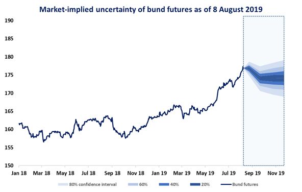
Analysing future uncertainty

A practical way to display future uncertainty is to create a fan chart with different option maturities
on the x-axis and different quantiles on the y-axis, separated with colour shading, which indicates
different levels of uncertainty. Fan charts help visualise probabilities associated with future outcomes,
and the balance of risks to the futures price.

Figure 17: Historical Bund futures prices and their forecasted option-implied quantiles for August,
September and October 2019 option maturities as of 8 August 2019 (the downward shift in
expectations is caused by the roll in the underlying futures contract, from September to December
contract). Source: Bloomberg, authors’ calculations.

From the fan chart, we can observe that implied uncertainty increases with time to maturity and the
balance of risks is slightly skewed to the downside (market pricing shows lower Bund futures prices
are more likely than higher prices).

An option-implied distribution of futures prices at a particular date in the future, combined with a
thorough survey across a spectrum of market participants can offer additional insights into the balance
of risks at a future date and how materially the risks are being perceived. An option implied PDF can
be, for example, combined with a histogram constructed from market participants’ expectations. The
shape of the histogram and the implied distribution reveals to what extent the market is sensitive to
a particular event, such as a central bank policy surprise. This information cannot be extracted from
futures or forward markets only.

One word of caution regarding surveys is that in many surveys, market participants are asked to
express their expectations, i.e. their average forecast, and they do not forecast the distribution of

 28