Search for Yield in Housing Markets. y - Carlos Garrigaz, Pedro Getex, Athena Tsouderou December 2020 - American Economic ...
←
→
Page content transcription
If your browser does not render page correctly, please read the page content below
y
                Search for Yield in Housing Markets.

                     Carlos Garrigaz, Pedro Getex, Athena Tsouderou{

                                           December 2020

                                                Abstract

          We study how investors in housing markets have changed after the 2009 …nancial
      crisis and the consequences for the markets and the economy. We document several new
      facts: (a) Institutional investors have replaced individual investors, but small size investors
      dominate among these new investors. (b) Most new investors are buy-and-hold investors
      as they are less likely to sell the properties in the short-term in response to capital gains.
      (c) Their investment portfolio has a strong local bias and is driven by search for yield. The
      arrival of buy-and-hold institutional investors has substantially lowered price momentum
      in housing markets.

          Keywords: Investors, Housing Prices, Rental Yield, Homeownership, Residential In-
      vestment, Housing, Flipping, Price Momentum.

     We thank Itzhak Ben-David, Morris Davis, Anthony DeFusco, Adam Guren, Jonathan Halket, Finn Kyd-
land, Charles Nathanson, Rafael Repullo, Vahid Saadi, Martin Schneider, and seminar participants at ESADE,
IESE, 2019 SED Conference and 2020 HULM Meeting at NYU.
   y
     The views expressed herein do not necessarily re‡ect those of the Federal Reserve Bank of St. Louis or
the Federal Reserve System. Research Reported in this paper was partially funded by the Spanish Ministry
of Economy and Competitiveness (MCIU), State Research Agency (AEI) and European Regional Development
Fund (ERDF) Grant No. PGC2018-101745-A-I00.
   z
     Federal Reserve Bank of St. Louis. carlos.garriga@stls.frb.org.
   x
     IE Business School, IE University. pedro.gete@ie.edu.
   {
     IE Business School, IE University. athenatsouderou@gmail.com.

                                                    1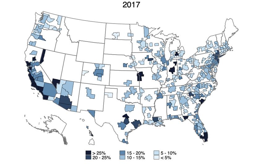
1       Introduction

     It is by now well-documented that during the housing boom of the 2000s investors in hous-
ing markets were typically private households who purchased multiple properties speculating
on housing price growth. These pre-crisis investors, also called “speculators”, purchased prop-
erty investments with a short-term horizon searching for capital gains. That is, these investors
bought and then sold as prices increased within one to two years (Bayer, Mangum, and Roberts
2016; Chinco and Mayer 2015; Gao, Sockin, and Xiong 2020; Haughwout, Lee, Tracy and Van
Der Klaauw 2011). The investment strategy of these investors generated persistent housing
price momentum (DeFusco, Nathanson, and Zwick 2020; Glaeser and Nathanson 2017; Guren
2018; Piazzesi and Schneider 2009).1

    In this paper we show that, post-crisis, the type of dominant investor has dramatically
changed. The investors after the crisis are not individuals but incorporated in the form of legal
entities. The vast majority of them are relatively small and local. They invest with a longer
term horizon in search for yield. The new investors react less to capital gains: they are 12
percent less likely to sell a house within two years, when capital gains increase by one standard
deviation from the mean. The new “buy-and-hold” investors have lowered price momentum
and the houses’time on the market. Consistent with these …ndings that investors post-crisis are
searching for yield, Daniel, Garlappi, and Xiao (2018) …nd that a low-interest-rate monetary
policy increases investors’demand for high-dividend stocks, which is more pronounced among
investors who fund consumption using dividend income. As rents are mostly stable, housing
becomes an investment asset and a close substitute to safe yield-earning investments (see for
example, Eisfeldt and Demers 2018).

    Our analysis is based on a large database containing all U.S. deeds.2 We show that small
investors, that is, those in the bottom 25th percentile in terms of dollar purchases, had the
largest growth post-crisis. The very large institutional investors, which have earned critical
attention in the media, invest only in speci…c locations.3

   The arrival of buy-and-hold investors to housing markets has a key real e¤ect that we test
and con…rm in the data. Since these investors react less to past housing price increases, then
housing price momentum should slow down. In other words, investors do not chase past capital
    1
      Housing price momentum refers to the price growth autocorrelation. Persistent, high, positive momentum
is often linked to behavioral biases.
    2
      Data provided by Zillow through the Zillow Transaction and Assessment Dataset (ZTRAX). More informa-
tion on accessing the data can be found at http://www.zillow.com/ztrax. The results and opinions are those of
the author(s) and do not re‡ect the position of Zillow Group.
    3
      For example, ninety percent of purchases by the top 20 “Wall Street Landlords” and the public apartment
REITs in 2015 are concentrated in 37 MSAs, which is less than 10 percent of all MSAs.

                                                     2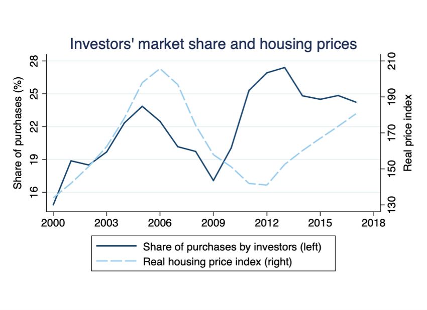
gains and thus avoid momentum purchases. DeFusco, Nathanson, and Zwick (2020) show that
the transaction volume leads to price growth, especially during housing bubbles. The arrival
of buy-and-hold investors did not increase as much the transaction volume, as it would have if
the investors were speculators. This is because buy-and-hold investors hold houses for a longer
time period before they resell. Lower transaction volume leads to less acceleration in prices.
As a consequence, housing price increases are less serially correlated in the short-term.

    This paper expands the established literature that studied investors in the previous housing
boom. This literature highlights that investors were individuals searching for capital gains. For
example, Garcia (2019) …nds that counties with higher share of investor activity experienced
higher house ‡ipping rates over 2005-2006, and higher increase in ‡ip rates between 2001 and
2005-2006. Bayer et al. (2016) show that speculation during the boom period was driven
by short-horizon investors as a response to past housing price increases. Haughwout et al.
(2011) document a large growth in ‡ippers in the early 2000s, and suggest that the relaxation
of borrowing constraints from increased housing prices led more optimistic buyers to enter
housing markets as short-term speculators. Gao, Sockin, and Xiong (2020) provide evidence
linking housing speculation during the previous housing boom to extrapolation by speculators
of past housing price changes. Other important papers studying the investors of the 2000s are
Chinco and Mayer (2015), DeFusco, Nathanson, and Zwick (2020), Albanesi, DeGiorgi, and
Nosal (2017), and Albanesi (2018). Our paper shows that the new investors post-crisis are
remarkably di¤erent from the speculators of the previous housing boom.

    Our second set of results relate to the literature on housing price momentum. This literature
shows strong evidence that prices in U.S. areas display signi…cant momentum (Glaeser and
Nathanson 2017; Guren 2018). The momentum lasts for up to 2-3 years before prices mean-
revert, a time horizon far greater than most other asset markets (Guren 2018). Glaeser and
Nathanson (2017) explain momentum based on behavioral biases of speculators in housing
markets. Based on this theory, investors underreact to news because of behavioral biases
or loss aversion and then “chase returns” because of extrapolative expectations about price
appreciation. Investors neglect to account for the fact that previous buyers were learning from
prices and instead take past prices as direct measures of demand. Piazzesi and Schneider
(2009) show evidence on trading based on the increased belief in rising housing prices, during
the housing boom of the 2000s. Our paper shows that the arrival of buy-and-hold investors
signi…cantly reduces housing price momentum.

    Our paper contributes to the literature studying the implications of the type of ownership
of the housing stock. Some early work by Chambers, Garriga, and Schlagenhauf (2009) uses
microdata and a structural model to explore the e¤ects of investor purchases in the supply

                                               3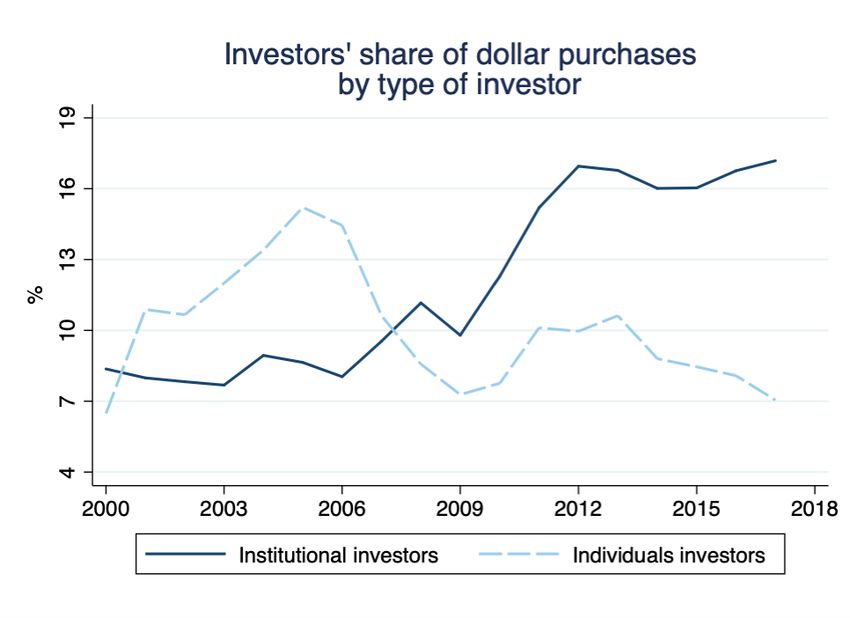
of rental housing, but in their analysis of the price of houses is determined by the cost of
constructing new units. More recently, Landvoigt, Piazzesi, and Schneider (2015) study the
di¤erent types of buyers during the housing boom of the 2000s in San Diego County, California,
but ignores the e¤ects in the rental market. The analysis in this paper integrates both views
and evaluates the e¤ects of who owns the housing stock in terms of prices and rents.

    Lastly, our paper touches on the recent literature that studies institutional investors in the
housing market. So far the literature has focused on documenting the increasing presence of
institutional investors in the single-family segment, in speci…c areas in the U.S. For example,
Allen et al. (2017) focusing on the Miami-Dade County in Florida, …nd that an increase in
the share of houses purchased by investors in a census block is related to an increase in house
prices. Raymond et al. (2018) …nd that large institutional owners of single-family rentals …le
more frequently eviction notices compared to small landlords in Fulton County in Atlanta.
Mills, Molloy, and Zarutskie (2019) show that prices increased in neighborhoods where large
buy-to-rent investors are concentrated. In a thorough analysis of institutional investors, using
deeds data from a di¤erent source, and conducting a zip code-level analysis in 20 large U.S.
MSAs, Lambie-Hanson, Li and Slonkosky (2019) …nd that single-family institutional buyers
contributed to an increase in price and rent growth, and a decline in homeownership rate change.
Their identi…cation is based on the First Look program, a program that gave households and
non-pro…ts an opportunity to bid on Fannie Mae and Freddie Mac’s real estate owned properties
before they became available to investors.4 Gallin and Verbrugge (2019) …nd that multi-unit
landlords, when renegotiating rent contracts, set rent increases that exceed the in‡ation rate,
aided by the law of large numbers and exploiting tenant moving costs.

   A more established literature has studied foreign and out-of-town investment in the housing
markets. See for example recent papers by Cvijanovic and Spaenjers (2020), Davids and Georg
(2020), and Favilukis and Van Nieuwerburgh (2018).

   The rest of the paper is organized as follows: Section 2 describes the data. Section 3 shows
the distributional results. Section 4 analyses the investment strategies pre- and post-crisis.
Section 5 presents the implications of searching-for-yield investments in housing. Section 6
concludes. The online appendix has extra information about the variables and results.
  4
      The …ndings are also included in a nontechnical report (Lambie-Hanson, Li, and Slonkosky 2018).

                                                       4
2 Data
The source of our data on investors in the U.S. housing market is the Zillow (2017) Transac-
tion and Assessment Dataset (ZTRAX). This database contains all property ownership transfers
in the U.S., as recorded by the counties’deeds. Our …nal sample contains all ownership trans-
fers of residential properties, including multi-family and single-family, from January 1st, 2000
to December 31st, 2017. These are 85 million transactions nationally.
We use a rigorous methodology to identify investors. First we distinguish between individ-
ual and non individual buyers based on the buyer name. Second, we …lter-out buyers that are
relocation companies, non pro…t organizations, construction companies and national and re-
gional authorities, as well as banks, Ginnie Mae, Fannie Mae, Freddie Mac and other mortgage
loan companies and credit unions, and the state taking ownership of foreclosed properties.
The housing variables come from Zillow. Housing prices come from the Zillow Home Value
Index for all homes, single-family homes, top tier homes and bottom tier homes at the County
and MSA levels. Top tier homes are homes in the top third, and bottom tier homes are homes
in the bottom third of the home value distribution within an MSA. The Zillow Home Value
Index is a dollar-denominated, smoothed, seasonally adjusted measure of the median estimated
home value across a given region and housing type. It is constructed using estimated monthly
sale prices not just for the homes that sold, but for all homes even if they didn’t sell in that
time period, which addresses the bias created by the changing group of properties that sell in
di¤erent periods of time. Housing rents come from the Zillow Rent Index for all homes, which
is constructed using a similar methodology to the Zillow Home Value Index.
We …nally collect county-year and MSA-year level controls, which are population from the
U.S. Census Bureau, unemployment rate from the U.S. Bureau of Labor Statistics, per capita
income from the Bureau of Economic Analysis, and median household income from Zillow.
More detailed description of the data sources is included in the online Appendix A.
Our …rst dataset contains transaction-level data, where the buyer is either an institutional
or an individual investor. This dataset contains all investors’purchases in 2003, 2004, 2013 and
2014, the duration until the next sale of the property and the capital gains and rental yields
at the time of sale, based on monthly median prices and quarterly median rents in the county
of the property. In total, this dataset consists of 2,068,562 observations. Table 1, Panel A
contains summary statistics of the key variables in our property-level analysis.
Our second dataset contains the market share of investors’ purchases at the MSA-level,
over the years 2009 to 2017. It also contains the average housing variables, control variables
5beginning in 2000, and tax-returns for the year 2007. In total this dataset consists of 332 MSAs.
Table 1, Panel B contains summary statistics of the key variables in our MSA-level analysis.
3 Distributional Results
In this section we de…ne investors in the housing market and present remarkable changes
in the distribution of investors, from pre- to post-crisis. Using very detailed micro-data at the
home purchase level, as described in the previous section, we use economic theory to break
down investors in di¤erent categories.
First, we distinguish in our data among institutional investors and individual investors. We
de…ne institutional investors as legal entities who purchase homes, that is, they use the name of
an LLC, LP, Trust, REIT, etc. in the purchase deed. We de…ne individual investors the buyers
who are individuals or households who purchase two or more properties within the same MSA
over a two-year period. Individuals who purchase multiple homes are likely to purchase them
as an investment, and not for them to live in. Our restriction in the classi…cation of individual
investors that they have to purchase within the same MSA, excludes individuals who purchase
their main residence and a holiday home in a di¤erent MSA. The remaining purchases in our
deeds are the homeowners, after excluding purchases by intermediaries.
To calculate the market share of investors we use the dollar value of purchases by investors
instead of the number of purchases since the number of purchases would underestimate presence
in the apartments market. For example the number of purchases would equate a purchase of one
condominium to the purchase of one apartment building of 100 apartments. The dollar value of
purchases re‡ects more accurately the presence of individuals and institutional investors in the
single-family and multi-family markets. Our variable of investors’presence is the share of the
dollar value of purchases by investors over the dollar value of all purchases, that is, by investors
and households. The total local market value accounts for economic shocks in each location
that a¤ect residential purchases.
The top panel of Figure 1 shows that the U.S. housing market experienced a surge in the
market share of purchases by total investors in the years following the 2008 …nancial crisis. It
shows the previous boom in investors’share of purchases and housing prices in the early 2000s,
and the collapse of both investors and prices after 2005-2006. From 2010 investors’ presence
in the housing market experiences a steep growth, while the housing prices begin to recover
after 2012. The bottom panel of Figure 1 shows a novel fact: institutional investors replace
and surpass the individual investors who experienced a boom in the years leading to the crisis.
6The largest share of purchases after the …nancial crisis is attributed to institutions.
Second, within the institutional investors, we examine the investors’ size, an important
parameter related to their real e¤ects. We calculate the size of institutional investors to be the
real dollar value of their purchases in each year. The top panel of Figure 2 plots the change
in the distribution of the institutional investors’ size in 2006 and 2015, to capture the pre-
and post-crisis periods.5 This …gure shows that mainly the small investors below the 35th
percentile of the size distribution, and, to a lesser extend, the very large investors, above the
95th percentile, had the largest growth in their purchases, from 2006 to 2015. The bottom panel
of Figure 2 shows that the increase in the small investors happened in the extensive margin
as well. The number of investors, and not only the aggregate dollar value of their purchases,
increased the most in the same period.6
The investors in the top one percent put remarkably large amounts of money into the
housing market with their purchases. The top one percent consists of the so-called “Wall
Street landlords”, private-equity backed investors, such as Blackstone’s Invitation Homes and
American Homes 4 Rent. The top one percent also includes the Apartment REITs such as
Equity Residential and AvalonBay Communities that are part of the newly formed Real Estate
Sector of the S&P 500 index. Although the top one percent holds signi…cant value of the
housing market, their purchases are geographically concentrated. For example, ninety percent
of purchases by the top Wall Street Landlords and the public apartment REITs in 2015 is
concentrated in 37 MSAs, which is less than 10 percent of all MSAs. In contrast, small investors
hold market share in almost all MSAs and they are likely to in‡uence the local housing markets.
Third, we investigate deeper who are the institutional investors, by classifying them into
local, out-of-town domestic and foreign. We de…ne local investors as the ones who have their
mailing address in the same MSA as the property they purchase. Out-of-town domestic in-
vestors are the ones who have their mailing address in the U.S., but outside the MSA of the
property they purchase. Foreign investors are the ones who have a mailing address outside the
U.S. Figure 4 plots the market share of institutional investors’dollar purchases split into the
above categories. About 55% of the institutional investors’purchases after 2009 is attributed
to local investors. Local investors are more likely to be small investors, for example mom-and-
pop investors that purchase homes in the MSA where they also live - and have their mailing
address. In the contrary, out-of-town domestic investors include the large REITs, having their
headquarters and mailing address for example in New York, and purchasing single-family prop-
erties in Tampa. Out-of-town domestic investors account for about 35% of the institutional
5
The purchase prices are converted to 2006 real dollars using the monthly CPI index.
6
Figure A1 uses the buyer’s mailing address as a unique identi…er, instead of the buyer’s name.
7investors’purchases after 2009. The market share of foreign institutional investors seems to be
negligible. Our data might not capture the full extend of foreign investment, as foreign legal
entities might use a U.S. mailing address, in which case they would be classi…ed as domestic
investors. Moreover, foreign individuals would be classi…ed as homeowners if they only make
one purchase within two years. To reconcile the share of foreign buyers with the 6.7% share
that Favilukis and Van Nieuwerburgh (2018) report over April 2015 to March 2016 in the U.S.,
and 10% the year after, we would need to add up the above di¤erent categories in our clas-
si…cation. Nevertheless, our data point to evidence that foreign investors are very unlikely to
drive our results. Moreover, we perform separate analyses using only the market share of local
institutional investors.
Figure A2 plots the market share of individual investors’ dollar purchases split by the
investors’origin. About 70% of individual investors are local, and there is minimal variation to
this percentage over the years. Figure A3 plots the market share of investors’purchases split
by the investors’origin, out of the total market.
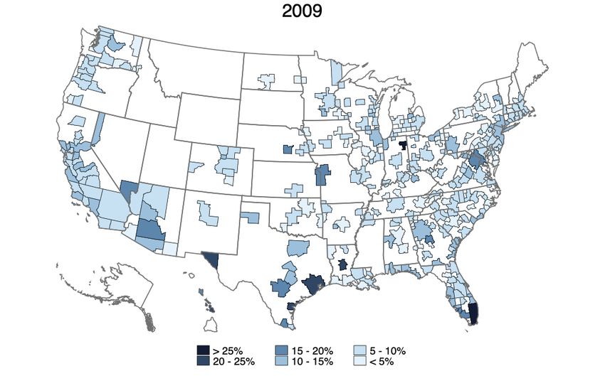
Lastly, Figure A4 illustrates that institutional investors have increased in most MSAs, with
large cross-sectional variations in their market share.
4 Search for Yield
The striking …ndings of the change in composition of investors, bring up the following
questions: How are the investors post-crisis di¤erent from the investors pre-crisis? How does
their investment strategy di¤er? Are they driven by search for capital gains or by search for
yields? Are the institutional investors contributing to creating a housing bubble in the same
way the individual investors contributed to the previous bubble? In this section we aim to
answer these questions.
The pre-crisis “speculators”primarily have been reselling houses in a short period, without
living in or renting them. Their motivation for the investment is capital gains (Haughwout et
al. 2011). In contrast, a buy-and-hold strategy would be less reactive to capital gains, and
would hold properties longer in search for rental yields.
To study the investment strategy of the pre-crisis investors, we focus on all the housing
purchases by investors in the U.S. from the beginning of 2003 until the end of 2004, which
we track until their next sale. Importantly, we track which of the houses purchased were sold
within two years of their purchase, that is before the end of 2006. This way we cover most of
8the housing boom period of the early 2000s. To study the investment strategy of the post-crisis
investors, we focus on all the housing purchases by investors in the U.S. from the beginning
of 2013 until the end of 2014, which we track until the end of our dataset on December 2017.
Equivalently to the pre-crisis period, we are interested whether these houses were sold within
two years of purchase, that is, up to the end of 2016, covering most of the post-crisis housing
boom. As we showed earlier, the periods 2003-2004 and 2013-2014 experienced high growth in
purchases by investors, although di¤erent types of investors.7
Our analysis consists of two steps. First, we estimate the sale price of all properties using
hedonic regression, and the implied capital gains from a short-term sale. Second, we estimate
how the capital gains are related to the probability of a short-term sale.
4.1 Hedonic estimation
In the …rst step, we use the following speci…cation to estimate the housing prices at the
time of purchase and at the time of sale:
log Pj = 0 + 1 Sizej + 2 Agej + 3 Renovj + z z Zipz + uj ; (1)
where j indexes the property. P j is the price of property j. Sizej is the size of the property,
measured in log square feet. Agej is the number of years from the time the property was built,
and Renovj is the number of years since the last renovation. Zipz are dummy variables that
take the value of one if the property is located in zipcode z.
We estimate (1) for the properties in our sample that were sold within two years of their
purchase, for which we have the purchase and the sale price. We estimate (1) separately for
each year of purchase 2003, 2004, 2013 and 2014. Table 2 contains the results of the hedonic
regressions.
We obtain sale price for all properties - not only the once sold within two years - as the linear
projection of the estimated coe¢ cients. Similarly we obtain the purchase price for all properties
purchased by investors from the hedonic estimations. We then calculate the short-term capital
gains as the percentage increase from the estimated purchase price to the estimated sales price.
That is, Gj = (Pjsell Pjpurchase )=Pjpurchase ; where Pjsell is the sales price and Pjpurchase is the
7
We do lots of sensitivity tests and …nd that the results are robust to the selection of pre- and post-crisis
boom years. Pre-crisis we are restricted to study housing purchases after the recession of 2001, and up to 2004,
so we can track the sales up to the end of the housing boom in 2006. Post-crisis we are restricted to study
housing purchases from the beginning of the housing boom in 2012, and up to 2015, so we can track the sales
up to the end of our dataset in 2017.
9purchase price of the property.
4.2 Buy-and-hold
In the second step, our analysis asks whether the investors post-crisis are more likely or less
likely compared to the pre-crisis investors to hold the property longer, based on their potential
capital gains. To study the probability of selling short-term, we estimate the following logit
model:
l(Sell)i;j = 0 + 1 Ii + 2 Gj + 3 Ii Gj + Cc + ui;j ; (2)
where i indexes the investor (buyer name) and j the property. l(Sell)i;j = log( 1 i;ji;j ); where i;j
is the probability of the property j that was bought by investor i to be sold within 2 years. Ii is a
binary variable that takes the value of one for investors post-crisis (who bought in 2013 or 2014)
and the value of zero for investors pre-crisis (who bought in 2003 or 2004). Gj is the capital
gains that would be realized if the property was sold within 2 years, estimated in the previous
step. While the capital gains were calculated separately for each year, to allow for di¤erent
economic conditions, we also include additional controls for housing demand. The controls Cc
include the growth in population, growth in per capita income, and change in unemployment
rate for each county, for the year of the property purchase and the following year.
We estimate the logit model (2) for the sample of all purchases by investors in the pre-crisis
years 2003-2004, and the post-crisis years 2013-2014. The estimation allows for robust standard
errors.
Next, we study the investment strategy of di¤erent types of investors post-crisis. To achieve
this we add in (2) interactions of the capital gains with dummies for di¤erent types of investors,
as follows:
l(Sell)i;j = 0 + 1 Gj + 2 Di + 3 Gj Di + Cc + ui;j ; (3)
where Di is a dummy for the largest institutional investors, or a dummy for out-of-town
and another dummy for foreign investors. We estimate the logit model (3) for the sample of
purchases by investors in the post-crisis years 2013-2014.
Table 3 shows the results of the estimation of (2). The coe¢ cient 3 is -0.23 percent, and
signi…cant at the 1% level. This means that in the presence capital gains the post-crisis investors
are less likely to sell the property in the short-term compared to pre-crisis investors. Keeping
all other things constant, investors post-crisis ‡ip their properties with 12.2% less probability
10based on one standard deviation increase in capital gains from the mean, compared to investors
pre-crisis.8
Figure 5 interprets the results of the interaction of pre- and post-crisis investors with the
capital gains. Figure 6 illustrates the previous results speci…cally for institutional and individual
investors. Table A1 shows that the results are robust if we use the time to sell as 1 year or 18
months.
Table 4 shows that the top investors, which are the 20 largest institutions in the market
of single-family rentals, were signi…cantly less likely to sell the properties in the short-term,
while they were more sensitive to capital gains, compared to the rest of the investors. Figure 7
interprets the estimated coe¢ cients.
Compared to the local investors, out-of-town buyers did not di¤er signi…cantly in their
short-term selling behavior. Foreign investors were signi…cantly less likely than the locals to
sell the properties within two years, but their sensitivity to capital gains was not signi…cantly
di¤erent.
5 Implications for Momentum
Housing price momentum means the positive time series autocorrelation of log price changes.
The literature shows considerable evidence that prices in U.S. areas display signi…cant momen-
tum (Glaeser and Nathanson 2017; Guren 2018; Ben-David 2011). The momentum lasts for up
to 2-3 years before prices mean-revert, a time horizon far greater than most other asset markets
(Guren 2018).
Glaeser and Nathanson (2017) provide a theory to explain momentum based on behavioral
biases of investors in the housing market. Based on this theory, investors underreact to news
because of behavioral biases or loss aversion and then “chase returns”because of extrapolative
expectations about price appreciation. Investors neglect to account for the fact that previous
buyers were learning from prices and instead take past prices as direct measures of demand.
Piazzesi and Schneider (2009) show evidence on trading based on the increased belief in rising
housing prices, during the housing boom of the 2000s.
We estimate the relationship between the market share of purchases by institutional investors
P
8 exp( P i xi )
To interpret the coe¢ cients of the logistic regression, we calculate the probability = 1+exp( i xi )
. An
increase in capital gains from the mean 32.86% to the mean plus one standard deviation (95.59%, from Table
1, Panel A) decreases the sale probability from 48.0% to 42.1%, which is a percentage decrease of 12.2%.
11and the price momentum during the recovery period 2009-2017. For comparison, we also
estimate the relationship between the market share of purchases by individual investors and
the price momentum during the previous housing boom of 2000-2005. Our speci…cation is as
follows:
Mm;09 17 = 0 + 1 Instm;09 17 + Cm;07 + s + um (4)
Similarly, the speci…cation for the study of the previous housing boom is:
0 0 0
Mm;00 05 = 0 + 1 Indm;00 05 + Cm;98 + s + um (5)
We de…ne the annual change in log housing price as Pm;t = Pm;t Pm;t 4 , where Pm;t is
the log real housing price in MSA m in quarter t. The autocorrelations Cor( Pm;t ; Pm;t+k )
summarize the serial correlation of log price changes over time and have been the focus in
the literature on the predictability of house prices, starting with Case and Shiller (1989) and
appearing in the most recent literature of momentum (e.g. Glaeser and Nathanson 2017;
Glaeser et al. 2014; Guren 2018; Head et al. 2014). We measure one-year price momentum
in MSA m for the years 2009-2017 as the 4-quarter lag serial autocorrelation of price changes
Mm;09 17 =Cor( Pm;t ; Pm;t+4 ), where t ranges from …rst quarter of 2009 to fourth quarter of
2016 in (4), and …rst quarter 2000 to fourth quarter 2004 in (5) : Having a smaller time period
pre-crisis to measure the momentum, gives a smaller average momentum than post-crisis.9 Our
focus however is in the direction of the correlation between share of investors and momentum.
Instm;09 17 is the average share of institutional investors’purchases over the total market
value of housing purchases in MSA m in the years 2009-2017. We also show the results for the
share of local institutional investors’purchases over the total market. Indm;00 05 is the average
share of individual investors’ purchases over the total market value of housing purchases in
MSA m in the years 2000-2005. Cm summarizes the MSA-speci…c controls, which are the log
population, log income and log price in 2007 in (4), and 1999 in (5). The speci…cations control
for state dummies s .
The results of the estimation of (4) and (5) are in Table 5. Individual investors increase
price momentum in line with the theory of behavioral biases and search for capital gains.
Interestingly institutional investors have the opposite e¤ect on momentum in the post-crisis
period. One percentage point increase in the average market share of institutional investors’
9
Our calculation of momentum for the years 1980-2011 gives an average of 0.61, for the largest 115 MSAs
that have price data in Zillow since 1980. This is very close to the average momentum Glaeser and Nathanson
(2017) report, using the same time frame and number of MSAs, and data from the Federal Housing Finance
Agency house price indices.
12purchases is related to 0.006 lower one-year price autocorrelation. For the local institutional
investors, the results are stronger. One percentage point increase in the average share of
local institutional investors’purchases is related to 0.011 lower one-year price autocorrelation.
This negative relationship between institutional investors and price momentum points to the
direction of our previous …ndings that the new institutional investors are less reactive to capital
gains than the traditional individual investors.
6 Conclusions
There has been a great amount of research on the characteristics of housing investors during
the previous housing boom. A consensus in the literature is that the housing investors in the
previous boom where speculators, they naively extrapolated expected price growth based on
previous-period price growth, and increased housing price momentum.
This paper undertakes a thorough data exercise to classify all house buyers in the U.S.
MSAs, for the period 2000 to 2017, into three mutually exclusive categories: institutional
investors, individual investors or homeowners. It further classi…es the properties purchased
by institutional investors into three mutually exclusive categories: houses purchased by local
investors, by out-of-town investors or by foreign investors. Focusing on institutional investors,
it divides them into percentile segments based on their size (dollar value of total purchases),
and singles out the large private equity …rms that entered the buy-to-rent market and publicly
traded apartment REITs. This is one of the …rst studies to provide detailed stylized facts
about the housing market investors in the U.S. and compare the investors before and after the
…nancial crisis.
By implementing hedonic regressions and estimating logit models, this paper shows evidence
that the new investors post-…nancial crisis are less reactive to capital gains, and hold the houses
longer to extract rental yields. Their longer investment horizon is related to lower housing
price momentum. These investment patterns are in line with a buy-and-hold strategy. The
results are also consistent with the recent literature in housing economics that shows di¤erential
patterns in the housing markets between the previous housing boom and the period post-crisis
in many advanced economies. Moreover, this study …nds that small local investors increased
their presence the most and drove most of these e¤ects. However, the investors who held the
houses the longest post-crisis were the large institutions that speci…cally entered the single-
family rental market to extract rental yields.
Important avenues for future research are to understand the drivers and motivations of
13the small local institutional investors. Monetary policy may have played a key role through a
portfolio rebalance channel. That is, the …ndings are consistent with the hypothesis that lower
returns on risk-free assets due to the implementation of large asset purchases during the crisis,
may have pushed investors to rebalance their portfolio by increasing exposure to alternative
assets such as real estate. More research is required to show this channel.
14References
Albanesi, S.: 2018, Real Estate Investors and the 2007-2009 Crisis. (Working Paper). Retrieved
from https://www.riksbank.se/globalassets/media/forskning/seminarier/2018/housing-
credit-and-heterogeneity-13-14-sept/albanesi— real-estate-investors-and-the-2007-2009-
crisis.pdf.
Albanesi, S., De Giorgi, G. and Nosal, J.: 2017, Credit growth and the …nancial crisis: A new
narrative. (NBER Working Paper No. 23740). Available at National Bureau of Economic
Research: https://www.nber.org/papers/w23740.
Allen, M. T., Rutherford, J., Rutherford, R. and Yavas, A.: 2018, Impact of investors in
distressed housing markets, The Journal of Real Estate Finance and Economics 56(4), 622–
652.
Bayer, P., Mangum, K. and Roberts, J. W.: 2016, Speculative fever: Investor contagion in
the housing bubble. (NBER Working Paper No. 22065). Available at National Bureau of
Economic Research: https://www.nber.org/papers/w22065.
Ben-David, I.: 2011, Financial constraints and in‡ated home prices during the real estate boom,
American Economic Journal: Applied Economics 3(3), 55–87.
Bernstein, A., Gustafson, M. T. and Lewis, R.: 2019, Disaster on the horizon: The price e¤ect
of sea level rise, Journal of Financial Economics 134(2), 253–272.
Case, K. E. and Shiller, R. J.: 1989, The e¢ ciency of the market for single-family homes,
American Economic Review 79, 125–137.
Chambers, M., Garriga, C. and Schlagenhauf, D. E.: 2009, Housing policy and the progressivity
of income taxation, Journal of Monetary Economics 56(8), 1116–1134.
Chinco, A. and Mayer, C.: 2015, Misinformed speculators and mispricing in the housing market,
The Review of Financial Studies 29(2), 486–522.
Cvijanovic, D. and Spaenjers, C.: 2018, ’We’ll always have Paris’: Out-of-country buy-
ers in the housing market. (SSRN Working Paper No. 3248902). Available at SSRN:
https://ssrn.com/abstract=3248902.
Daniel, K., Garlappi, L. and Xiao, K.: 2018, Monetary policy and reaching for income.
(NBER Working Paper No. 25344). Available at National Bureau of Economic Research:
https://www.nber.org/papers/w25344.
15Davids, A. and Georg, C. P.: 2020, The Cape of Good Homes: Exchange rate depreciations,
foreign demand and house prices. (SSRN Working Paper No. 3349815). Available at SSRN:
https://ssrn.com/abstract=3349815.
DeFusco, A. A., Nathanson, C. G. and Zwick, E.: 2020, Speculative dynamics of prices and
volume. (NBER Working Paper No. 23449). Available at National Bureau of Economic
Research: https://www.nber.org/papers/w23449.
Eisfeldt, A. and Demers, A.: 2018, Total returns to single family rentals. (NBER Working
Paper No. 21804). Available at https://www.nber.org/papers/w21804.
Favilukis, J. and Van Nieuwerburgh, S.: 2018, Out-of-town home buyers and city welfare. (SSRN
Working Paper No. 2922230). Available at SSRN: https://ssrn.com/abstract=2922230.
Gallin, J. and Verbrugge, R. J.: 2019, A theory of sticky rents: Search and bargaining with
incomplete information, Journal of Economic Theory 183, 478–519.
Gao, Z., Sockin, M. and Xiong, W.: 2020, Economic consequences of housing speculation, The
Review of Financial Studies . Forthcoming.
Garcia, D.: 2019, Second-home buying and the housing boom and bust, Finance and Economics
Discussion Series 19-029 . Board of Governors of the Federal Reserve System, Washington,
DC. Available at https://doi.org/10.17016/FEDS.2019.029r1.
Glaeser, E. L., Gyourko, J., Morales, E. and Nathanson, C. G.: 2014, Housing dynamics: An
urban approach, Journal of Urban Economics 81, 45–56.
Glaeser, E. L. and Nathanson, C. G.: 2017, An extrapolative model of house price dynamics,
Journal of Financial Economics 126(1), 147–170.
Guren, A. M.: 2018, House price momentum and strategic complementarity, Journal of Political
Economy 126(3), 1172–1218.
Haughwout, A., Lee, D., Tracy, J. S. and Van der Klaauw, W.: 2011, Real estate investors,
the leverage cycle, and the housing market crisis. (Sta¤ Report, No. 514). Federal Reserve
Bank of New York, NY. Available at: https://www.econstor.eu/handle/10419/60965.
Head, A., Lloyd-Ellis, H. and Sun, H.: 2014, Search, liquidity, and the dynamics of house prices
and construction, American Economic Review 104(4), 1172–1210.
Lambie-Hanson, L., Li, W. and Slonkosky, M.: 2018, Investing in Elm Street: What hap-
pens when …rms buy up houses?, Economic Insights pp. 9–14. Federal Reserve Bank of
16Philadelphia, PA. Retrieved from https://www.philadelphiafed.org/-/media/research-and-
data/publications/economic-insights/2018/q3/eiq318-elmstreet.pdf?la=en.
Lambie-Hanson, Lauren, W. L. and Slonkosky, M.: 2019, Leaving households behind:
Institutional investors and the U.S. housing recovery. (Working Paper 19-1). Fed-
eral Reserve Bank of Philadelphia, PA. Available at https://www.philadelphiafed.org/-
/media/research-and-data/publications/working-papers/2019/wp19-01.pdf.
Landvoigt, Tim, Monika Piazzesi, and Martin Schneider: 2015, The housing market(s) of San
Diego, American Economic Review 105(4), 1371–1407.
Mills, J., Molloy, R. and Zarutskie, R.: 2019, Large-scale buy-to-rent investors in the single-
family housing market: The emergence of a new asset class, Real Estate Economics
47(2), 399–430.
Piazzesi, M. and Schneider, M.: 2009, Momentum traders in the housing market: Survey
evidence and a search model, American Economic Review 99(2), 406–411.
Raymond, E. L., Duckworth, R., Miller, B., Lucas, M. and Pokharel, S.: 2016, Corporate
landlords, institutional investors, and displacement: Eviction rates in single-family rentals,
Community Economic Development Discussion Paper . Federal Reserve Bank of Atlanta,
GA.
Stroebel, J.: 2016, Asymmetric information about collateral values, The Journal of Finance
71(3), 1071–1112.
Zillow: 2017, ZTRAX: Zillow Transaction and Assessor Dataset, 2017-Q4. Zillow Group, Inc.
http://www.zillow.com/ztrax/.
17Figures
Figure 1. Presence of investors in the U.S. housing market. The top …gure plots the
average market share of investors’dollar purchases (left y-axis) and the national index of real
housing prices (right y-axis). The investors’data are annual MSA averages, for 411 U.S. MSAs
and MSA divisions, between 2000 and 2017. Investors refer to both institutional investors and
individuals. Institutional investors are classi…ed by their legal entity name. Individual investors
are those individuals who purchase more than one house within two years in the same MSA. The
bottom …gure plots the average market share of the investors’purchases, by type of investor.
The investors’share is weighted by the MSA market size. Appendix A describes the data.
18Figure 2. Size distribution of institutional investors. The …gure plots the dollar
purchases by institutional investors from 2006 to 2015 in each percentile segment of purchase
value. The percentile cuto¤s are the dollar values of the cuto¤s in 2006. All dollar values are
in 2006 dollars.
19Figure 3. Growth of institutional investors by size. The top …gure plots the growth
in dollar purchases by institutional investors from 2006 to 2015 in each percentile segment of
purchase value. The percentile cuto¤s are the dollar values of the cuto¤s in 2006. All dollar
values are in 2006 dollars. The bottom …gure shows the change in the number of investors
(extensive margin) over the same period.
20Figure 4. Local and out-of-town investors. The …gure plots the market share of insti-
tutional investors’dollar purchases split into local, out-of-town domestic and foreign investors.
We de…ne local investors as the ones who have their mailing address in the same MSA as the
property they purchase. Out-of-town domestic investors are the ones who have their mailing
address in the U.S., but outside the MSA of the property they purchase. Foreign investors
are the ones who have a mailing address outside the U.S. The investors’data are annual MSA
averages, for 411 U.S. MSAs and MSA divisions, between 2000 and 2017.
21Figure 5. Probability of sale in two years pre- and post-crisis. The …gure plots the
estimated probability of short-term sale (sale within two years from the month of purchase) for
the properties purchased by investors pre-crisis during 2003 and 2004, and post-crisis during
2013 and 2014. The vertical lines show the 90% con…dence intervals. The probabilities are
derived from the estimation of the logit model (2) described in section 4.2, and shown in Table
3.
22Figure 6. Probability of sale in two years pre- and post-crisis by type of investor.
The top …gure plots the estimated probability of short-term sale (sale within two years from the
month of purchase) by institutional investors for the properties purchased by investors pre- and
post-crisis. The bottom …gure plots the same estimated probabilities for individual investors.
The vertical lines show the 90% con…dence intervals. The probabilities are derived from the
estimation of the logit model (2) described in section 4.2.
23Figure 7. Probability of sale in two years post-crisis by investor size. The …gure
plots the estimated probability of short-term sale (sale within two years from the month of
purchase) for the properties purchased by investors post-crisis, for the largest institutional
investors in the single-family rental market, and the rest of the investors. The vertical lines
show the 90% con…dence intervals. The probabilities are derived from the estimation of the
logit model (3) described in section 4.2, and shown in Table 4.
24Tables
Table 1. Summary statistics
Panel A - Property and County level
Pre-crisis Post-crisis
Mean SD Min Max Mean SD Min Max
Sale in two years 0.30 0.46 0 1 0.30 0.46 0 1
Capital gain (%) 15.25 79.21 -170 253 32.86 95.59 -236 262
Avg. population growth (%) 1.74 1.92 -1.65 11.25 1.13 0.95 -7.13 12.17
Avg. income growth (%) 5.53 2.16 -2.89 20.11 4.16 1.59 -15.12 10.76
Avg. unempl. rate change (pp) -0.43 0.35 -1.7 0.95 -0.94 0.41 -2.35 1.55
Observations 1,115,296 953,266
Panel B - MSA level
Obs Mean SD Min Max
Institutional investors’market share (%) 332 12.45 7.79 3.10 41.26
Local institutional investors’market share (%) 332 6.48 6.05 0.00 37.03
Individual investors’market share (%) 332 5.83 3.20 0.66 27.82
Local individual investors’market share (%) 332 4.31 2.87 0.00 23.56
Individual investors’market share00 06 (%) 332 7.94 5.61 0.00 56.96
Momentum 332 0.48 0.30 -0.70 0.93
Momentum00 05 332 0.12 0.48 -0.92 0.91
Panel A presents summary statistics of the key variables at the property purchase level. The
sample consists of all residential property purchases by institutional and individual investors
in 2003-2004, and 2013-2014, which we track until their next sale. Capital gains are calculated
based on hedonic regression. Population growth, per capita income growth and unemployment
rate change are at the county level. Panel B presents summary statistics for the sample of all
MSAs with complete data. The variables are average annual values from 2009 to 2017, unless
denoted otherwise. Detailed description of the variables and data sources is in Appendix A:
25Table 2. Hedonic regression
Year 2003 2004 2013 2014
Log Price
Size 0.130*** 0.129*** 0.129*** 0.130***
(0.002) (0.002) (0.002) (0.002)
Age -0.225*** -0.236*** -0.203*** -0.202***
(0.017) (0.014) (0.016) (0.016)
Last renovation -0.407*** -0.396*** -0.494*** -0.514***
(0.018) (0.015) (0.016) (0.017)
Zipcode dummies Yes Yes Yes Yes
R-squared 0.617 0.630 0.700 0.703
Observations 135,940 181,639 135,348 125,017
Standard errors are in parentheses. The years indicate the year of the purchase of the
property. Size is the size of the property, measured in log square feet, age is the number of
years from the time the property was built, and last renovation is the number of years since the
last renovation. The coe¢ cients and standard errors for age and last renovation are multiplied
by 100. Each observation is a property. ***sig. at 1%.
26Table 3. Probability of short-term sale and investors
Short-term sale (sale in two years from purchase)
Capital gain 0.297*** 0.428*** 0.466***
(0.029) (0.031) (0.028)
Capital gain Post-crisis -0.232*** -0.248***
(0.038) (0.046)
Post-crisis 0.018 -0.074
(0.061) (0.052)
County-level controls No No Yes
Observations 2,068,562 2,068,562 2,041,615
Number of counties 924 924 895
Robust standard errors are in parentheses. The coe¢ cients and standard errors of capital
gains and the interaction are multiplied by 100. The county controls are the average growth
in population, growth in per capita income, and change in unemployment rate for two years
from the property purchase. Table A1 tests the robustness of the results to di¤erent durations.
***sig. at 1%.
27Table 4. Post-crisis: Probability of short-term sale and investors
Short-term sale (sale in two years from purchase)
Capital gain 0.210*** 0.208***
(0.034) (0.028)
Capital gain Top investors 0.765***
(0.130)
Top investors -3.069***
(0.133)
Capital gain Out-of-town buyer -0.108*
(0.060)
Out-of-town buyer -0.041
(0.088)
Capital gain Foreign buyer 0.098
(0.080)
Foreign buyer -1.200***
(0.089)
County-level controls Yes Yes
Observations 946,797 858,567
Number of counties 892 823
Robust standard errors are in parentheses. The coe¢ cients and standard errors of capital
gains and the interaction are multiplied by 100. The county controls are the average growth
in population, growth in per capita income, and change in unemployment rate for two years
from the property purchase. Table A1 tests the robustness of the results to di¤erent durations.
***sig. at 1%.
28Table 5. Housing price momentum and investors’share
Years 2000-2005 2009-2017
Price momentum
Investors’sharem;00 05 0.011**
(0.005)
Investors’sharem;09 17 -0.006**
(0.003)
Observations 321 320
Standard errors are in parentheses. Momentum is the one-year serial autocorrelation of
annual log real price changes, calculated from quarterly prices. Controls are the log population,
log income and log real price in 2007 in the …rst and second columns, and 1999 in the third
column. All models include state dummies. Each observation is an MSA. ***signi…cant at the
1% level; **signi…cant at the 5% level.
29ONLINE APPENDIX (Not for Publication)
A Detailed Description of Database
In this section we describe our data sources, how we cleaned the data, and the key variables
used in our analysis.
Investors’purchases
The investors’data come from the Zillow Transaction and Assessment Dataset (ZTRAX),
a large new raw database of U.S. deeds data. The transactions database of ZTRAX contains all
property ownership transfers that are documented in the County deeds. Each record contains
the date of the transfer, the address of the property, the type of the property, the sale price,
and the names of the buyer and seller. We keep transactions between January 1st , 2000 and
December 31st , 2017. We restrict the data to ownership transfers, dropping observations that
refer exclusively to mortgages or foreclosures.10 We drop transactions with deed type “Life
Estate”, since this is not an immediate transfer of ownership. We also drop transactions that
had “Cancellation” in the deed type. We restrict the data to residential property transfers
based on the ZTRAX property land use standard codes, which include both single-family and
multi-family properties. Table A2 contains the classi…cation of the property land use standard
codes in single-family and multi-family from ZTRAX. This amounts to 139 million transactions
nationally. We then drop transactions with purchase price missing or smaller than $10,000, a
common practice with deeds data (Bernstein, Gustafson and Lewis 2019; Stroebel 2016). This
leaves 85 million transactions.
With the previous cleaning criterion, most of the transactions are dropped in the non-
disclosure states. These states or counties do not require that the sale price is submitted to the
county o¢ ce. Speci…cally, all transactions are dropped in …ve non-disclosure states: Mississippi,
Missouri, Montana, Utah and Wyoming. We keep in our data seven non-disclosure states, with
a total of 28 MSAs, in which some of the transactions record sales price.11 Additional results,
10
The mortgage and foreclosure deeds have a separate corresponding deed for the ownership transfer.
11
The …nal dataset contains the following MSAs in non-disclosure states: Anchorage, Alaska; Boise City,
Idaho; Alexandria, Baton Rouge, Hammond, Houma-Thibodaux, Lafayette, Lake Charles, Monroe, New
Orleans-Metairie and Shreveport-Bossier City, Louisiana; Kansas City and Wichita, Kansas; Albuquerque, New
Mexico; Bismarck and Fargo, North Dakota; Amarillo, Austin-Round Rock, Brownsville-Harlingen, Corpus
Christi, Dallas-Plano-Irving, El Paso, Fort Worth-Arlington, Houston-The Woodlands-Sugar Land, Killeen-
Temple, Lubbock, McAllen-Edinburg-Mission and San Antonio-New Braunfels, Texas.
30not reported here, contain our cross-sectional analysis, dropping completely all non-disclosure
MSAs. The results hold with the same signi…cance and even stronger results for the relevance
tests for our instrumental variable.
To identify institutional investors, we …rst use the ZTRAX classi…cation of buyer names into
individual and non-individual names. The non-individual names frequently end with the words
“LLC”, “LP”, “INC”, “TRUST”, “CORPORATION”, “PARTNERS”, but they also contain
entity names without the description in the end of the name.12 Thorough inspection of the
data con…rms that the classi…cation by ZTRAX of individual and non-individual names is as
expected, with very minimal (human) errors. Our institutional investors’identi…er contains the
deeds where the buyer has a non-individual name. From these names we …lter out names of
relocation companies, non pro…t organizations, construction companies, national and regional
authorities, banks, Ginnie Mae, Fannie Mae, Freddie Mac and other mortgage loan companies
and credit unions, homeowner associations, hospitals, universities (not when is university hous-
ing), churches, airports, and the state, names of the county, city and municipality. To identify
relocation companies, non pro…t organizations and construction companies we use public data
of lists of the top relocation companies, non pro…t organizations and construction companies
in the U.S. We also manually check the names of the 200 largest non-individual buyers in
each state using online search engines to classify them in the right category, and iterate this
procedure several times to ensure the largest buyers are correctly classi…ed.
To further increase the accuracy of the largest institutional investors’classi…cation we collect
from industry reports and news reports the names of the top 20 institutional investors in the
single-family rental market. For example Amherst Capital’s 2018 market commentary report13
provides a comprehensive list of the top 20 single-family rental institutions and the number
of homes owned based on their calculations. We also collect the names of the residential real
estate companies that belong to the S&P 500 Real Estate Index, most of which are apartment
REITs. We then search for the names of these top investors and their subsidiaries in the
ZTRAX database and ensure they are classi…ed as institutional investors. We use public SEC
…lings and other business websites to track down the names of the subsidiaries of these large
investors. This procedure results in calculating the exact holdings of the top single-family and
multi-family institutional investors.
To classify non-institutional buyers into individual investors we start from the ZTRAX
classi…cation of buyer names as names of individuals. We calculate the number of purchases
12
For example "Invitation Homes" and "Invitation Homes LP" are both included as non-individual names.
13
Amherst Capital report is retrieved from https://www.amherstcapital.com/documents/20649/22737/
Amherst+Capital+Market+Commentary+-+April+2018+vF/f06bd51a-44c7-4f8f-87e3-
ca8d795bf42a Last visited: 03-05-2019.
31of each individual name within the MSA within the given year and the year before. We de…ne
individuals that are investors as individuals who purchase more than one property within the
MSA in the given year and the year before.
We calculate the market share of investors as the dollar value of investors’purchases (either
individual or institutional, or local institutional investors) divided by the dollar value of all
purchases, by institutional and individual investors and homeowners. Using the dollar value,
accounts correctly for purchases of buildings with multiple units.
We also code the number of units of each purchase. The number of units is coded initially
by ZTRAX, in the tax assessment dataset, which we merge with the transactions dataset, using
the RowID unique identi…er. We use the property type code (PropertyLandUseStndCode) to
…ll in the missing number of units. Speci…cally, we …ll in number of units 2 if number of units is
missing and the property type is duplex or multifamily dwelling (generic any combination 2+).
We …ll in number of units 3 for triplex, 4 for quadruplex, and 5 for apartment building (5+
units) or court apartment (5+ units). We …ll in number of units 100 for apartment building
(100+ units). With this criterion, when the number of units is missing we assign the lower
bound of the number of units to the property, inferred by the qualitative description. For the
rest of the multi-family property types and all the types we classify as single-family in Table
A2 that do not specify number of units, we assign 1 unit. We double-check with the sales price
and con…rm that these refer to single-unit purchases. For our analysis of single-unit purchases
we exclude from the sample all purchases of properties of two or more units.
The holding duration is the duration between the purchase and sale of the property. We
de…ne long-term investments the purchases that are held for more than one year, and short-term
investments the purchases that are sold within a year, to illustrate the descriptive statistics of
the ZTRAX data.
Finally, we use the crosswalk …le from Census Bureau to match the County FIPS codes
in ZTRAX to the Census Bureau MSA’s 2017 core based statistical area (CBSA) code. For
submetro areas of the largest MSAs, we use the CBSA division code. In total we match 411
CBSAs in the data. Tables A3 to A6 contain descriptive statistics of the ZTRAX data (before
merging with other variables).
Other variables
We also rely on the following data sources to get data at the county-year level and then
aggregate to MSA-year level using the 2017 CBSA and CBSA division codes:
32You can also read