High-Quality SNP Linkage Maps Improved QTL Mapping and Genome Assembly in Populus
←
→
Page content transcription
If your browser does not render page correctly, please read the page content below

Journal of Heredity, 2020, 515–530
                                                                                                               doi:10.1093/jhered/esaa039
                                                                                                                           Original Article
                                                                                            Advance Access publication September 15, 2020

Original Article

High-Quality SNP Linkage Maps Improved QTL
Mapping and Genome Assembly in Populus

                                                                                                                                                                Downloaded from https://academic.oup.com/jhered/article/111/6/515/5905935 by guest on 12 December 2020
Chunfa Tong, Dan Yao, Hainan Wu, Yuhua Chen, Wenguo Yang, and
Wei Zhao
From the Co-Innovation Center for Sustainable Forestry in Southern China, College of Forestry, Nanjing Forestry
University, Nanjing 210037, China.

Address correspondence to C. Tong at the address above, or e-mail: tongchf@njfu.edu.cn.
Received June 15, 2020; First decision July 28, 2020; Accepted September 11, 2020.

Corresponding Editor: Mark Chapman

Abstract
With the advances in high-throughput sequencing technologies and the development of new
software for extracting single nucleotide polymorphisms (SNPs) across a mapping population,
it is possible to construct high-quality genetic maps with thousands of SNPs in outbred forest
trees. Two parent-specific linkage maps were constructed with restriction site-associated DNA
sequencing data from an F1 hybrid population derived from Populus deltoides and Populus simonii,
and applied in QTL mapping and genome assembly. The female P. deltoides map contained 4018
SNPs, which were divided into 19 linkage groups under a wide range of LOD thresholds from 7 to
55. The male P. simonii map showed similar characteristics, consisting of 2097 SNPs, which also
belonged to 19 linkage groups under LOD thresholds of 7 to 29. The SNP order of each linkage
group was optimal among different ordering results from several available software. Moreover,
the linkage maps allowed the detection of 39 QTLs underlying tree height and 47 for diameter at
breast height. In addition, the linkage maps improved the anchoring of 689 contigs of P. simonii
to chromosomes. The 2 parental genetic maps of Populus are of high quality, especially in terms
of SNP data quality, the SNP order within linkage groups, and the perfect match between the
number of linkage groups and the karyotype of Populus, as well as the excellent performances in
QTL mapping and genome assembly. Both approaches for extracting and ordering SNPs could be
applied to other species for constructing high-quality genetic maps.

Subject areas: Quantitative genetics
Keywords: genetic linkage map, restriction site-associated DNA sequencing, single nucleotide polymorphism, quantitative trait
locus, genome assembly, Populus

The genus Populus comprises approximately 30 species of deciduous                         Tacamahaca, Turanga), although some controversies remain unre-
flowering trees in the willow family (Salicaceae) and is widely dis-                      solved (Eckenwalder 1996; Wang et al. 2014). Most of these species
tributed in the Northern Hemisphere (Boes and Strauss 1994).                              are of great commercial and ecological importance because they are
Three common names, poplar, aspen, and cottonwood, refer to dif-                          fast-growing trees and can provide valuable raw materials within a
ferent Populus species (Sannigrahi et al. 2010). According to mor-                        short period of time for the production of pulp and paper, wood-
phological similarity and crossability, the species within this genus                     based panels, biofuels, and other biobased products (Sannigrahi
are grouped into 6 sections (Abaso, Aigeiros, Leucoides, Populus,                         et al. 2010; Zhigunov et al. 2017). This genus has been chosen as a

© The American Genetic Association 2020.
                                                                                                                                                         515
This is an Open Access article distributed under the terms of the Creative Commons Attribution Non-Commercial License (http://creativecommons.org/
licenses/by-nc/4.0/), which permits non-commercial re-use, distribution, and reproduction in any medium, provided the original work is properly cited.
For commercial re-use, please contact journals.permissions@oup.com.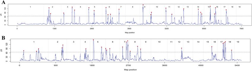
516                                                                                               Journal of Heredity, 2020, Vol. 111, No. 6

model system for forest trees due to biological characteristics such          To perform genetic linkage mapping and QTL analysis in Populus,
as a small genome size (~480 Mbp), a fast growth rate, and the ease       we established an F1 hybrid population by crossing P. deltoides and
of asexual and seed reproduction (Woolbright et al. 2008). Whole-         P. simoniii over 3 years from 2009 to 2011. The female parent,
genome sequences are now available for several species of the genus,      P. deltoides, and the male parent, P. simoniii, exhibit substantial dif-
including Populus trichocarpa (Tuskan et al. 2006), P. euphratica         ferences in their growth rates and stress responses, thus producing
(Ma et al. 2013), and P. deltoides (http://www.phytozome.net).            permanent material for genetic mapping (Mousavi et al. 2016). In
However, the completion of these valuable genome resources re-            our previous studies (Mousavi et al. 2016; Tong et al. 2016; Yao
lied on genetic linkage maps for resolving misassembly issues and         et al. 2020), different strategies for performing genetic mapping
anchoring chromosome-scale sequences (Fierst 2015). A genetic             with RADseq data from the F1 population were investigated, ultim-
linkage map that displays the linear orders and genetic distances of      ately leading to the development of the novel software gmRAD for
groups of molecular markers has been used for over 100 years, since       de novo extraction of high-quality SNP genotypes. In the present
the first linkage map was generated for Drosophila melanogaster           study, we incorporated more individuals from the F1 hybrid popula-
(Sturtevant 1913). Indeed, genetic linkage maps not only play an          tion to construct 2 parental high-quality genetic maps, and gmRAD

                                                                                                                                                     Downloaded from https://academic.oup.com/jhered/article/111/6/515/5905935 by guest on 12 December 2020
essential role in the assembly of genome scaffolds and comparative        was utilized for the generation of high-quality SNP genotypes solely
genomics (Krutovsky et al. 2004; Kakioka et al. 2013) but are also        from RADseq data. Additionally, a new strategy was adopted for
prerequisites for identifying quantitative trait loci (QTLs), which in-   obtaining the optimal order of SNPs within a linkage group, which
dicates the relationship between phenotype and genotype in plants         was highly beneficial to the quality of the 2 linkage maps. Based on
and animals (Lander and Botstein 1989; Zeng 1994).                        the newly constructed parental linkage maps, we further performed
    Although the precision and accuracy of a genetic map are af-          QTL analysis of tree height (H) and diameter at breast height (DBH)
fected by many factors, such as the population size, the number           with phenotypic data measured over 5 years. The candidate genes
of available genetic markers, and the methods used for ordering           of the detected QTLs and their relationship with QTLs previously
markers within a linkage group (Tao et al. 2018), considerable ef-        identified in other studies were also investigated. In addition, the
forts have been devoted to constructing genetic linkage maps in at        linkage maps significantly improved the anchoring of a draft genome
least 10 Populus species for the past 3 decades (Wang et al. 2011).       sequence of the male parent P. simonii to the chromosomes.
Most linkage maps generated in Populus are sparse due to the use
of a small population size (
Journal of Heredity, 2020, Vol. 111, No. 6 517
DNA Extraction and RAD Sequencing (Mousavi et al. 2016; Tong et al. 2016). We used these 2 SNP segre-
In the springs of 2013 and 2016, fresh leaf tissue was collected gation datasets to construct the linkage maps of female P. deltoides
from the 2 parents and a total of 418 progeny. The samples were and male P. simonii separately. First, each dataset was divided into
stored in a −80°C freezer, and DNA was extracted according to the linkage groups under an LOD threshold after performing 2-point
manufacturer’s protocol of the Plant Genomic DNA Kit (Tiangen, linkage analysis with the software FsLinkageMap (Tong et al. 2010).
Tiangen Biotech Co. Ltd., Beijing, China) or following the CTAB Second, the SNPs in each linkage group were ordered with different
protocol (Doyle and Doyle 1987). The RAD library for each indi- types of available software that can be used for genetic mapping
vidual was constructed basically following the protocol described in an F1 hybrid population of outbred species. We used JoinMap
by Baird et al. (Baird et al. 2008). Briefly, genomic DNA from each (Van Ooijen 2006), OneMap (Margarido et al. 2007), and Lep-MAP
sample was digested with the restriction enzyme EcoRI (NEB, USA), (Rastas et al. 2013) to order the SNPs within a linkage group 5, 1,
and a P1 adaptor containing a MID (molecular identifier) was then and 3 times, respectively. Among the ordering results from the 3 soft-
ligated to the products of the restriction reaction. Thereafter, the ware programs, we chose the optimal result for the final map based
DNA samples were pooled and randomly sheared by sonication be- on the ordering-objective function of the minimum sum of adjacent
Downloaded from https://academic.oup.com/jhered/article/111/6/515/5905935 by guest on 12 December 2020
fore the addition of the paired-end P2 adaptor. Libraries with an in- recombination fractions (SARF) (Falk 1989). Third, to match the
sert size ranging from 300 to 500 bp were prepared and sequenced linkage groups with chromosomes, we extracted a flanking sequence
from both ends (paired-end) with 82–150 bp read lengths. The RAD of 41 bp for each SNP and aligned it with BLAST to the reference
sequencing of all the individuals was performed at 5 different times genome of P. trichocarpa. Therefore, the linkage group number was
in 4 sequencing companies. In 2013, the 2 parents and 150 progeny determined to be the chromosome number if the majority of its SNPs
were sequenced in 8 lanes on the Illumina HiSeq 2000 platform at were mapped to the reference chromosome. Finally, linkage maps
Novogene Bioinformatics Institute, Beijing, China (NBI), while the were first plotted in WMF format with Kosambi’s genetic mapping
same 2 parents and another 150 progeny were sequenced in 7 lanes function (Kosambi 1944) by FsLinkageMap, and then further modi-
on the Illumina HiSeq 2000 platform at Beijing Genomics Institute, fied into PDF format with the software Mayura Draw (http://www.
Shenzhen, China (BGI) (Tong et al. 2016). In 2016, we also sequenced mayura.com).
39 progeny at Majorbio Company, Shanghai, China (MBC), 40 at
Genepioneer Biotechnologies, Nanjing, China (GPB), and 47 at BGI
on the Illumina HiSeq 4000 platforms. In addition to the 2 parents,
QTL Mapping for Longitudinal Growth Traits
there were 8 progeny that were each sequenced separately in 2 dif- We performed QTL analysis of the 2 growth traits (H and DBH) with
ferent sequencing companies (Supplementary Tables S1–S5). The same a phenotypic dataset obtained from the F1 hybrid population based
individual reads data from different companies can be used to validate on the parental linkage maps constructed in this study. The dataset
the accuracy of sequencing and subsequent SNP calling. included 5-year H and DBH data measured from 332 individuals
belonging to 109 clones. We applied the means of the growth traits
for each clone per year to conduct QTL analysis using the software
SNP Discovery and Genotyping
mvqtlcim (Liu et al. 2017), which is designed to implement composite
The raw data from each sequencing company were processed to
interval mapping (Zeng 1994) of longitudinal or multiple traits in an
generate so-called clear data via the following procedures: 1) each
outbred full-sib family. Because all the SNP markers in the linkage
sample reads were segregated by its unique nucleotide MID to gen-
maps segregate in a 1:1 ratio, the QTL segregation patterns were as-
erate the first and second read files in fastq format; 2) if the paired
sumed to be Qq×QQ in the maternal linkage map and QQ×Qq in
reads contained primer/adaptor sequences, they were removed from
the paternal linkage map. When performing the CIM calculations,
the fastq files; 3) if 10% of bases were uncalled in a single read, the
the number of background markers was iterated from 11 to 49 with
pair was deleted from the data files; and 4) if a single read contained
a step size of 2 and the window size was set to 10, 15, or 20 cM.
more than half low-quality bases (Phred score ≤5), the pair was also
For each parameter combination of the background marker number
removed from the dataset. To obtain high-quality (HQ) reads, the
(BMN) and window size (WS), the LR was calculated at each map
NGS QC toolkit (Patel and Jain 2012) was applied to further filter
position in steps of 1 cM, and the LR threshold for declaring a sig-
out those paired reads in which a single read contained more than
nificant QTL was determined from 1000 permutation tests (Doerge
30% bases that had a Phred score less than 20.
and Churchill 1996). To obtain the optimal mapping result, we fitted
We used the software gmRAD for SNP discovery and genotype
a multivariate linear regression model for each trait on the genotype
calling in the HQ read data for all individuals across the F1 map-
effects of all detected QTLs over the 5 time points for each parameter
ping population (Yao et al. 2020). The main parameters of the soft-
combination. The regression model can be expressed for N detected
ware used for analyzing the whole dataset were set as follows: 1) the
QTLs as follows:
hamming distance for grouping the first reads of each parent was
set to 5; 2) the edit distance for filtering mapped reads was set as N
5; 3) the coverage depth of an allele of a heterozygote was required yit = µt + (pij1 − pij2 )ajt + eit , i = 1, 2, · · · , n; t = 1, 2, · · · , 5
j=1
to be at least 3; 4) the percent of genome repeat regions was set to
~70% based on the genome sequence of P. trichocarpa (Tuskan et al. (1)
2006); 5) the minimum score of an SNP genotype was set as 30; where yit is the trait value of the ith clone at time t ; µt is the overall
6) the minimum percent of non-missing genotypes at an SNP was set mean at time t ; ajt is the homozygous genotype (QQ) effect of the jth
equal to 80%; and 7) the minimum P-value from the chi-squared test detected QTL at time t , while −ajt is the heterozygous genotype (Qq)
for the segregation ratio at an SNP was set as 0.05. effect; pij1 is the conditional probability of the jth QTL genotype QQ
on its flanking marker genotype and pij2 is the conditional probability
Genetic Map Construction for Qq (Liu et al. 2017); and eit is the random error at time t for the
Owing to the biological characteristics of the F1 hybrid population, ith individual. The coefficient of determination (R2) of model (1) for
the majority of SNPs segregated in the types of aa×ab and ab×aa each time point can be regarded as the proportion of the phenotypic518 Journal of Heredity, 2020, Vol. 111, No. 6
variance at that time explained by all detected QTLs. Therefore, the Results
optimal mapping result was chosen as the result that corresponded
RAD Sequencing Data
to the maximum mean R2 values over the time points among all the
parameter combinations. For the optimal mapping result, the effects A total of 1486.2 Gb RADseq data were obtained from the 2 parents
of each QTL over different times were re-estimated with model (1), and 418 progeny in the F1 hybrid population of P. deltoides and
and the corresponding heritabilities were calculated as the differences P. simonii. These data consisted of paired-end (PE) reads with dif-
in the R2 values when it was removed from the model. ferent lengths and came from the companies NBI, BGI, GPB, and
MBC, and were considered clean data because they were gently fil-
tered by the sequencing companies (as described in Materials and
Investigation of QTL Candidate Genes
Methods). All the clean data are available under accession numbers
To investigate the candidate genes for the identified QTLs, we first
in the NCBI SRA database (http://www.ncbi.nlm.nih.gov/Traces/
obtained the coding sequences (CDS) of those genes within the
sra), which were listed in Supplementary Tables S1–S5. After further
physical regions of QTLs from the gene annotation database of
filtering with the NGS QC toolkit (Patel and Jain 2012), we obtained
P. trichocarpa v3.1 at Phytozome (https://phytozome.jgi.doe.gov).
Downloaded from https://academic.oup.com/jhered/article/111/6/515/5905935 by guest on 12 December 2020
1385.0 Gb of high-quality (HQ) reads data for genetic mapping.
Then, the genes were re-annotated with Blast2GO by subjecting
Table 1 summarizes the clean and HQ data to provide the average
their CDSs to Blast searches against the protein database and then
information regarding reads number and base numbers for each of
mapping the hits to Gene Ontology (GO) terms. With the gene anno-
the 5 batches of sequencing conducted at the 4 companies. More
tations, we identified candidate genes for growth and development
details of each sample data are presented in Supplementary Tables
as well as response to stresses.
S1–S5, which includes the PE reads number, the number of bases,
the first and second read lengths, and the accession number prefixed
Chromosomal Assembly With Genetic Maps with SRR in the NCBI SRA database.
As a genome assembly application, we used the 2 parental linkage
maps constructed here to re-anchor the contigs of the male parent SNP Discovery and Quality Assessment
P. simonii to chromosomes. The draft genome assembly contained We analyzed the HQ reads with the software package gmRAD to
686 contigs with accession numbers from VJNQ02000001.1 to extract SNP genotype data for the 2 parents and 418 progeny in the
VJNQ02000686.1 at the NCBI, with a total length of 441.38 Mb F1 hybrid population. As expected, the majority of SNPs segregated
and a contig N50 of 1.94 Mb, which were assembled from single- in the types of aa×ab and ab×aa, which amounted to 2101 and 4021,
molecule long reads generated by the PacBio platform in our pre- respectively. We counted the number of non-missing genotypes at
vious study (Wu et al. 2020). First, the flanking sequence of each each of these SNPs and found that the average number was 388
SNP in the 2 linkage maps was subjected to Blast searches against (92.82%) and that the minimum number was 335. Additionally, we
the contigs by setting the query coverage value equal to 90%. For found that the missing genotype rate in an individual ranged from
an SNP, the best blast hit with a maximum query coverage and a 0.05% to 39.42% with an average value of 7.18%. To evaluate
minimum expected value was remained, letting it connect to a the accuracy of the genotypes at these SNPs, 8 progeny that were
unique contig. Next, 2 comma-delimited (csv) files for each parental sequenced independently at 2 different companies were used to con-
linkage map were prepared by recording the contig and the position firm the consistency of the genotypes. For each individual, the ratio
to which an SNP sequence was aligned as well as the linkage number of the number of SNP sites that were genotyped consistently with
and position of the SNP in the linkage map. Thereafter, we per- independent RADseq data was calculated. The consistency rate was
formed anchoring using the software ALLMAPS (Tang et al. 2015) shown to be very high, in the range of 98.61% to 99.98%, and the
with equal weights for the 2 linkage maps. overall rate was up to 99.59% (Supplementary Table S6).
Table 1. Summary of the average reads number of the RADSeq data with the number of bases in brackets for the 5 batches of sequencing
in the 4 companies
Batch Company Sample type Sample number Raw reads number (Gb) HQ reads number (Gb)
1 NBIa Male parent 1 14 024 713 (2.80) 12 617 155 (2.52)
Female parent 1 12 949 974 (2.59) 11 500 364 (2.30)
Progeny 150 4 555 004 (0.91) 4 084 337 (0.82)
2 BGIb Male parent 1 57 159 139 (9.91) 55 789 694 (9.68)
Female parent 1 21 619 787 (3.72) 20 956 868 (3.60)
Progeny 150 6 701 881 (1.16) 6 500 976 (1.13)
3 GPBc Progeny 40 9 880 332 (2.91) 9 869 660 (2.90)
4 MBCd Progeny 39 11 962 418 (3.68) 11 121 430 (3.29)
5 BGI Progeny 47 129 945 928 (19.08) 120 126 084 (17.63)
Total Male parent 1 71 183 852 (12.71) 68 406 849 (12.20)
Female parent 1 34 569 761 (6.31) 32 457 232 (5.90)
Progeny 418e 20 712 294 (3.51) 19 287 668 (3.27)
a
NBI: Novogene Bioinformatics Institute, Beijing, China.
b
BGI: Beijing Genomics Institute, Shenzhen, China.
c
GPB: Genepioneer Biotechnologies, Nanjing, China.
d
MBC: Majorbio Company, Shanghai, China.
e
In the progeny, there are 8 individuals each sequenced in 2 batches indipendently.Journal of Heredity, 2020, Vol. 111, No. 6 519
Genetic Linkage Maps with parameter values of BMN 49 and WS 10.0 for both parental
After performing 2-point linkage analysis with FsLinkageMap, 4018 linkage maps. Figure 5 shows the LR profiles of the 2 linkage maps,
SNPs segregating in ab×aa were grouped into 19 linkage groups in where the LR thresholds are indicated by dashed lines. We found
the female parent under a wide range of LOD thresholds from 7 to that these 47 QTLs for DBH were distributed on all chromosomes
55, while 2097 SNPs segregating in aa×ab in the male parent also except Chromosome 19.
constituted 19 linkage groups, with LOD thresholds ranging from More detailed information about these QTLs for H and DBH is
7 to 29. For each linkage group, the optimal order of markers was listed in Tables 2 and 3, including the QTL IDs, their positions in the
chosen among the 9 ordering results from JoinMap, OneMap, and linkage maps and chromosomes, LR statistics, and the average her-
Lep-MAP (Supplementary Files 2 and 3), and the map was drawn itability over 5 years re-estimated with model (1). The IDs of these
in this order with the genetic distances converted from the recom- QTLs were selected according to the trait, chromosome number,
bination fractions of adjacent markers by Kosambi’s function. Each order on a chromosome and one of the 2 parental linkage maps.
linkage group was numbered according to the reference chromo- For example, HQ3D1 represents that the QTL is for tree height (H)
some to which most of its SNPs were mapped (Supplementary Files and is the third QTL in linkage group 1 of the female P. deltoides
Downloaded from https://academic.oup.com/jhered/article/111/6/515/5905935 by guest on 12 December 2020
4 and 5). The maternal linkage map spanned a total genetic distance (D) map; DQ2S6 represents that the QTL is for the diameter (D) at
of 7838.48 cM of the genome with an average distance of 1.96 breast height and is the second QTL in linkage group 6 of the male
cM between adjacent SNPs, and the paternal linkage map covered P. simonii (S) map. It was observed that on average over the 5 years,
5506.35 cM of the genome with an average distance of 2.65 cM each QTL explained 0.07%–6.11% of the phenotypic variance for
(Figures 1 and 2). H and 0.04%–4.69% for DBH.
More detailed information about the 2 parental linkage maps is
presented in Supplementary Table S7 and Supplementary Files 4 and QTL Candidate Gene Investigation
5, including SNP interval distances, cumulative distances, linkage To explore the candidate genes of the 86 QTLs identified above,
phases, SNP flanking sequences, and their mapped positions in the we used the software Blast2GO (https://www.blast2go.com) to
reference genome of P. trichocarpa. With these results, we revealed re-annotate the candidate genes within the physical region corres-
that there remained strong relationships between the genetic linkage ponding to the marker interval of each QTL (Tables 2 and 3). We
maps and the physical map of the reference genome. It was not only found that each QTL contained 3–193 (37 on average) candidate
the SNP number but also the length of the linkage groups that was genes for H and 2–117 (29 on average) candidate genes for DBH,
highly correlated with chromosome size in the reference genome, 99.3% of which were annotated with descriptions from the Blast
with correlation coefficients greater than 0.83 being obtained for hits, GO terms, Enzyme codes, and KEGG maps (Supplementary
both parental linkage maps (Supplementary Table S8). Figure 3 Files 6 and 7). With the annotation results, we searched key words
shows the scatter plots of the SNP positions on linkage map against related to tree growth and development, stress responses, and disease
their mapped positions in the reference genome of P. trichocarpa for resistance. Consequently, 48 QTLs (26 for H and 22 for DBH) pre-
all the linkage groups of the female (DLGs) and male (SLGs) parents. sented at least one candidate gene related to these key words were
Overall, there was a high level of collinearity between the genetic found (Figure 6, Supplementary Table S9). Among these QTLs, 6
maps and the physical map. Additionally, we observed that a few QTLs exhibited candidate genes related to the growth and devel-
short dotted lines in DLGs 2, 5, 6, 9, 18, and 19 and SLGs 2, 4, 7, 8, opment of leaves, 18 to roots, 5 to flowers, 8 to seeds, and 7 to the
9, 12, and 18 were not consistent with the 45° line. These inconsist- xylem. For the responses to stress or disease resistance, 10 QTLs
encies may be due to some complex reasons such as the existence of presented candidate genes for salt stress, 7 for heat stress, 5 for cold
inverse regions between the 2 parental genomes, the incorrect orders stress, and 5 for water deprivation. Additionally, 13 QTLs exhib-
of local SNPs in linkage maps, and the imperfection of the reference ited candidate genes for disease resistance. In addition, candidate
genome itself (Tong et al. 2016). genes related to brassinosteroids were identified in 3 QTLs, auxin
responses in 13 QTLs, and photosynthesis in 7 QTLs. It is worth
QTL Mapping of Growth Traits noting that brassinosteroids regulate plant growth, development,
We performed QTL mapping based on the 2 parental linkage maps and immunity and exert strong effects on plant height (Dubouzet
with the mean H and DHB data for each of the 109 clones using et al. 2013). Further analysis showed that QTLs HQ1S6 and DQ2S6
the software mvqtlcim and considering different parameter values presented 43 common candidate genes, while HQ2S17 and DQ2S17
of the background marker number (BMN) and window size (WS). presented one common candidate gene. It is likely that each of the
For tree height (H), 20 significant QTLs were identified in the female 2 pairs belongs to a single QTL that controls the growth traits of H
linkage map and 19 in the male linkage map (Table 2), explaining and DBH simultaneously.
67.60% of the observed phenotypic variance in total. These results
were obtained from the optimal runs based on a BMN of 45 and Comparison of QTLs With Previous Studies
WS of 10.0 for the female linkage map and a BMN of 49 and WS Compared with previous studies mapping growth traits in Populus,
of 10.0 for the male linkage map. Figure 4 displays scatter plots of we were able to identify more QTLs with a greater total PVE, some of
the log-likelihoods (LR) against the positions of the female and male which were related to those detected in previous studies. We detected
linkage maps, with dashed lines representing the LR thresholds for 39 and 47 QTLs with a total PVE of 67.60% and 62.58% for the
declaring significant QTLs. It can be seen that each chromosome growth traits of H and DBH, respectively, while previous studies de-
presented at least one detected QTL, with Chromosome 1 exhibiting tected limited numbers of QTLs, typically not exceeding 12 (Bradshaw
the maximum number of 4. For the trait of diameter at breast height and Stettler 1995; Wu 1998; Monclus et al. 2012; Du et al. 2016; Liu
(DBH), we detected 24 QTLs in the female linkage map and 23 in et al. 2017). Because there is no available position information in the
the male linkage map, accounting for 62.58% of the phenotypic physical map for the QTLs identified in 2 early studies (Bradshaw
variance in total (Table 3). These results corresponded to the run and Stettler 1995; Wu 1998), we tried to identify the relationship520 Journal of Heredity, 2020, Vol. 111, No. 6
Downloaded from https://academic.oup.com/jhered/article/111/6/515/5905935 by guest on 12 December 2020
Figure 1. The genetic map of linkage groups DLG1-DLG19 of the maternal Populus deltoides. The length of each linkage group is shown under its name. The
SNPs are named after the cluster number of the first reads from the female parent and its position on it, prefixed with string “CLS.”
between the QTLs found in the current study and 3 recent studies was less than 5.0 Mb in most cases and greater than 5.0 Mb but less
(Monclus et al. 2012; Du et al. 2016; Liu et al. 2017). For tree height, than 15.0 Mb in a few cases. For the trait of DBH or circumference,
we found that all the QTLs identified in the 3 studies except for a we found a similar relationship between the QTLs detected in the cur-
few that were not mapped to the physical map of P. trichocarpa were rent study and 2 studies by Monclus et al. (Monclus et al. 2012) and
either positioned not far from or their confidence intervals contained Du et al. (Du et al. 2016), without considering the study of Liu et al.
a QTL that was identified in this study on the same chromosome (Liu et al. 2017) because they did not perform QTL analysis of such a
(Supplementary Table S10). The distance between the related QTLs trait (Supplementary Table S11).Journal of Heredity, 2020, Vol. 111, No. 6 521
Downloaded from https://academic.oup.com/jhered/article/111/6/515/5905935 by guest on 12 December 2020
Figure 2. The genetic map of linkage groups SLG1-SLG19 of the paternal Populus simonii. The length of each linkage group is shown under its name. The SNPs
are named after the cluster number of the first reads from the female parent and its position on it, prefixed with string “CLS.”
Genome Assembly of P. simonii the 19 chromosomes of the male parent P. simonii, representing ap-
With the 2 parental linkage maps constructed above, we first per- proximately 89.30% of the total bases (Table 4). The assembly data
formed the primary assembly of the 686 contigs into chromosomes can be accessed in Supplementary File 8 at the Figshare database
using the software ALLMAPS (Tang et al. 2015), which were assem- (https://doi.org/10.6084/m9.figshare.9918515). Overall, 322 contigs
bled with single-molecule long reads sequenced by the PacBio plat- were assembled into chromosomes while the remaining 367 contigs
form in our previous study (Wu et al. 2020). The result showed that were not placed because they contained no SNPs in the genetic
there were 3 contigs each corresponding to 2 separated regions in maps. However, these unplaced contigs were relatively small frag-
the same or different linkage groups, indicating that possible errors ments, with an average length of 128.87 kb. In particular, all the
existed in the assembly of these contigs (Supplementary Figures S1– N50 contigs were positioned in the genome. Regarding the SNPs,
S3). We split each of the 3 contigs into 2 parts as sub-contigs ac- 99.64% (6093 vs. 6115) of all the SNPs in the 2 linkage maps were
cording to the intersection of the separated regions on the linkage aligned to the contigs, among which 98.15% (5980 vs. 6093) were
groups, leading to a total of 869 contigs. With these contigs, we were anchored to the chromosomes. In addition, Figure 7A shows the
able to successfully anchor a total of 394.08 Mb of sequences to side-by-side connections between the positions on chromosome 1522 Journal of Heredity, 2020, Vol. 111, No. 6
Downloaded from https://academic.oup.com/jhered/article/111/6/515/5905935 by guest on 12 December 2020
Figure 3. Collinear comparison of the 2 parental linkage maps with the reference genome of Populus trichocarpa. The horizontal axis indicates the reference
genome position with the unit of Mb; The vertical axis indicates the linkage map position with the unit of cM. The circle and cross points indicate SNP positions
on the maternal linkage map of Populus deltoides and the paternal linkage map of Populus simonii against the positions of the reference genome, respectively.
and the linkage groups, while Figure 7B provides scatter plots of can be found in Supplementary File 9. With these visualizations, we
the SNP positions on the chromosome against the positions in the 2 found that each anchored chromosome presented a very high level
linkage maps. For the other chromosomes, the same visualizations of collinearity with each of the 2 parental linkage maps, exhibitingJournal of Heredity, 2020, Vol. 111, No. 6 523
Table 2. Summary of the identified QTLs for the tree height (H) about their positions, LR statistics, effects of genotype QQ at each year, and
average heritabilities over the 5 years on the 2 parental linkage maps of Populus deltoides and Populus simonii
QTL ID Chr/LGa Marker Map Pos- Genome Region LR Average Her-
Interval ition (cM) Positionb (Mb) Lengthb (kb) itability (%)
HQ1D1 1 45 100.61 5.58 271.02 60.08 0.60
HQ2D1 1 108 241.06 10.36 185.41 64.24 0.28
HQ3D1 1 144 315.67 12.41 150.46 110.56 3.17
HQ4D1 1 413 773.85 39.76 99.43 71.00 0.07
HQ1D2 2 100 156.61 7.32 304.62 77.92 2.53
HQ2D2 2 144 264.52 9.80 123.05 82.95 1.27
HQD6 6 178 381.03 23.31 293.61 62.01 1.80
HQD7 7 160 304.08 15.35 228.92 121.66 2.85
HQD8 8 213 381.96 10.42 131.74 102.56 3.94
Downloaded from https://academic.oup.com/jhered/article/111/6/515/5905935 by guest on 12 December 2020
HQD9 9 107 175.21 8.42 171.32 85.25 0.72
HQ1D10 10 17 26.47 4.23 683.00 72.47 0.12
HQ2D10 10 94 189.47 12.38 178.02 87.26 0.66
HQ1D11 11 81 183.13 11.71 65.63 60.96 0.09
HQ2D11 11 104 229.76 14.65 205.43 78.09 0.83
HQ1D12 12 39 75.99 3.83 13.75 63.90 0.48
HQ2D12 12 75 136.55 10.10 577.68 83.79 1.21
HQD14 14 30 52.44 2.61 64.44 91.51 4.68
HQD16 16 19 39.76 1.67 111.06 61.57 0.22
HQD17 17 118 220.02 13.94 266.68 89.95 4.46
HQD18 18 2 13.85 0.06 59.68 59.08 0.36
HQS3 3 82 209.47 15.79 384.29 67.67 2.98
HQS4 4 98 207.04 22.64 513.66 115.85 1.81
HQ1S5 5 8 20.57 2.19 453.76 98.8 0.53
HQ2S5 5 119 300.33 22.3 35.84 73.23 1.69
HQ1S6 6 11 29.66 2.53 402.61 94.41 1.46
HQ2S6 6 140 350.21 27.38 330.2 80.77 0.11
HQ1S8 8 40 127.17 8.44 1442.00 81.67 6.11
HQ2S8 8 71 269.74 18.35 1044.70 112.58 4.27
HQ1S9 9 12 19.08 2.89 305.16 66.3 1.01
HQ2S9 9 124 254.53 10.65 194.51 74.46 0.70
HQS10 10 110 258.89 16.53 74.56 63.02 1.78
HQS12 12 30 108.82 11.10 250.35 71.38 0.53
HQ1S13 13 9 24.55 1.62 471.81 71.08 2.60
HQ2S13 13 72 182.20 12.97 286.94 72.31 0.37
HQS14 14 53 154.23 9.95 345.44 62.11 1.35
HQS15 15 71 187.40 14.60 53.80 142.94 2.83
HQ1S17 17 53 116.40 11.43 726.85 63.59 0.40
HQ2S17 17 77 166.48 14.67 184.50 103.34 2.44
HQS19 19 14 30.79 0.62 393.11 102.82 3.64
a
Chr, chromosome; LG, linkage group.
b
Esitmated with the flanking SNPs mapped to the reference sequence of Populus trichocarpa v3.0.
Figure 4. The profile of the log-likelihood ratios (LR) for identifying QTLs controlling the tree height. The profile was based on (A) the maternal linkage map of
Populus deltoides and (B) the paternal linkage map of Populus simonii. The LR threshold values for declaring existence of a QTL at the significant level of 0.05
are 54.76 on the maternal map and 56.12 on the paternal map, indicated as horizontal dashed lines that were determined by 1000 permutation tests. The vertical
dashed lines separate the linkage groups. Each peak labeled with a dot is the highest one within a window size of 20.0 cM, representing a significant QTL.524 Journal of Heredity, 2020, Vol. 111, No. 6
Table 3. Summary of the identified QTLs for the diameter at breast height (DBH) about their positions, LR statistics, effects of genotype QQ
at each year and average heritabilities over the 5 years on the 2 parental linkage maps of Populus deltoides and Populus simonii
QTL ID Chr/LG Marker interval Map position (cM) Genome position (Mb) Region length (kb) LR Average heritability (%)
DQ1D2 2 107 181.51 7.60 50.36 123.84 0.31
DQ2D2 2 128 232.70 8.97 309.48 82.03 0.71
DQ1D3 3 42 90.93 4.92 1707.45 85.23 0.06
DQ2D3 3 200 380.19 18.72 36.85 130.17 1.14
DQD4 4 9 18.93 1.46 252.54 108.7 0.73
DQ1D5 5 34 64.14 2.63 314.63 128.43 2.82
DQ2D5 5 122 247.08 9.49 117.26 106.47 0.78
DQ1D6 6 50 134.05 8.12 87.96 129.80 0.55
DQ2D6 6 95 206.41 10.83 114.94 77.09 0.34
DQ3D6 6 142 290.08 20.45 74.06 79.01 1.18
Downloaded from https://academic.oup.com/jhered/article/111/6/515/5905935 by guest on 12 December 2020
DQD7 7 48 85.28 2.62 126.55 115.90 0.45
DQD9 9 68 109.61 6.48 35.06 148.71 1.34
DQ1D10 10 26 45.90 8.47 37.58 79.20 3.96
DQ2D10 10 36 65.47 9.01 154.81 93.69 3.40
DQ1D11 11 26 56.88 3.87 81.90 125.15 3.01
DQ2D11 11 122 263.86 16.02 19.65 78.20 0.06
DQD13 13 8 19.19 0.70 242.51 118.53 0.61
DQ1D14 14 116 212.48 8.81 49.55 116.63 4.69
DQ2D14 14 154 296.56 10.44 93.16 91.53 0.12
DQ3D14 14 176 330.97 11.80 394.18 80.37 0.32
DQD15 15 116 218.82 11.98 109.32 136.02 0.05
DQ1D16 16 21 47.21 1.79 117.64 80.60 0.18
DQ2D16 16 31 75.85 3.12 66.39 128.90 0.75
DQD17 17 101 187.18 12.96 51.61 113.94 4.21
DQ1S1 1 34 104.05 4.48 320.22 72.20 0.50
DQ2S1 1 137 420.99 26.6 248.66 69.44 0.77
DQ3S1 1 159 472.96 31.18 110.45 87.53 0.82
DQ1S2 2 134 327.97 14.71 719.84 77.93 0.22
DQ2S2 2 150 359.59 17.39 121.75 116.12 0.17
DQS4 4 74 132.70 17.95 38.51 87.35 0.16
DQ1S5 5 34 81.52 5.10 18.11 152.66 1.14
DQ2S5 5 112 286.42 21.64 552.69 97.92 7.70
DQ1S6 6 2 5.98 1.31 314.44 91.37 1.43
DQ2S6 6 11 27.66 2.53 402.61 78.62 0.36
DQ3S6 6 51 104.6 5.53 245.6 88.53 0.39
DQ1S7 7 29 70.79 2.55 295.29 100.06 0.08
DQ2S7 7 58 160.70 12.08 56.68 135.04 1.01
DQ3S7 7 71 197.11 14.02 159.72 145.95 2.19
DQ1S8 8 11 17.82 0.74 536.00 68.32 0.23
DQ2S8 8 48 202.92 12.00 153.37 106.63 0.67
DQS9 9 3 2.13 1.05 823.06 88.92 0.46
DQS12 12 46 163.53 13.03 258.08 92.61 0.04
DQS16 16 2 1.18 0.50 457.10 104.01 0.17
DQ1S17 17 64 143.43 13.56 262.33 126.79 0.15
DQ2S17 17 76 163.39 14.51 132.45 130.43 0.09
DQ1S18 18 3 3.24 0.46 126.75 138.38 0.18
DQ2S18 18 52 159.64 13.38 76.61 78.28 0.14
Chr, chromosome; LG, linkage group.
a
Esitmated with the flanking SNPs mapped to the reference sequence of Populus trichocarpa v3.0.
b
a correlation coefficient in the range of 0.978 to 1.000, with a mean was constructed, with the number of linkage groups perfectly
of 0.996. matching the karyotype of Populus. We applied the linkage maps to
perform QTL mapping, resulting in the identification of dozens of
QTLs dominating the growth traits of H and DBH. We also applied
Discussion the linkage maps to anchor the contigs of P. simonii to chromosomes,
We successfully extracted a large number of high-quality SNPs from significantly improving the assembly quality over the previous result
very large amounts of RADseq data from the 2 parents and their 418 (Wu et al. 2020). Compared with previous similar studies in Populus,
progeny in the F1 hybrid population of P. deltoides and P. simonii. the linkage maps constructed in this study and the downstream appli-
With these SNPs, a high-density genetic linkage map for each parent cations have some salient characteristics worth emphasizing.Journal of Heredity, 2020, Vol. 111, No. 6 525
Downloaded from https://academic.oup.com/jhered/article/111/6/515/5905935 by guest on 12 December 2020
Figure 5. The profile of the log-likelihood ratios (LR) for identifying QTLs controlling the diameter at breast height (DBH). The profile was based on (A) the
maternal linkage map of Populus deltoides and (B) the paternal linkage map of Populus simonii. The LR threshold values for declaring existence of a QTL at
the significant level of 0.05 are 64.91 on the maternal map and 65.27 on the paternal map, indicated as horizontal dashed lines that were determined by 1000
permutation tests. The vertical dashed lines separate the linkage groups. Each peak labeled with a dot is the highest one within a window size of 20.0 cM,
representing a significant QTL.
Adequate High-Quality SNP Genotype Data for the steps of linkage grouping and maker ordering. Therefore, for any
Genetic Mapping 2 markers, the most important thing is whether there are sufficient
Currently, RADseq data can be obtained in a fast and low-cost way number of segregation genotypes available to support an accurate
across many individuals in a mapping population. However, the estimate of the recombination fraction between them. To evaluate
extraction of enough high-quality SNPs for genetic mapping from the accuracy of the 2-point linkage analysis, the LOD value was the
massive RADseq data is a challenging prerequisite. Therefore, we most important statistical index. In our current study, each SNP has
provided a powerful software pipeline, gmRAD, for performing this an average number of 388 (92.82%) genotypes with the minimum
task in a recent work (Yao et al. 2020). We used this software to ana- number of 335 (80%), which provided much more information
lyze the RADseq data from the F1 population and obtained a total for any 2-SNPs linkage analysis. We illustrated in a previous study
of 6122 SNPs that segregated in the type of aa×ab or ab×aa, leading (Mousavi et al. 2016) that a moderate sample size of about 150
to the 2 parental linkage maps. These SNP genotype data could be or more individuals could be used for constructing parent-specific
assessed as more accurate from several aspects. First, the number genetic linkage maps in an F1 hybrid population of forest trees. In
of SNPs generated here was greater than that extracted with the contrast, we used double more sample size at each SNP for linkage
software Stacks as described in Yao et al. (Yao et al. 2020) because mapping, exhibiting high-quality linkage maps constructed with
gmRAD handles not only PE reads but also different lengths of reads highly significant linked SNPs within linkage groups classified under
within or between samples. Second, the SNP genotype data exhibit a LOD thresholds up to 55 or 29.
high level of accuracy. This was confirmed by the RADseq data from Compared with our previous work on linkage mapping using the
the 8 progeny that were each sequenced separately in 2 different com- same population (Tong et al. 2016), the current linkage maps were
panies, with an overall consistency rate of 99.59% (Supplementary improved in 2 main ways, in addition to the strategy for ordering
Table S6). Third, it was most surprising that the number of linkage SNPs within linkage groups. First, the number of SNPs extracted to
groups for each parental linkage map perfectly matched the karyo- construct the 2 parental linkage maps was increased ~141%, from
type of Populus under a wide range of LOD threshold values, from 7 2541 to 6115, with an increase in the estimated SNP consistency
to 55 for the female map and 7 to 29 for the male map. Such strong rate from 98.20% to 99.59% (Tong et al. 2016; Supplementary
consistency between linkage group and chromosome numbers has Table S6). Second, the SNPs in each previous parental map were
rarely been found in previous genetic mapping studies in Populus classified into 20 linkage groups, leaving one group ambiguously as-
(Bradshaw et al. 1994; Yin et al. 2002; Zhang et al. 2004; Zhang signed to the chromosomes. In contrast, the current linkage maps
et al. 2009; Paolucci et al. 2010). This result largely reflects that the contained 19 linkage groups, which were supported under a wide
identified SNPs are uniformly distributed in the genome and that the range of LOD thresholds, presenting a perfect one-to-one corres-
genotypes of all individuals at all SNP sites are more reliable. Finally, pondence to the chromosomes. This improvement may be attributed
among all the 6115 SNPs in the 2 parental linkage maps, 96.7% to additional individuals incorporated and the application of a new
(5916) were well mapped to the reference genome of P. trichocarpa strategy for extracting SNP genotypes.
with their flanking sequences (Supplementary Files 4 and 5). This
finding showed that the large majority of SNPs are universal and are Optimal Ordering of SNPs Within Linkage Groups
therefore reliable, at least across the species P. deltoides, P. simonii, In genetic mapping, it is crucially important for markers to be or-
and P. trichocarpa. dered correctly within a linkage group. Ordering hundreds or even
The missing SNP genotype rate for an individual or for an thousands of markers belongs to a hard scientific problem, known as
SNP site may cause concerns about influence on linkage mapping. the traveling salesman problem (TSP) (Wu et al. 2008; Monroe et al.
However, the concerns are unnecessary if we clearly understand the 2017). Linkage maps with erroneous marker orders will negatively
statistical details in the analysis of genetic mapping. In fact, most affect downstream applications such as QTL mapping and genome
genetic linkage maps constructed with current available software scaffold or contig assembly. Therefore, we utilized as many software
were based on 2-point linkage analysis as the first step followed by as possible for ordering the SNPs within linkage groups and then526 Journal of Heredity, 2020, Vol. 111, No. 6
Downloaded from https://academic.oup.com/jhered/article/111/6/515/5905935 by guest on 12 December 2020
Figure 6. Potential candidate genes of QTLs related to biological functions and processes. The 26 QTLs prefixed with “H” for tree height (H) and 22 QTLs prefixed
with “D” for diameter at breast height (DBH) are related to the tree growth and development of leaf, root, flower, seed, and xylem, to stress responses of salt,
heat, cold, and water deprivation, to disease resistance, or involved in brassinosteroid, auxin, and photosynthesis.
chose the optimal result for the final maps among multiple ordering Thus, we reasonably used the ML method in JoinMap and the
results. The software tools currently available for genetic mapping OneMap and Lep-Map software to order SNPs. Because the ML
include MapMaker (Lander et al. 1987), JoinMap (Van Ooijen method in JoinMap and the Lep-Map software generate different
2006), OneMap (Margarido et al. 2007), MSTmap (Wu et al. 2008), ordering results for different running times, we ran JoinMap 5 times
FsLinkageMap (Tong et al. 2010), Lep-Map (Rastas et al. 2013), and and Lep-Map 3 times, obtaining 5 and 3 ordering results for each
TSPmap (Monroe et al. 2017). However, only the JoinMap, OneMap, linkage group, respectively. Under the ordering criterion of the SARF
FsLinkageMap, and Lep-Map software can be applied to the F1 hy- (Falk 1989), we found that the optimal ordering results for all the
brid population as described in this study, but FsLinkageMap cannot linkage groups came from JoinMap (Supplementary Files 2 and 3).
handle a large number of markers. Although JoinMap provides 2 Other criteria such as the sum of adjacent LOD scores (SALOD) and
methods for ordering markers (i.e., the regression and maximum the likelihood for an order of markers can certainly also be applied
likelihood (ML) methods), the regression method takes an intoler- to ordering markers (Weeks and Lange 1987; Lander and Botstein
ably long time to complete for a large dataset (Monroe et al. 2017). 1989; Tong et al. 2010). However, different ordering criteria mayJournal of Heredity, 2020, Vol. 111, No. 6 527
Table 4. Summary statistics for anchoring the contigs of Populus simonii into chromosomes using the 2 parental linkage maps of Populus
deltoides and Populus simonii
P. deltoides P. simonii Anchored Oriented Unplaced
Linkage Groups 19 19 19
SNPs 4004 2089 5980 5740 102
SNPs per Mb 10.1 5.5 15.2 15.7 2.2
N50 Contigs 72 72 72 71 0
Contigs 337 281 322 245 367
Contigs with 1 SNP 75 70 41 0 27
Contigs with 2 SNPs 42 35 39 25 7
Contigs with 3 SNPs 21 23 18 15 6
Contigs with ≥4 SNPs 199 153 224 205 5
Total bases (Percent of genome) 397 177 400 (90.0%) 382 067 890 (86.6%) 394 078 642 (89.3%) 365 757 506 (82.9%) 47 296 709
Downloaded from https://academic.oup.com/jhered/article/111/6/515/5905935 by guest on 12 December 2020
(10.7%)
As described in Tang et al. (2015), contigs with no SNPs, or ambiguous placements, are separately counted (“Unplaced”). The SNP density for the anchored and
unplaced contigs represent the sum of unique SNPs from all input datasets. N50 contigs refer to those equal to or longer than contig N50.
Figure 7. The assembly of chromosome 1 of Populus simonii genome. The chromosome was assembled with the 689 contigs and the 2 parental linkage maps
of Populus deltoides and P. simonii. (A) Connections between the physical positions on the assembled chromosome and the linkage map positions. (B) Scatter
plots of the physical position on the chromosome against the genetic position on the 2 linkage maps. Boxes of alternating shades represent the contigs within
the assembled chromosome. The ρ-value on each plot is the Pearson correlation coefficient between the SNP positions on the physical and linkage maps.
produce different so-called optimal results, which is truly a frus- mvqtlcim was applied for QTL mapping, satisfying the character-
trated issue worth of further study. istics of both the linkage phase and phenotype data in particular.
The software was designed to implement the composite mapping
Choice of Statistical Models in QTL Mapping (CIM) method (Zeng 1994) for mapping multivariate traits in an F1
We performed QTL mapping of the growth traits using the 2 par- hybrid population, in which the main parameters of WS and BMN
ental linkage maps constructed in this study. One of the main char- need to be specified in practical computing. We applied the strategy
acteristics of the linkage maps was that the linkage phase between of performing QTL analysis by choosing the optimal result from re-
adjacent SNPs was not fixed in either coupling or repulsion, unlike sults obtained with different parameter values. However, what is the
genetic maps derived from the traditional backcross (BC) and F2 criterion for an optimal result? In a previous study (Liu et al. 2017),
populations. The phenotype data were measured from 2013 to 2017, the criterion was defined as the maximum proportion of the variance
representing time series or longitudinal data. Therefore, the software explained (PVE) by all the detected QTLs. However, the PVE of each528 Journal of Heredity, 2020, Vol. 111, No. 6
QTL was simply added, and the total was compared over all the Conclusions
mapping results obtained with different parameters. This approach
We constructed 2 high-quality, high-density parental genetic linkage
very likely led to the total PVE beyond 100%. In contrast, we esti-
maps using only RADseq data from the 2 parents and a large number
mated the total PVE of all the detected QTLs with model (1) in the
of progeny in the F1 hybrid population of P. deltoides and P. simonii.
present study. This approach is more reasonable because the effective
The SNPs in the maps generated with the newly developed software
of each QTL was re-estimated under the same statistical model, and
gmRAD were confirmed to be of high quality so that the number
the total PVE would never be greater than 100%.
of distinguished linkage groups perfectly matched the karyotype
According to a modified version of the infinitesimal model, a
of Populus under a wide range of LOD thresholds. Moreover, the
quantitative trait is controlled by a few genes with large effects and
SNP order within each linkage group was chosen as the optimal
many genes with small effects (Hu et al. 2012). It is reasonable that
order among multiple ordering results from different linkage map-
we detected 39 QTLs for H and 47 for DBH, of which many have
ping software platforms. In addition, the linkage maps facilitated
small effects. This demonstrated that our method is more powerful
the identification of more QTLs underlying growth traits than has
in identifying QTLs compared with previous studies where only a
been achieved in previous studies, and significantly improved the
Downloaded from https://academic.oup.com/jhered/article/111/6/515/5905935 by guest on 12 December 2020
small number of QTLs were detected (Supplementary Tables S10
anchoring of contigs in a draft genome assembly of P. simonii to
and S11). Although some QTLs have higher LR values but with
chromosomes. To a large extent, these excellent characteristics indi-
smaller PVEs (Tables 2 and 3), this inconsistency can be explained
cated that the 2 parental linkage maps of Populus are of high quality.
by the fact that the CIM model for detecting a potential QTL at a
The approaches for both extracting and ordering SNPs could be ap-
specific position varies along the genome because the background
plied to other plant species, especially to other forest trees, for con-
markers incorporated in the model may be different. This char-
structing high-density, high-quality genetic maps.
acteristic was inherited from the traditional CIM method (Zeng
1994) and the kind of inconsistency between LRs (or LODs) and
PVEs can be found in previous studies (Monclus et al. 2012; Du Supplementary Material
et al. 2016). Moreover, the PVEs listed in Tables 2 and 3 were not
Supplementary material is available at Journal of Heredity online.
directly resulted from the CIM method with the software mvqtlcim
but were simultaneously estimated from model (1) as described in
Methods. Funding
This work was supported by the National Natural Science
Improvement of Chromosome-Level Assembly With Foundation of China (Grant No. 31870654 and 31270706) awarded
High-Quality Genetic Maps to C.T. and the Priority Academic Program Development of Jiangsu
Although the 686 contigs were already used to generate Higher Education Institutions. The funding bodies were not involved
chromosome-level sequences in Wu et al. (2020) with the help of the in the design of the study, collection, analysis, and interpretation of
linkage maps constructed in Yao et al. (2020), we re-anchored these data, and in writing the manuscript.
contigs into chromosomes with the new high-quality linkage maps
constructed here, expecting an improvement in chromosome-level
assembly. It can be seen that each of the new anchored chromo- Conflict of Interest
some sequences showed a high level of collinearity with each par- The authors declare that they have no conflict of interests.
ental linkage map, presenting a correlation coefficient greater than to
0.970 (Supplementary File 8). In contrast, the anchored sequences of
chromosomes 4, 5, 6, 8, 9, 13, and 15 in the previous study showed Acknowledgments
much lower collinearity with the corresponding linkage groups, We thank Prof. Huogen Li (College of Forestry, Nanjing Forestry University,
having absolute values of correlation coefficient less than 0.90 ran- China) for his great technical assistance in the crossing experiments. We thank
ging from 0.704 to 0.893 (Supplementary Table S12). Overall, the Huzhi Xu (Luoning Forest Bureau of Henan Provicne, China), Jiangtao Zhang
coefficients in this study were consistently greater than their corres- (Forest Science Research Institute of Henan Province, China), Xiangjin Yan
ponding values in the previous study, except the 2 pairs highlighted (Siyang Agroforestry Center of Jiangsu Province, China), and Jinhai Yang
in Supplementary Table S12. Furthermore, the t-test showed that sig- (Nanjing Qiaolin Forestry Science and Technology Co. Ltd., Nanjing, China)
nificant difference existed between the means of the 2 group correl- for their great help in collecting flowering branches of P. simonii or in our
crossing experiments and seedling cultivation.
ation coefficient values with a P-value of 0.00067. This demonstrated
that the 2 newly constructed parental linkage maps were of much
higher quality than the maps used in the previous study, especially
Author Contributions
regarding SNP order within the linkage groups. Compared with
the 19 chromosome-sized scaffolds of P. trichocarpa, which repre- C.T. designed the research and wrote the manuscript. D.Y., H.W.,
sented ~92% of the genome assembly, the sequences anchored to the Y.C. and W.Z. performed experiments. C.T., D.Y., and W.Y. analyzed
chromosomes exhibited a little lower representation rate (89.3%) in data. All authors read and approved the final manuscript.
the P. simonii genome. However, to improve the representation rate,
efforts can be made in 2 regards. The first approach is to increase the
density of the linkage maps, which could be achieved by obtaining Data Availability
deeper RADseq data from each individual and then generating more Supplementary files are available at the Figshare database (https://
SNP genotype data. On the other hand, novel methods should be doi.org/10.6084/m9.figshare.9918515). The RADseq data for all
proposed or applied for precisely ordering a large number of mo- individuals are available under accession numbers SRP052929 and
lecular markers within a linkage group. SRP174603 in the NCBI SRA database (http://www.ncbi.nlm.nih.Journal of Heredity, 2020, Vol. 111, No. 6 529
gov/Traces/sra). The 686 contigs of P. simonii genome can be ac- Liu F, Tong C, Tao S, Wu J, Chen Y, Yao D, Li H, Shi J. 2017. MVQTLCIM:
cessed with numbers from VJNQ02000001.1 to VJNQ02000686.1 composite interval mapping of multivariate traits in a hybrid F1 popula-
at the NCBI. tion of outbred species. BMC Bioinf. 18:515.
Ma T, Wang J, Zhou G, Yue Z, Hu Q, Chen Y, Liu B, Qiu Q, Wang Z, Zhang J,
et al. 2013. Genomic insights into salt adaptation in a desert poplar. Nat
Commun. 4:2797. doi:10.1038/ncomms3797.
References Margarido GR, Souza AP, Garcia AA. 2007. OneMap: software for genetic
Baird NA, Etter PD, Atwood TS, Currey MC, Shiver AL, Lewis ZA, Selker EU, mapping in outcrossing species. Hereditas. 144:78–79.
Cresko WA, Johnson EA. 2008. Rapid SNP discovery and genetic mapping Monclus R, Leplé JC, Bastien C, Bert PF, Villar M, Marron N, Brignolas F,
using sequenced RAD markers. PLoS One. 3:e3376. Jorge V. 2012. Integrating genome annotation and QTL position to iden-
Boes TK, Strauss SH. 1994. Floral phenology and morphology of black cotton- tify candidate genes for productivity, architecture and water-use efficiency
wood, Populus trichocarpa (Salicaceae). Am J Bot. 81:562–567. in Populus spp. BMC Plant Biol. 12:173.
Bradshaw HD Jr, Stettler RF. 1995. Molecular genetics of growth and devel- Monroe JG, Allen ZA, Tanger P, Mullen JL, Lovell JT, Moyers BT, Whitley D,
opment in Populus. IV. Mapping QTLs with large effects on growth, form, McKay JK. 2017. TSPmap, a tool making use of traveling salesperson
Downloaded from https://academic.oup.com/jhered/article/111/6/515/5905935 by guest on 12 December 2020
and phenology traits in a forest tree. Genetics. 139:963–973. problem solvers in the efficient and accurate construction of high-density
Bradshaw HD Jr, Villar M, Watson BD, Otto KG, Stewart S, Stettler RF. 1994. genetic linkage maps. BioData Min. 10:38.
Molecular genetics of growth and development in Populus. III. A gen- Mousavi M, Tong C, Liu F, Tao S, Wu J, Li H, Shi J. 2016. De novo SNP dis-
etic linkage map of a hybrid poplar composed of RFLP, STS, and RAPD covery and genetic linkage mapping in poplar using restriction site associ-
markers. Theor Appl Genet. 89:167–178. ated DNA and whole-genome sequencing technologies. BMC Genomics.
Chutimanitsakun Y, Nipper RW, Cuesta-Marcos A, Cistué L, Corey A, 17:656.
Filichkina T, Johnson EA, Hayes PM. 2011. Construction and application Paolucci I, Gaudet M, Jorge V, Beritognolo I, Terzoli S, Kuzminsky E, Muleo R,
for QTL analysis of a Restriction Site Associated DNA (RAD) linkage map Scarascia Mugnozza G, Sabatti M. 2010. Genetic linkage maps of Populus
in barley. BMC Genomics. 12:4. alba L. and comparative mapping analysis of sex determination across
Davey JW, Hohenlohe PA, Etter PD, Boone JQ, Catchen JM, Blaxter ML. Populus species. Tree Genet Genomes. 6: 863–875.
2011. Genome-wide genetic marker discovery and genotyping using next- Patel RK, Jain M. 2012. NGS QC Toolkit: a toolkit for quality control of next
generation sequencing. Nat Rev Genet. 12:499–510. generation sequencing data. PLoS One. 7:e30619.
Doerge RW, Churchill GA. 1996. Permutation tests for multiple loci affecting Rastas P, Paulin L, Hanski I, Lehtonen R, Auvinen P. 2013. Lep-MAP: fast and
a quantitative character. Genetics. 142:285–294. accurate linkage map construction for large SNP datasets. Bioinformatics.
Doyle JJ, Doyle JL. 1987. A rapid DNA isolation procedure from small quan- 29:3128–3134.
tities of fresh leaf tissues. Phytochemical Bulletin. 19:11–15. Sannigrahi P, Ragauskas AJ, Tuskan GA. 2010. Poplar as a feedstock for bio-
Du Q, Gong C, Wang Q, Zhou D, Yang H, Pan W, Li B, Zhang D. 2016. Gen- fuels: a review of compositional characteristics. Biofuels Bioprod Biorefin.
etic architecture of growth traits in Populus revealed by integrated quan- 4:209–226.
titative trait locus (QTL) analysis and association studies. New Phytol. Sturtevant AH. 1913. The linear arrangement of six sex-linked factors in
209:1067–1082. Drosophila, as shown by their mode of association. J Exp Zool. 14:43–
Dubouzet JG, Strabala TJ, Wagner A. 2013. Potential transgenic routes to in- 59.
crease tree biomass. Plant Sci. 212:72–101. Tang H, Zhang X, Miao C, Zhang J, Ming R, Schnable JC, Schnable PS,
Eckenwalder JE. 1996. Systematics and evolution of Populus. In: Stettler RF, Lyons E, Lu J. 2015. ALLMAPS: robust scaffold ordering based on mul-
Bradshaw HD, Heilman PE, Hinckley TM, editors. Biology of Populus tiple maps. Genome Biol. 16:3.
and its implications for management and conservation. Ottawa (Canada): Tao S, Wu J, Yao D, Chen Y, Yang W, Tong C. 2018. Identification of recom-
NRC Research Press, National Council of Canada, Ottawa. pp. 7–32. bination events in outbred species with next-generation sequencing data.
Falk CT. 1989 A simple scheme for preliminary ordering of multiple loci: BMC Genomics. 19:398.
application to 45 CF families. In: Elston RC, Spence MA, Hodge SE, Tong C, Li H, Wang Y, Li X, Ou J, Wang D, Xu H, Ma C, Lang X, Liu G, et al.
MacCluer JW, editors. Multipoint mapping and linkage based upon 2016. Construction of high-density linkage maps of Populus deltoides ×
affected pedigree members, Genetic Workshop 6. New York: Liss. pp. P. simonii using restriction-site associated DNA sequencing. PLoS One.
17–22. 11:e0150692.
Fierst JL. 2015. Using linkage maps to correct and scaffold de novo genome Tong C, Zhang B, Shi J. 2010. A hidden Markov model approach to multilocus
assemblies: methods, challenges, and computational tools. Front Genet. linkage analysis in a full-sib family. Tree Genet Genomes. 6: 651–662.
6:220. Tuskan GA, Difazio S, Jansson S, Bohlmann J, Grigoriev I, Hellsten U,
Gerber S, Mariette S, Streiff R, Bodénès C, Kremer A. 2000. Comparison of Putnam N, Ralph S, Rombauts S, Salamov A, et al. 2006. The genome
microsatellites and amplified fragment length polymorphism markers for of black cottonwood, Populus trichocarpa (Torr. & Gray). Science.
parentage analysis. Mol Ecol. 9:1037–1048. 313:1596–1604.
Hu Z, Wang Z, Xu S. 2012. An infinitesimal model for quantitative trait gen- Van Ooijen JW. 2006. JoinMap 4, Software for the calculation of genetic
omic value prediction. PLoS One. 7:e41336. linkage maps in experimental populations. Wageningen (Netherlands):
Kakioka R, Kokita T, Kumada H, Watanabe K, Okuda N. 2013. A RAD- Kyazma B. V.
based linkage map and comparative genomics in the gudgeons (genus Wang Z, Du S, Dayanandan S, Wang D, Zeng Y, Zhang J. 2014. Phylogeny re-
Gnathopogon, Cyprinidae). BMC Genomics. 14:32. construction and hybrid analysis of Populus (Salicaceae) based on nucleo-
Kosambi DD. 1944. The estimation of map distance from recombination tide sequences of multiple single-copy nuclear genes and plastid fragments.
values. Annals of Eugenics. 12:172–175. PLoS One. 9:e103645.
Krutovsky KV, Troggio M, Brown GR, Jermstad KD, Neale DB. 2004. Com- Wang N, Fang L, Xin H, Wang L, Li S. 2012. Construction of a high-density
parative mapping in the Pinaceae. Genetics. 168:447–461. genetic map for grape using next generation restriction-site associated
Lander ES, Botstein D. 1989. Mapping mendelian factors underlying quantita- DNA sequencing. BMC Plant Biol. 12:148.
tive traits using RFLP linkage maps. Genetics. 121:185–199. Wang Y, Zhang B, Sun X, Tan B, Xu LA, Huang M, Wang M. 2011. Compara-
Lander ES, Green P, Abrahamson J, Barlow A, Daly MJ, Lincoln SE, tive genome mapping among Populus adenopoda, P. alba, P. deltoides,
Newberg LA, Newburg L. 1987. MAPMAKER: an interactive computer P. euramericana and P. trichocarpa. Genes Genet Syst. 86:257–268.
package for constructing primary genetic linkage maps of experimental Weeks DE, Lange K. 1987. Preliminary ranking procedures for multilocus or-
and natural populations. Genomics. 1:174–181. dering. Genomics. 1:236–242.You can also read