A Multiscale Microfacet Model Based on Inverse Bin Mapping
←
→
Page content transcription
If your browser does not render page correctly, please read the page content below
EUROGRAPHICS 2021 / N. Mitra and I. Viola                                                                                     Volume 40 (2021), Number 2
(Guest Editors)

        A Multiscale Microfacet Model Based on Inverse Bin Mapping

                             Asen Atanasov1,2                Alexander Wilkie1         Vladimir Koylazov2   Jaroslav Křivánek1,3
                                                                        1 CharlesUniversity, Prague
                                                                             2 ChaosSoftware
                                                                            3 Chaos Czech a. s.

Figure 1: A photograph of wing mirror (left) with pronounced glint from metallic flakes that served as an inspiration for our wing mirror
scene (middle). The metallic flakes are modelled with a 2K normal map with flakes sampled from a GTR distribution (GTR gamma = 1.5, GTR
alpha = 0.002) [Bur12]. Additionally, the roughness of the flakes is modelled with a Beckmann distribution with Beckmann alpha = 0.005. The
flake roughness contributes to the overall appearance, and is a useful parameter for artistic control. To the right we provide three regions from
the same scene rendered with different Beckmann flake roughness (0.0025, 0.01, 0.04). Small perturbations of the roughness of the flakes
completely change the behaviour of the glints. The rendering of such nearly specular surfaces requires some form of filtering, the effect of
which is shown in our accompanying video. All the renderings in this figure were done with our proposed normal map filtering algorithm.

         Abstract

        Accurately controllable shading detail is a crucial aspect of realistic appearance modelling. Two fundamental building blocks for
        this are microfacet BRDFs, which describe the statistical behaviour of infinitely small facets, and normal maps, which provide
        user-controllable spatio-directional surface features. We analyse the filtering of the combined effect of a microfacet BRDF and a
        normal map. By partitioning the half-vector domain into bins we show that the filtering problem can be reduced to evaluation
        of an integral histogram (IH), a generalization of a summed-area table (SAT). Integral histograms are known for their large
        memory requirements, which are usually proportional to the number of bins. To alleviate this, we introduce Inverse Bin Maps,
        a specialised form of IH with a memory footprint that is practically independent of the number of bins. Based on these, we
        present a memory-efficient, production-ready approach for filtering of high resolution normal maps with arbitrary Beckmann
        flake roughness. In the corner case of specular normal maps (zero, or very small roughness values) our method shows similar
        convergence rates to the current state of the art, and is also more memory efficient.
        CCS Concepts
        • Computing methodologies → Rendering; Reflectance modeling;

© 2021 The Author(s)
Computer Graphics Forum © 2021 The Eurographics Association and John
Wiley & Sons Ltd. Published by John Wiley & Sons Ltd.
A. Atanasov, A. Wilkie, V. Koylazov & J. Křivánek / A Multiscale Microfacet Model Based on Inverse Bin Mapping

1. Introduction                                                                  the size of the input data and not proportional to the number of
Since its beginning, the quest for photorealistic computer-generated             histogram bins. Additionally, our data structure is fast to build,
images has had researchers focus on physically based models of                   and naturally supports arbitrary query regions.
reflectance, both for entire surfaces, as well as for detailed structures.     • An accurate and efficient filtering algorithm for Beckmann mi-
Microfacet theory was developed in the optics community before                   crofacet BRDF based on IBMs.
the advent of computer graphics [BS63; TS67], was only later intro-
duced to graphics by Cook et al. [CT82], and became an essential               2. Related work
tool in the field [WMLT07]. Microfacet theory assumes that sur-
faces are made up of a collection of statistically distributed reflective      2.1. Explicit micro-structure modeling.
facets, and it describes their aggregate directional behaviour. How-           Ershov et al. [EKK99; EKM01] simulated metallic car paint using a
ever, the resulting purely homogeneous surface appearance only                 statistical model: the main drawback of their approach was that ap-
matches our visual experience when viewing objects from rather                 pearance was not consistent in animations. Günther et al. [GCG*05]
large distances. For the closeup and mid-range views, which are                simulated metallic car paint glitter based on non-filtered procedu-
much more common in our everyday experience, the effect of light               rally generated normal maps. We take the same approach to render
interacting with individual details of surface structure can often be          car paint and show that filtering is crucial to resolve such sharp
resolved by the naked eye.                                                     glints. Rump et al. [RMS*08] rendered car paint using measured
   Independently of microfacet approaches, Blinn et al. [Bli78] pre-           data. Jakob et al. [JHY*14] developed a model based on micro-
sented bump mapping, a technique which adds fine surface detail                facet theory which uses a stochastic process to compute temporally
by perturbing the surface normal according to a heightfield that is            consistent sparkling. This method can be used to render metallic
provided via a texture. When the tangent space normal is directly              flakes, but flake roughness and size and transparency of the flake
stored in the texture, this technique is referred as normal mapping.           layer cannot easily be included in the model. Zirr et al. [ZK16]
                                                                               presented a real-time approach capable of rendering sparkling flakes
   Rendering the combined BRDF of a normal map used on a mi-                   and parallel scratches. Later, Chermain et al. [CSJD20] developed a
crofacet BRDF was investigated from the perspective of microfacet              real-time approach to render glitter that additionally converges to
theory by Schüssler et al. [SHHD17]: this is a problem of high                 the microfacet BRDF for high flake densities. Methods specialized
practical relevance. Virtually all rendering systems support normal            for efficient rendering of scratches have been recently developed
mapping and the user can additionally control the roughness of                 [RGB16; WVJH17; VWH18]. Kuznetsov et al. [KHX*19] simulate
the underlying surface. For example, a metal surfaces with different           materials with stochastic nature like flakes and scratches with a
roughness can be represented by a microfacet BRDF while scratches              pre-trained neural network. These approaches are limited to specific
can be added through a normal map. Normal-mapped surfaces with                 spatial details, thus have limited expressiveness.
roughness close to zero produce spatially varying, illumination- and
view- dependent micro-highlights referred to as glints, sparkles,
coherent scratches, etc. Metallic car paint flakes can be modelled             2.2. Normal map filtering.
via normal map [GCG*05]. While their surface can be modelled as                Approaches based on normal maps are more flexible since they
specular, measurements support that the roughness of the individ-              can represent the spatial and directional features given by the map.
ual flakes has an important contribution to the overall appearance             Therefore, efficient implementation of normal map filtering is a very
[SNM*02].                                                                      important problem for production rendering systems. Approaches
   In Section 4, we investigate the problem of properly filtering              that approximate the actual distribution of normals inside the pixel
such a combined microfacet BRDF. Filtering techniques like mip                 with a single lobe [Tok05; OB10; DHI*13] offer artefact-free solu-
mapping [Wil83] and summed-area tables [Cro84] are available for               tions, and are compatible with real-time graphics, but high frequency
diffuse color textures, but they do not work for normal maps due to            detail like sharp sparkling is lost [YHJ*14]. Han et al. [HSRG07]
the nonlinearity of the reflection operator [HSRG07]. We show that             investigated the combined effect of an isotropic BRDF and a nor-
the normal map filtering problem can be solved using a generalized             mal map and provided filtering techniques that approximate the
summed-area table known as integral histogram (IH) [Por05]. In                 distribution of normals by a small number of lobes. Notably, Wu et
section 5, we develop an accurate and efficient filtering algorithm            al. [WZYR19] developed a method for pre-filtering of displacement-
for Beckmann flake roughness that can be implemented using IH.                 mapped surfaces with isotropic BRDFs which accounts for accurate
However, the memory requirements of standard IH implementations                shadowing-masking and interreflections. The method does not sup-
make them impractical to use for non-trivial scenes. Therefore, we             port high directional resolution to render closely viewed specular
introduce a new optimized form of IH, the Inverse Bin Map (IBM),               surfaces.
which is very fast to build, and which has modest memory require-                 A family of accurate approaches for specular normal maps in-
ments, comparable with mip maps and SATs. The contributions of                 herits the mathematical framework of Yan et al. [YHJ*14] which
our work are:                                                                  represents the NDF as a convolution of a Gaussian footprint around
• We show that the filtering problem of the combined effect of                 the shading point and a Gaussian intrinsic roughness lobe around the
  a normal map and a microfacet BRDF can be reduced to the                     normal map directions. This definition leads to 4D texture-direction
  evaluation of an Integral Histogram.                                         Gaussian queries to evaluate the NDF. Later approaches improve
• We introduce the Inverse Bin Map (IBM) - a novel implemen-                   performance [YHMR16], compute antialiasing for global illumina-
  tation of integral histograms with a memory footprint similar to             tion effects [BYRN17], derive accurate shadowing-masking factors

                                                                                                                                                    © 2021 The Author(s)
                                                                                   Computer Graphics Forum © 2021 The Eurographics Association and John Wiley & Sons Ltd.
A. Atanasov, A. Wilkie, V. Koylazov & J. Křivánek / A Multiscale Microfacet Model Based on Inverse Bin Mapping

using approximation with anisotropic Beckmann lobes [CCM18],                                   Ours            Yan (flat)       Yan (curved)      Kettle map
and introduce wave effects [YHW*18]. All of them have high mem-
ory requirements and are based on expensive 4D position-normal
queries. Zhu et al. [ZXW19] developed a method based on the
method of Yan et al. [YHMR16] which offers memory reduction
for the special case of normal maps with a block structure. Wang et
al. [WHHY20] generate an infinite surface from a small example
map via by-example blending. Memory usage is 35MB for a 5122                             Figure 2: Kettle scene [ZGJ20]: 50× zoom is applied to observe
map, which can be reduced by at least 10% when flat Gaussian                             the surfaces of the three different models. From left to right: our
elements[YHMR16] are used. Both Zhu et al. [ZXW19] and Wang                              method, Yan[2016] flat elements and Yan[2016] curved elements.
et al. [WHHY20] are intended to render textures with predominantly                       The rightmost image is the normal map. Our method does not sup-
stationary structure, and without macroscopic features. Recently,                        port normal map interpolation and renders a piecewise flat surface
Gamboa et al. [GGN18] explored the combined filtering of specu-                          similar to the flat Gaussian elements of Yan et al. [YHMR16]. Yan’s
lar normal maps and an environment illumination. The additional                          flat elements are blurrier due to the Gaussian footprint whereas our
pre-filtering of the incident illumination by projecting the environ-                    method uses pixel-wide "box" filter. The kettle scene can be seen in
ment to a spherical harmonics (SH) basis is a key advantage of                           Figure 7.
this technique. The pre-filtering of the SH coefficients is achieved
by a spherical histogram, which is an integral histogram, that is
constructed over spherical bins. This aspect is similar to our solu-
tion, although the use of classical IH attributes to the large memory                    elements inside the pixel that contribute to the reflection. Then con-
requirements of the method (2.3-2.7GB for 2K maps), and filtering                        tributing elements have to be processed individually and weighted
queries are restricted to axis-aligned regions: our proposed method                      against the Gaussian footprint. This could be inefficient for scenes
usually uses less than 40MB (for 2K maps), which is at least 60                          with high texel-to-pixel ratios and many contributing elements. For
times less memory. Practical disadvantages are a lack of support for                     example, such inefficiency is demonstrated in the convergence plots
area light sources, and typically at least minutes of pre-computation                    of Yan’s curved elements in Figure 7 and we discuss it in Section
time that are needed for SH projections. Recently, specular man-                         6.1. Note that altering the texel-to-pixel ratio is an extremely com-
ifold sampling (SMS) method was demonstrated to render glints                            mon scenario in practical renderer usage: when the object is moving
with modest memory requirements and with similar convergence                             away from the camera or the camera is zooming out, when the scene
rates [ZGJ20]. The method also has a brief pre-computation: only                         is rendered at lower resolution, or when the tiling of the texture
a LEAN map [OB10] is built. However, SMS does not employ an                              is increased. In our method, the contributing texels in each pixel
acceleration data structure to find the glints in the pixel footprint,                   increase with Beckmann flake roughness. Therefore, our data struc-
and instead relies on stochastic sampling. This strategy becomes                         ture provides pre-filtering: the aggregated projected area of texels
inefficient for an increasing number of glints in the footprint.                         with similar normals inside the pixel is efficiently computed for high
                                                                                         texel-to-pixel ratios. Our data structure is extremely fast to build and
                                                                                         uses less memory than Yan’s flat elements.
2.3. Discussion
The method of Yan et al. [YHMR16] provides two modes of opera-                           2.4. Integral histograms
tion: flat Gaussian elements which represent the non-interpolated
                                                                                         Integral histograms (IH) were first introduced in the field of com-
normal map, and curved Gaussian elements which represent a
                                                                                         puter vision [Por05], and became a fundamental tool for image
smooth interpolated surface. We support only flat un-interpolated
                                                                                         analysis and processing that has numerous applications[BP19]. Due
normal maps, and therefore our surface is very similar to Yan’s flat
                                                                                         to their high memory requirements WaveletSAT [LS13] was devel-
elements, see Figure 2. Our proposed technique aims to provide a
                                                                                         oped, offering lossless compression of IH at the cost of reducing
practical filtering solution not only for specular surfaces, but also for
                                                                                         the query complexity from constant to logarithmic. Compression
surfaces with low roughness where the appearance changes dramati-
                                                                                         rates are commonly 1:8[BP19]. Recently, Ballester-Ripoll and Pa-
cally, but filtering is still beneficial. Our solution exposes a single
                                                                                         jarola [BP19] proposed a lossy compression scheme for IH based on
parameter, Beckmann roughness, which provides meaningful artistic
                                                                                         tensor decomposition with higher compression rates and extended
control. This parameter, which we also refer to as Beckmann flake
                                                                                         IH queries for arbitrary regions: however, the price for this are slower
roughness, is conceptually similar to the intrinsic roughness of Yan
                                                                                         retrieval times. In principle, our algorithm and other variations based
et al. [YHMR16]. But the memory requirements of their method
                                                                                         on the binned BRDF described in Section 4 can be implemented
are very high, see Table 2. Furthermore, the intrinsic roughness is
                                                                                         with any of these three data structures - classical IH, WaveletSAT
designed and demonstrated to work in a small operational range
                                                                                         and the tensor decomposition scheme. Due to the high number of
that represents specular surfaces. Surfaces with a slightly larger
                                                                                         bins required by our solution, and potentially high-resolution normal
roughness are out of the scope of Yan et al., and the method quickly
                                                                                         map, the memory requirements of the first two are too high for our
loses energy, see Figure 3. Note that in all comparisons we match
                                                                                         practical application. The method of Ballester-Ripoll et al. [BP19]
our Beckmann flake √ roughness to Yan’s intrinsic roughness using                        provides significantly more flexibility in terms of supported query
the relation α = 2σr [Hei14].
                                                                                         regions, but it is not viable for our problem, due to its pre-processing
   The method of Yan et al.[YHMR16] must locate all Gaussian                             time that can be up to several hours.

© 2021 The Author(s)
Computer Graphics Forum © 2021 The Eurographics Association and John Wiley & Sons Ltd.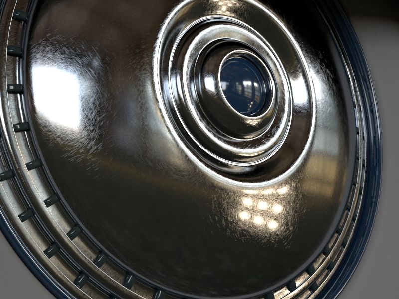
A. Atanasov, A. Wilkie, V. Koylazov & J. Křivánek / A Multiscale Microfacet Model Based on Inverse Bin Mapping

  σr              Yan (flat)                             Ours                                            Table 1: Table of notation.
                                                                                      Macrosurface-related symbols
                                                                                H2          Unit hemisphere
                                                                                D           Unit disk
                                                                                i           Incoming light direction
 0.01                                                                           o           Outgoing light direction
                                                                                n           Surface normal at position x
                                                                                h           Half vector h = (i + o)/ki + ok
                                                                                x           Position on a macrosurface
                                                                                A           Finite region in texture space around x
                                                                                 fx         Combined BRDF at position x
                                                                                 fA         Filtered BRDF over A
                                                                                F           Fresnel term for conductors or dielectrics

 0.05                                                                              Microsurface-related symbols:
                                                                                tk        Normal of k-th texel
                                                                                Tk        Texture space region corresponding to k-th texel
                                                                                N         Total number of normal map texels
                                                                                wk        Texel weight |A ∩ Tk |/|A|
                                                                                Hj        Bin on the hemisphere with index j
                                                                                B         Total number of bins
                                                                                Wj        Bin weight ∑k|tk ∈H j wk
                                                                                β, β−1    Binning strategy and its inverse
                                                                                B, B−1 Bin Map and Inverse Bin Map
 0.25                                                                           Dx        Normal distribution function (NDF)
                                                                                Gx        Shadowing-masking function of the normal map
                                                                                α         Beckmann flake roughness
                                                                                fα        Microfacet micro-BRDF aligned with the microsurface
                                                                                Dα        Microfacet distribution of the micro-BRDF
                                                                                Gα        Shadowing-masking function of the micro-BRDF
Figure 3: Shoes scene [ZGJ20]: Renders with Gaussian flat ele-
                                                                                C         Texel contribution function
ments (left column) [YHMR16] and with our method (right column).
The three rows show increasing roughness σr (0.01, 0.05, 0.25).
Note that the method of Yan et al. is designed to render specular                     Other symbols:
surfaces and does not conserve energy for increased roughness.                  |X|           Surface area of the region X
                                                                                IX            Indicator function of the region X
                                                                                δ             Spherical delta function
                                                                                σr            Yan’s intrinsic roughness [YHJ*14; YHMR16]
3. Background
We present the main constructs that we build on to develop our
filtering algorithms.                                                         Indeed microfacet materials without roughness have all facets
                                                                              aligned with the macrosurface: the microfacet distribution Dα be-
                                                                              comes a Dirac delta distribution, there is no shadowing-masking
3.1. Microfacet BRDF                                                          Gα = 1, and the expression is nonzero only when h = n.
The microfacet BRDF with specular microfacets [WMLT07] is:
                              F(i, h)Dα (h, n)Gα (i, o, h, n)                 3.2. Normal map
            f α (i, o, n) =                                   .     (1)
                                      4(i · n)(o · n)                         The normal map is a collection of N texels, each occupying an equal
We use similar notation to Walter et al. [WMLT07], see Table 1.               rectangular region Tk of unit texture space, and it is associated with
However, their definitions of the microfacet distribution D and the           a normal in tangent space tk ∈ H2 . Alternatively, the normals can
shadowing-masking function G depend implicitly on the macrosur-               be defined as points on the unit disk D [YHJ*14].
face normal n and the roughness parameter α - note that all angles                 The normal distribution function (NDF) based on the normal map
are defined with respect to n. For clarity of our derivation we make          is
both dependences explicit. Importantly, microfacet BRDFs approach                                                       N
the specular BRDF [WMLT07] as the roughness diminishes                                                   Dx (m) =      ∑ δ(tk , m)IT (x),                            (3)
                                                                                                                                         k

                                   F(i, h)δ(h, n)                                                                     k=1
                         α
                 lim f (i, o, n) =                .                 (2)
                 α→0                 4(i · h)2                                which is dependent on the texture space position x and ITk is the

                                                                                                                                                     © 2021 The Author(s)
                                                                                    Computer Graphics Forum © 2021 The Eurographics Association and John Wiley & Sons Ltd.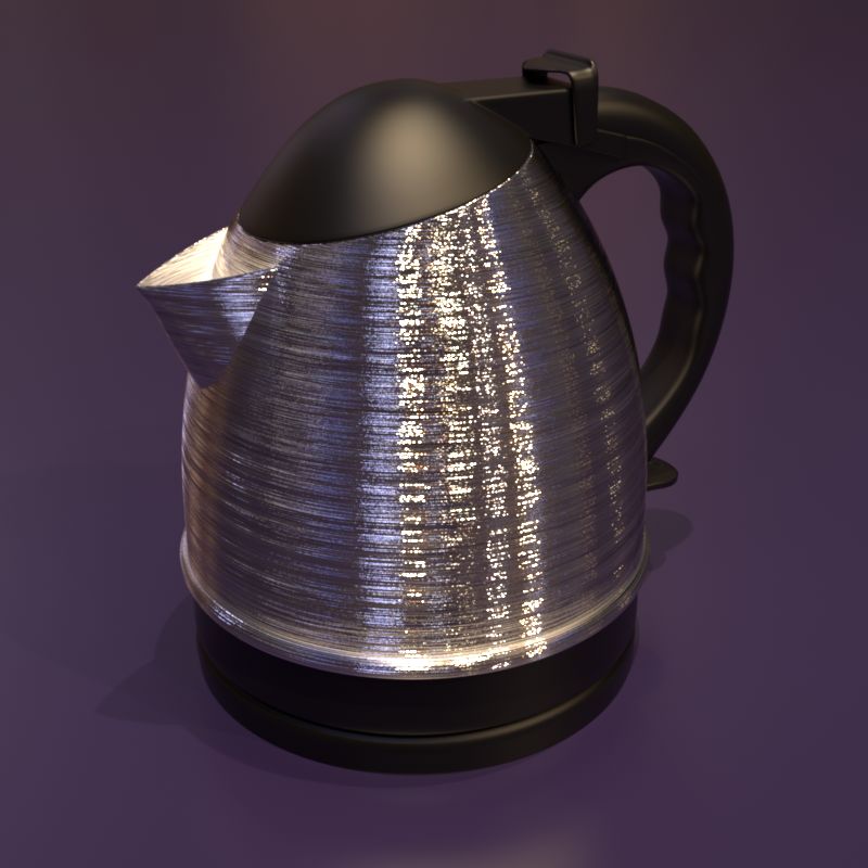
A. Atanasov, A. Wilkie, V. Koylazov & J. Křivánek / A Multiscale Microfacet Model Based on Inverse Bin Mapping

indicator function of the texel region Tk . Our definition is equivalent                       2D data set with specified binning strategy, the idea is to build SATs
to the one in Han et al. [HSRG07], however we do not divide                                    on the indicator functions of the bins[BP19]. Specifically, for a data
explicitly by N, because in our definition the texel area is |Tk | = N1 .                      set I with binning β the indicator functions are
                                                                                                                       (
                                                                                                                        1, β(I(i, j)) = b
3.3. Combined BRDF                                                                                         Ib (i, j) =                    , 0≤b≤B                  (8)
                                                                                                                        0, otherwise
In order to use microfacet BRDFs and normal maps together in                                   where B is the number of bins. The IH of the data set then is
a way that is in agreement with assumptions of microfacet theory
we follow a derivation similar to Schüssler et al. [SHHD17]. We                                                   IHI,β = {SATI0 , · · · , SATIB−1 }               (9)
substitute Dx for the microfacet distribution and f α for the micro                            Consequently, the histogram of any axis-aligned subregion of I can
BRDF in the general formula for microfacet BRDF with a micro                                   be extracted by evaluating Equation 7 for each bin.
BRDF assigned to each microfacet [WMLT07]
                                                                                                  In their original form, IHs are ideal due to their fast look-ups, but
                          (i · m)(o · m) α
                    Z
   fx (i, o, n) =                         f (i, o, m)Dx (m)Gx (i, o, m)dωm                     they have three considerable disadvantages:
                     H2    (i · n)(o · n)
                     N                                                                         • High memory requirements: the higher the number of bins the
                        (i · tk )(o · tk ) α                                                     sparser the bin indicator functions are. This redundancy increases
               =    ∑ (i · n)(o           f (i, o, tk )Gx (i, o, tk )ITk (x),
                    k=1
                                    · n)                                                         the memory footprint proportionally to the number of bins. There-
                                                                                         (4)     fore, it is not unusual for IHs to be unviable due to them exceeding
where n is the surface normal at position x, m is the microsurface                               the available memory for a given task[BP19].
normal and Gx is the shadowing-masking function corresponding to                               • Slow construction: the construction speed can be too slow for
Dx . As previous work, we use Smith shadowing-masking function                                   some applications, especially for large number of bins.
of the normal map Gx [YHMR16]. The integration is defined over                                 • Only axis-aligned look-ups: traditional IHs with fast look-up
the unit hemisphere H2 for an infinitesimal solid angle dωm around                               are restricted to axis-aligned rectangle regions. In turn, this would
the micronormal m. The delta function in the definition of Dx breaks                             imply that we would have to use axis-aligned pixel footprints A⊥ ,
the integral into a sum over all texel normals tk . Furthermore, only                            which is undesirable.
the term for which ITk (x) is nonzero, the term for which x ∈ Tk .
When we expand f α in this term we reach the desired combined                                  4. Normal map filtering
BRDF of a normal map and a microfacet BRDF
                                                                                               Proper filtering of normal maps is a challenging problem. In this
                (i · tk )(o · tk ) F(i, h)Dα (h, tk )Gα (i, o, h, tk )                         section, we analyse the filtering of our combined microfacet BRDF
 fx (i, o, n) =                                                        Gx (i, o, tk )
                (i · n)(o · n)             4(i · tk )(o · tk )                                 fx .
                  F(i, h)Dα (h, tk )Gα (i, o, h, tk )
              =                                       Gx (i, o, tk )
                          4(i · n)(o · n)                                                      4.1. Filtered BRDF
              = F(i, h)C(i, o, tk , n),                                                        We define the filtered BRDF fA by averaging a spatially varying
                                                                                         (5)   BRDF fx over a finite texture space region A around x:
where C(i, o, tk , n) = Dα (h, tk )Gα (i, o, h, tk )Gx (i, o, tk )/(4(i · n)(o ·                                                    1
                                                                                                                                         Z
                                                                                                                  fA (i, o, n) =               fx (i, o, n)dx.    (10)
n)) is the texel contribution.                                                                                                     |A|    A
                                                                                               Note that on both sides of the equation, n is the normal at position
3.4. Integral histogram (IH)                                                                   x. Like all previous filtering techniques we rely on the assumption
                                                                                               of a locally flat geometry. In practice this is a source of bias, which
For our exposition we describe 2D IHs, however they are directly                               is however sufficiently small when the surface normal n does not
generalized to higher dimensions. We start by defining the related                             change considerably over the region A. The filtered BRDF can be
concept of a summed-area table (SAT) [Cro84]. It is a cumulative                               defined more generally using an arbitrary filter kernel, but we use
table of a 2D array used for fast integral look-ups in arbitrary axis-                         the constant "box" filter |A|1
                                                                                                                              , because this will lead to an efficient
aligned regions. Given a 2D array I(i, j) ∈ R, the SAT of I is again
                                                                                               implementation later.
a 2D array of the same size
                                               i   j
                                                                                                  Using Equation 4 for fx we expand fA by substituting f α and
                           SATI (i, j) =                                                 (6)   distributing the integration over the normal map texels Tk
                                             ∑ ∑ I(k, l).
                                             k=0 l=0                                                                                     N
Given an arbitrary axis-aligned region i0 ≤ i ≤ i1 , j0 ≤ j ≤ j1 in I,                                        fA (i, o, n) = F(i, h) ∑ C(i, o, tk , n)wk ,        (11)
                                                                                                                                         k=1
the SAT is used to efficiently look up the sum of I over it
                                                                                               where
    SATI (i1 , j1 ) − SATI (i1 , j0 ) − SATI (i0 , j1 ) + SATI (i0 , j0 ).               (7)
                                                                                                                                    |A ∩ Tk |
                                                                                                                           wk =               .                   (12)
Note that this is a discrete application of the Fundamental Theorem                                                                   |A|
of Calculus in 2D.
                                                                                               Texel weights wk sum up to 1 and they are nonzero when the texels
   Integral Histograms (IHs) are a natural extension of SATs. For a                            Tk cover the filtering region A.

© 2021 The Author(s)
Computer Graphics Forum © 2021 The Eurographics Association and John Wiley & Sons Ltd.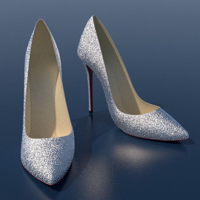
A. Atanasov, A. Wilkie, V. Koylazov & J. Křivánek / A Multiscale Microfacet Model Based on Inverse Bin Mapping

   Therefore, evaluation of this filtered BRDF requires a loop over
all normal map texels which happen to be fully or partially contained
in the filtering region A. For a small number of texels in A this                                                                  Tkj1 Tkj2
formulation is actually the most efficient way to compute the filtered                    Hj         h
BRDF, but as A grows to cover more texels, this formula becomes                                                                                    x         Tkj3
impractical. For such scenarios we derive alternative formulation
                                                                                                                                                Tkj4
for fA .
                                                                                                                                                           A
                                                                                                                                         Tkj5
4.2. Binned BRDF
We partition the hemisphere H2 into directional bins H j ⊂ H2 such
that Hi ∩ H j = ∅, for i 6= j and ∪Bj=1 H j = H2 , where B is the total        Figure 4: Left: The unit disk partitioned into 5 × 5 bins. The half
number of bins. Each normal from the map belongs to a bin tk ∈ H j             vector h is inside bin H j . Right: The pixel footprint A in the tex-
and therefore for a sufficiently fine binning all normals inside a bin         ture space. All 5 texels corresponding to the j-th bin B−1 ( j) =
are nearly identical. This allow us to group the terms in fA by bin            {k j1 , . . . , k j5 } are drawn in red. Three of them overlap with A, are
index j                                                                        in kA j , and contribute to W j .
                                       B
               fA (i, o, n) ≈ F(i, h) ∑ C(i, o, b j , n)W j ,       (13)
                                      j=1

where b j ∈ H j is a normal in bin j and the bin weights are W j =             we can evaluate Equation 13 by only considering a smaller number
∑k|tk ∈H j wk . Consequently, the bin weights W j also sum up to one           of bins B0 that sufficiently cover this cone:
like the texel weights wk . The bin weight represent what portion of                                                        B0
the surface in the region A has normal in a given bin.                                           fA (i, o, n) ≈ F(i, h) ∑ C(i, o, b j , n)W j                     (15)
                                                                                                                            j=1
  Note that if we build an IH of the normal map with a given binning
we can compute the bin weights W j in Equation 13 efficiently for
any axis-aligned region in texture space A⊥ , that additionally do not         5.2. Bin strategy
split texels.
                                                                               We partition the bounding square [−1, 1]2 of the unit disk D uni-
                                                                               formly into b × b bins, each with index j ∈ [0, b2 − 1], see Figure 4
5. Our solution                                                                (right). Each normal on the unit disk belongs to a bin and the bins
                                                                               that do not overlap with D are always empty (B ≤ b2 ). Then we can
There are practical concerns regarding direct use of Equation 13
                                                                               efficiently implement the binning function β and its inverse:
with an IH. Although, a single bin can be queried cheaply using
Equation 7, large number of bins can lead to a significant overhead.           • β(m) = j: Given a normal m ∈ H2 , we can find the in-
The other three practical challenges stem from the classical IH and              dex of the bin j which contains it: j = bb(0.5mx + 0.5)c +
are discussed in Section 3.4. In this section we address these issues            bbb(0.5my + 0.5)c.
and describe our filtering algorithm.                                          • β−1 ( j, ξ0 , ξ1 ) = m: We can sample a random normal inside
                                                                                 a given bin j: (mx , my ) = (2(b j%bc + ξ0 )/b − 1, 2(b j/bc +
                                                                                 ξ1 )/b − 1), where ξ0 and ξ1 are uniform random variables.
5.1. Beckmann flake roughness
                                                                               Our key idea is to choose the bin resolution b depending on the flake
First, we define the micro BRDF f α . We use the Beckmann micro-               roughness α in such way that the number of contributing bins B0
facet BRDF with Smith shadowing-masking function [WMLT07]                      is a small constant. Thus, surfaces with lower roughness will have
for Gα . The Beckmann microfacet distribution is                               higher bin resolutions. This can be done in a number of ways, but we
                                χ+ (h · tk )     − tan2 θ                      found that the following approach works well in practice. We take
               Dα (h, tk ) =                 exp          ,         (14)
                               πα2 cos4 (θ)         α2                         a square neighbourhood of bins centered at the bin which contains
                                                                               the half vector by taking two bins in each direction, a total of 25
where θ is the angle between h and tk , and χ+ (a) is one for a > 0            bins. Let the 3σ cone of radius sin(θ0 ) is centered around the half
and zero for a ≤ 0. It is a Gaussian distribution of slopes with stan-         vector (0, 0, 1). Our goal is to choose b so that the neighbourhood
dard deviation σ = √α [Hei14]. The tails of Dα are exponentially               of bins sufficiently covers this cone. We set b in such a way that the
                       2
bounded, and therefore, 95% of its microfacets are within 2σ and               ratio between the 25 neighbourhood bins and the total number of b2
nearly all of them are contained within 3σ. We chose the Beckmann              bins approximates the ratio between the area of the cone’s bounding
distribution with this property in mind, because the bin weights W j           square 4 sin2 (θ0 ) and the square of area 4 which bounds the unit
in Equation 13 do not need to be computed for all bins outside of              disk:
this region. These terms of the equation will be multiplied by the
                                                                                                                    5
tails of Dα and will have tiny contribution to the BRDF value. Given                                      b=                .                   (16)
                                                                                                                 sin(θ0 )
a threshold 3σ where we cut the tails, the truncated part of Dα lies in
a cone of angle θ0 = arctan(3σ) with radius sin(θ0 ). Subsequently,            Lastly, we omit the four corners of this square neighbourhood, be-

                                                                                                                                                    © 2021 The Author(s)
                                                                                   Computer Graphics Forum © 2021 The Eurographics Association and John Wiley & Sons Ltd.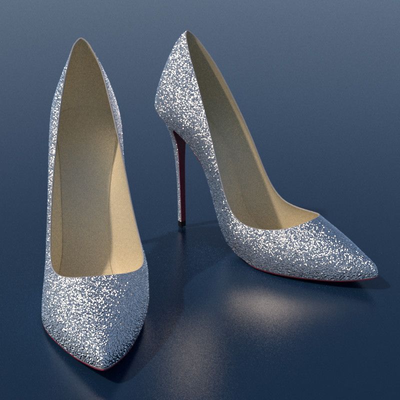
A. Atanasov, A. Wilkie, V. Koylazov & J. Křivánek / A Multiscale Microfacet Model Based on Inverse Bin Mapping

                                                                                           5.4. Inverse Bin Map
                                                                                           We developed a novel variant of IH data structures that we call
                                                                                           Inverse Bin Map. Its memory footprint and construction time are
                                                                                           practically independent of the number of bins. Additionally, it
                                                                                           natively supports arbitrary-shaped query regions. These critical
                                                                                           advantages come at the price of raising the look-up cost to
                                                                                           logarithmic, as with WaveletSAT.

                                                                                              A key observation is that in our context sampling and evaluation
                                                                                           are inverse operations. Sampling finds the incoming light direc-
Figure 5: Bin size vs. Beckmann flake roughness. Shown is a unit                           tion i of a given microsurface normal, while the evaluation finds
disk with entries for two half vectors (black dots), and their corre-                      all contributing microsurface normals given i. As usual, the inverse
sponding 3σ cones (blue). Left: bin resolution 12 × 12 for Beckmann                        problem is the harder of the two. We notice that sampling based
flake roughness α = 0.2 and Right: 34 × 34 for α = 0.07. See Table                         on the bin map B is a very efficient operation, while the evaluation
4 for the memory usage of our method for different bin resolutions.                        would require to loop over all bin map texels inside the filtering
                                                                                           region A. Potentially, this is inefficient since the number of texels
                                                                                           could be arbitrary large. Therefore, we designed a data structure that
                                                                                           can act as the inverse of the bin map, in order to make the reverse
cause they are mostly outside the 3σ cone and end up with B0 = 21,                         operation efficient. Since the bin map B maps a texel position to a
see Figure 5.                                                                              bin index, we define the inverse bin map B−1 as the mapping from
                                                                                           a bin index to the list of texel positions of all texels with the given
                                                                                           bin index:
5.3. Evaluation and sampling
                                                                                                B−1 ( j) = {k j1 , k j2 , · · · , k jn },   B(k ji ) = j,   i = 1..n   (19)
Using β we transform the input normal map into a bin map B, which
is an integer map of bin indices that correspond to each normal map                        where n is the total number of normal map normals in bin j. All lists
direction:                                                                                 of positions B−1 ( j) are concatenated in a single array of of size N
                                                                                           (note that |B−1 | = |B|). Essentially, a map of all bin (normal) map
                         B(k) = β(tk ) = j,          tk ∈ H j .                     (17)   positions, sorted by bin index.
Once the bin map is computed we do not store the original normal
map. All necessary components of our algorithm are based on B.                                We use B−1 to compute all bin weights W j by selecting the subset
We evaluate the BRDF as follows:
                                                                                           kA j of texels B−1 ( j) which lie in A: in Figure 4, only {k j2 , k j4 , k j5 }
• Find the bin of the half vector j = β(h)                                                 are in A. Note that in a typical normal map for some bins j |B−1 ( j)|
• Find all nearby B0 − 1 bins that belong to the neighbourhood of                          is too large for linear traversal. Therefore, we construct a 2D hier-
   j, see Figure 5                                                                         archy for each bin j such that |B−1 ( j)| > L, where L is a leaf size
• Compute all B0 bin weights W j of these bins                                             (L = 10 is our implementation), provided during construction.
• For all nonzero bin weights compute the texel contribution func-
  tion C at bin centers and accumulate the result, see Equation 15                            Two additional data structures accompany B−1 :
• Apply Fresnel term for conductors or dielectrics                                         Index I: Given a bin index it returns the size of B−1 ( j) and an
                                                                                           offset. For |B−1 ( j)|  L the offset is the start of
                                                                                           the 2D hierarchy in the forest F. I is implemented as an array of
• Sample random point in A
                                                                                           size B.
• Find the corresponding texel Tk
• Look up its bin index from the bin map j = B(k)                                             Forest F: A forest of 2D kd-trees, one for each bin j such that
• Compute the center normal of this bin b j = β−1 ( j, 0.5, 0.5)                           |B−1 ( j)| > L. During the construction of the forest we follow sev-
• Generate a random normal with Beckmann distribution m ∝ Dα                               eral conventions. First, we always split the larger side of the node in
  centered at b j                                                                          the middle, so that split dimension and split position do not need to
• Compute the reflected direction i = reflect(o, m)                                        be stored. Second, we sort each texel list so that for each tree node
                                                                                           its texels are consecutive in B−1 . This serves two purposes for the
The corresponding probability is
                                                                                           traversal: cache coherence is improved, and the size of each node
                                    1       B0                                             is implicitly propagated as offsets to the node start and end in B−1 .
                        p(i) =
                                 4(i · h)   ∑ Dα (h, b j )W j .                     (18)   This property provides pre-filtering data, so if a node is entirely
                                            j=1
                                                                                           inside the filtering region A its total area is immediately returned.
The rest of this section describes how we compute the bin weights                          Lastly, to achieve memory efficiency and to favour serialization, we
Wj.                                                                                        pack the whole forest topology in a single integer list.

© 2021 The Author(s)
Computer Graphics Forum © 2021 The Eurographics Association and John Wiley & Sons Ltd.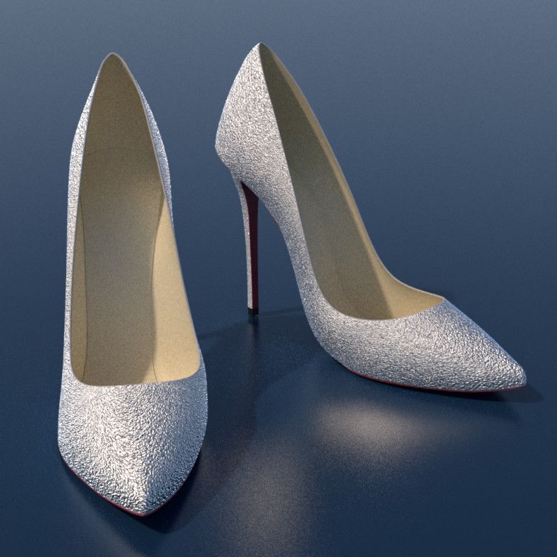
A. Atanasov, A. Wilkie, V. Koylazov & J. Křivánek / A Multiscale Microfacet Model Based on Inverse Bin Mapping

   Usually, IH are used to query the whole histogram with all B bins,
or as in our case sub-histogram of B0 bins together. The inverse bin
map is designed with this proposition in mind. Since all kd-trees
have the same splitting planes, hence the same node sizes. We imple-
ment traversal for a number of bins that computes the intersections
between tree nodes and the region A once for all queried bins. While
the tree nodes are axis-aligned, we use parallelogram approxima-
tion of the pixel footprint A based on ray differentials [Ige99]. In
principle, IBM can work with arbitrarily shaped query regions by
providing the proper node-region intersection procedures.

6. Results
We demonstrate our method with different normal maps and lighting
scenarios. We have implemented a car paint material with metallic
flakes, modelled with a normal map. Flakes orientations are sampled
from a GTR distribution [Bur12], and the corresponding Smith
shadowing-masking function is applied for Gx [Dim15]. The paint
consists of three layers: specular coat layer, metallic flakes layer
filtered with our algorithm and base layer with diffuse and glossy
term. The transparency of the flake layer is computed using a single
channel mip map; when we report the memory for our car paint
material we include this data structure in the total. Additionally, we
provide a control for the roughness of the individual flakes, as we
show in the Wing mirror scene, Figure 1. This scene is lit by a sun
and an environment light. In our video we show that for a range of
small Beckmann flake roughness values the filtering is crucial in
order to achieve converged result: renders with equal time stochastic
sampling exhibit severe flickering.
   Our second scene, the Car wheel (Figure 6) has 1K map with
scratches that are tiled over the surface to achieve a high texel-to-
pixel ratio. The scene is lit by 9 small area lights and an environment
with large light sources. In our video we observe that the portions of
the surface lit by the high frequency illumination (the 9 small lights)       Figure 6: Car wheel scene with scratch normal map and Beckmann
benefit from our filtering technique for low roughness values. As             flake roughness 0.01 (top) and 0.04 (bottom), and filtered with our
the roughness increases the filtered version is still more stable and         algorithm. The behaviour of this surface in an animation can be
some "boiling" can be seen in the stochastic version, however the             seen in the accompanying video: due to our pre-filtering, object
benefit of our technique for these scenarios is smaller.                      appearance is temporally stable across frames.

6.1. Comparison with previous work
We compare our method against Yan et al. [YHMR16], the current                texels per pixel grows, Yan’s curved elements convergence declines.
state of the art for rendering specular high-resolution normal maps.          Note that both Yan flat and curved elements use the same hierarchy
All comparison results in this subsection are based on the original           and intrinsic roughness. The difference in the performance in ×8
code, scenes and scripts provided by Zeltner et al. [ZGJ20], which            scenes (second and fourth row in Figure 7) is because in the curved
includes the original implementation of Yan et al. [YHMR16]. We               elements case there are 1-2 orders more contributing elements to
also implemented our own method as a Mitsuba 2 BRDF [NVZJ19].                 be processed in comparison with the flat elements case. We also
All comparisons were rendered on an AMD Ryzen Threadripper                    provide additional results from our method with increased rough-
3970X machine. As discussed in Section 2, we want to investigate              ness to demonstrate that our convergence is not impeded by growing
the scenario of increasing the number of texels that fall within a            number of contributing texels. In fact, it improves slightly. Addition-
typical image pixel. We do this by rendering the original scenes from         ally, the Shoes scene demonstrates that for some normal maps the
Zeltner et al.[ZGJ20], and by increasing the tiling of the input texture      appearance of Yan’s curved elements for low intrinsic roughness can
8 times which results in increasing the texel-to-pixel ratio 82 times.        be matched with our method with increased roughness, see Figure 7
The results from the comparisons are presented in Figure 7. Our               (the first two rows, Yan (curved) and Ours (rough)). Our method
method demonstrates very similar convergence rates to Yan’s flat              is 90× more memory efficient and the pre-processing is nearly 30×
elements for equal matched roughness σr = 0.005. The convergence              faster than Yan’s method with flat Gaussian elements, see Tables 2
plots for both scenes clearly show a tendency: as the number of               and 3. Our method has low memory requirements for wide range of

                                                                                                                                                   © 2021 The Author(s)
                                                                                  Computer Graphics Forum © 2021 The Eurographics Association and John Wiley & Sons Ltd.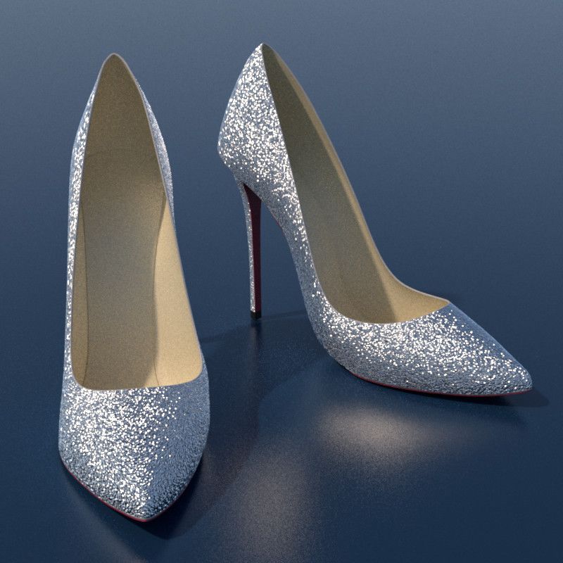
A. Atanasov, A. Wilkie, V. Koylazov & J. Křivánek / A Multiscale Microfacet Model Based on Inverse Bin Mapping

         Table 2: Memory usage for the methods in Figure 7.                                References
                                                                                           [Bli78] B LINN, JAMES F. “Simulation of Wrinkled Surfaces”. Proceedings
                        Ours        Yan (flat)       Yan (curved)           Ours (rough)      of the 5th Annual Conference on Computer Graphics and Interactive
  Shoes scene          36MB           3.2GB               19.3GB                  36MB       Techniques. SIGGRAPH ’78. New York, NY, USA: ACM, 1978, 286–
  Kettle scene         36MB           3.4GB                59GB                   36MB        292. DOI: 10.1145/800248.507101. URL: http://doi.acm.
                                                                                              org/10.1145/800248.507101.
                                                                                           [BP19] BALLESTER -R IPOLL, R. and PAJAROLA, R. “Tensor Decomposi-
     Table 3: Pre-processing times of the methods in Figure 7.                               tions for Integral Histogram Compression and Look-Up”. IEEE Transac-
                                                                                             tions on Visualization and Computer Graphics 25.2 (Feb. 2019), 1435–
                       Ours       Yan (flat)       Yan (curved)           Ours (rough)       1446. DOI: 10.1109/TVCG.2018.2802521.
  Shoes scene          0.2s            8.2s               56.6s                   0.3s     [BS63] B ECKMANN, P ETR and S PIZZICHINO, A NDRE. The Scattering
  Kettle scene         0.3s            8.4s              241.3s                   0.3s       of Electromagnetic Waves from Rough Surfaces. New York: Pergamon,
                                                                                             1963.
                                                                                           [Bur12] B URLEY, B RENT. “Physically-Based Shading at Disney”. 2012.
Beckmann flake roughness values, and therefore wide range of bin                           [BYRN17] B ELCOUR, L AURENT, YAN, L ING -Q I, R AMAMOORTHI, R AVI,
resolutions, see Table 4. For higher resolutions the index I takes                           and N OWROUZEZAHRAI, D EREK. “Antialiasing Complex Global Illu-
more memory, but the trees in the forest F are shallow and take less                         mination Effects in Path-Space”. ACM Trans. Graph. 36.4 (Jan. 2017).
                                                                                             ISSN : 0730-0301. DOI : 10.1145/3072959.2990495. URL : http:
memory. For lower resolutions it is the opposite.                                            //doi.acm.org/10.1145/3072959.2990495.
                                                                                           [CCM18] C HERMAIN, X AVIER, C LAUX, F RÉDÉRIC, and M ÉRILLOU,
7. Conclusion and future work                                                                S TÉPHANE. “A microfacet-based BRDF for the accurate and efficient
                                                                                             rendering of high-definition specular normal maps”. The Visual Computer
In this paper, we present a production-ready normal map filtering                            (Oct. 2018). DOI: 10.1007/s00371-018-1606-7.
method: there are no noticeable pre-computation times, and its mem-                        [Cro84] C ROW, F RANKLIN C. “Summed-area Tables for Texture Map-
ory requirements are very low. Due to pre-filtering being applied,                           ping”. Proceedings of the 11th Annual Conference on Computer Graph-
our technique does not slow down if large numbers of normal map                              ics and Interactive Techniques. SIGGRAPH ’84. New York, NY, USA:
texels fall within a single pixel: zooming out from a surface with                           ACM, 1984, 207–212. ISBN: 0-89791-138-5. DOI: 10.1145/800031.
                                                                                             808600. URL: http : / / doi . acm . org / 10 . 1145 / 800031 .
glints does not cause performance issues.                                                    808600.
   The algorithm we propose filters direct illumination. Our filter-                       [CSJD20] C HERMAIN, X AVIER, S AUVAGE, BASILE, J EAN -M ICHEL, D IS -
ing solution is based on an Inverse Bin Map: a specialized integral                          CHLER , and DACHSBACHER , C ARSTEN . “Procedural Physically-based
                                                                                             BRDF for Real-Time Rendering of Glints”. Comput. Graph. Forum (Proc.
histogram implementation that enables us to perform the neces-
                                                                                             Pacific Graphics) 39.7 (2020), 243–253.
sary lookups with low memory requirements, and at reasonable
                                                                                           [CT82] C OOK, R. L. and T ORRANCE, K. E. “A Reflectance Model for
speeds. We believe that this data structure has the potential to re-
                                                                                             Computer Graphics”. ACM Trans. Graph. 1.1 (Jan. 1982), 7–24. ISSN:
place IH in some applications where construction speed, memory                               0730-0301. DOI: 10.1145/357290.357293. URL: http://doi.
efficiency or regions with arbitrary shapes are important. Extending                         acm.org/10.1145/357290.357293.
the Inverse Bin Map to Gaussian queries would also benefit some                            [DHI*13] D UPUY, J ONATHAN, H EITZ, E RIC, I EHL, J EAN -C LAUDE, et al.
applications[BP19].                                                                          “Linear Efficient Antialiased Displacement and Reflectance Mapping”.
                                                                                             ACM Transactions on Graphics. Proceedings of Siggraph Asia 2013 32.6
                                                                                             (Nov. 2013), Article No. 211. DOI: 10.1145/2508363.2508422.
8. Acknowledgements                                                                          URL: https://hal.inria.fr/hal-00858220.

We dedicate this work to our friend and colleague Jaroslav. We                             [Dim15] D IMOV, ROSSEN. “Deriving the Smith shadowing function G1 for
                                                                                             γ ∈ (0, 4]”. 2015.
are grateful to Tashko Zashev for preparing the wing mirror scene
and to the anonymous reviewers for the insightful remarks, and                             [EKK99] E RSHOV, S ERGEY V., K HODULEV, A NDREI B., and KOLCHIN,
                                                                                             KONSTANTIN V. “Simulation of sparkles in metallic paints”. Proceedings
acknowledge academic funding from the following sources: GAČR                               of Graphicon’99. 1999, 121–128.
grant number 19-07626S, Charles University grant SVV-260588.
                                                                                           [EKM01] E RSHOV, S ERGEY, KOLCHIN, KONSTANTIN, and
                                                                                             M YSZKOWSKI, K AROL. “Rendering Pearlescent Appearance
                                                                                             Based On Paint-Composition Modelling”. Comput. Graph. Forum 20
Table 4: The bin resolution and memory usage of our method for                               (Sept. 2001). DOI: 10.1111/1467-8659.00515.
varying Beckmann flake roughness.                                                          [GCG*05] G ÜNTHER, J OHANNES, C HEN, T ONGBO, G OESELE,
                                                                                             M ICHAEL, et al. “Efficient Acquisition and Realistic Rendering of Car
  Beckmann roughness α                 0.0025          0.01         0.04         0.16        Paint”. 2005.
       Bin resolution b2                 9422         2352           592          152      [GGN18] G AMBOA, L UIS E., G UERTIN, J EAN -P HILIPPE, and
  Wing mirror scene (2K)               43MB          37MB         36MB         36MB          N OWROUZEZAHRAI, D EREK. “Scalable Appearance Filtering for
   Car wheel scene (1K)                15MB           9MB          9MB          8MB          Complex Lighting Effects”. ACM Trans. Graph. 37.6 (Dec. 2018), 277:1–
                                                                                             277:13. ISSN: 0730-0301. DOI: 10.1145/3272127.3275058. URL:
       Shoes scene (2K)                40MB          36MB         36MB         36MB          http://doi.acm.org/10.1145/3272127.3275058.
       Kettle scene (2K)               42MB          36MB         36MB         36MB
                                                                                           [Hei14] H EITZ, E RIC. “Understanding the Masking-Shadowing Function
                                                                                             in Microfacet-Based BRDFs”. Journal of Computer Graphics Techniques
                                                                                             (JCGT) 3.2 (June 2014), 48–107. ISSN: 2331-7418. URL: http : / /
                                                                                             jcgt.org/published/0003/02/03/.

© 2021 The Author(s)
Computer Graphics Forum © 2021 The Eurographics Association and John Wiley & Sons Ltd.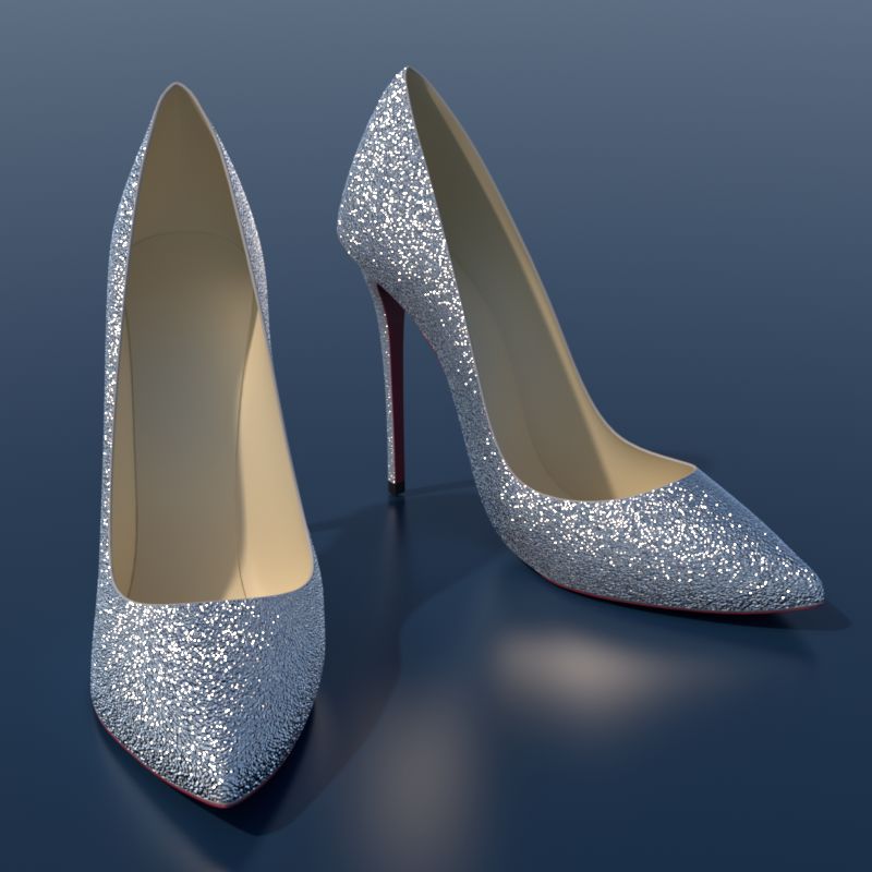
A. Atanasov, A. Wilkie, V. Koylazov & J. Křivánek / A Multiscale Microfacet Model Based on Inverse Bin Mapping

[HSRG07] H AN, C HARLES, S UN, B O, R AMAMOORTHI, R AVI, and G RIN -            [VG95] V EACH, E RIC and G UIBAS, L EONIDAS J. “Optimally Combining
  SPUN , E ITAN . “Frequency domain normal map filtering”. ACM Trans.             Sampling Techniques for Monte Carlo Rendering”. Proceedings of the
  Graph. 26 (July 2007), 28. DOI: 10.1145/1275808.1276412.                        22nd Annual Conference on Computer Graphics and Interactive Tech-
[Ige99] I GEHY, H OMAN. “Tracing Ray Differentials”. Proceedings of the           niques. SIGGRAPH ’95. New York, NY, USA: ACM, 1995, 419–428.
                                                                                  ISBN: 0-89791-701-4. DOI: 10.1145/218380.218498. URL: http:
   26th Annual Conference on Computer Graphics and Interactive Tech-
   niques. SIGGRAPH ’99. New York, NY, USA: ACM Press/Addison-                    //doi.acm.org/10.1145/218380.218498.
   Wesley Publishing Co., 1999, 179–186. ISBN: 0-201-48560-5. DOI: 10.          [VWH18] V ELINOV, Z DRAVKO, W ERNER, S EBASTIAN, and H ULLIN,
   1145 / 311535 . 311555. URL: http : / / dx . doi . org / 10 .                  M ATTHIAS B. “Real-Time Rendering of Wave-Optical Effects on
   1145/311535.311555.                                                            Scratched Surfaces”. Computer Graphics Forum 37 (2) (Proc. EURO-
                                                                                  GRAPHICS) 37.2 (2018).
[JHY*14] JAKOB, W ENZEL, H AŠAN, M ILOŠ, YAN, L ING -Q I, et al. “Dis-
   crete Stochastic Microfacet Models”. ACM Trans. Graph. 33.4 (July            [WHHY20] WANG, B EIBEI, H AŠAN, M ILOŠ, H OLZSCHUCH, N ICOLAS,
   2014), 115:1–115:10. ISSN: 0730-0301. DOI: 10 . 1145 / 2601097 .               and YAN, L ING -Q I. “Example-Based Microstructure Rendering with
   2601186. URL: http://doi.acm.org/10.1145/2601097.                              Constant Storage”. ACM Trans. Graph. 39.5 (Aug. 2020). ISSN: 0730-
   2601186.                                                                       0301. DOI: 10.1145/3406836. URL: https://doi.org/10.
                                                                                  1145/3406836.
[KHX*19] K UZNETSOV, A LEXANDR, H AŠAN, M ILOŠ, X U, Z EXIANG, et
  al. “Learning Generative Models for Rendering Specular Microgeometry”.        [Wil83] W ILLIAMS, L ANCE. “Pyramidal Parametrics”. SIGGRAPH Com-
  ACM Trans. Graph. 38.6 (Nov. 2019), 225:1–225:14. ISSN: 0730-0301.              put. Graph. 17.3 (July 1983), 1–11. ISSN: 0097-8930. DOI: 10.1145/
  DOI : 10.1145/3355089.3356525. URL : http://doi.acm.                            964967 . 801126. URL: http : / / doi . acm . org / 10 . 1145 /
  org/10.1145/3355089.3356525.                                                    964967.801126.
[LS13] L EE, T. and S HEN, H. “Efficient Local Statistical Analysis via Inte-   [WMLT07] WALTER, B RUCE, M ARSCHNER, S TEPHEN R., L I, H ONG -
  gral Histograms with Discrete Wavelet Transform”. IEEE Transactions             SONG , and T ORRANCE , K ENNETH E. “Microfacet Models for Refrac-
  on Visualization and Computer Graphics 19.12 (Dec. 2013), 2693–2702.            tion Through Rough Surfaces”. Proceedings of the 18th Eurographics
  DOI : 10.1109/TVCG.2013.152.                                                    Conference on Rendering Techniques. EGSR’07. Grenoble, France: Eu-
                                                                                  rographics Association, 2007, 195–206. ISBN: 978-3-905673-52-4. DOI:
[NVZJ19] N IMIER -DAVID, M ERLIN, V ICINI, D ELIO, Z ELTNER, T IZIAN,             10.2312/EGWR/EGSR07/195- 206. URL: http://dx.doi.
  and JAKOB, W ENZEL. “Mitsuba 2: A Retargetable Forward and Inverse              org/10.2312/EGWR/EGSR07/195-206.
  Renderer”. ACM Trans. Graph. 38.6 (Nov. 2019). ISSN: 0730-0301. DOI:
  10.1145/3355089.3356498. URL: https://doi.org/10.                             [WVJH17] W ERNER, S EBASTIAN, V ELINOV, Z DRAVKO, JAKOB, W EN -
  1145/3355089.3356498.                                                           ZEL , and H ULLIN , M ATTHIAS B. “Scratch Iridescence: Wave-optical
                                                                                  Rendering of Diffractive Surface Structure”. ACM Trans. Graph. 36.6
[OB10] O LANO, M ARC and BAKER, DAN. “LEAN Mapping”. Proceedings                  (Nov. 2017), 207:1–207:14. ISSN: 0730-0301. DOI: 10 . 1145 /
  of the 2010 ACM SIGGRAPH Symposium on Interactive 3D Graphics and               3130800.3130840. URL: http://doi.acm.org/10.1145/
  Games. I3D ’10. Washington, D.C.: ACM, 2010, 181–188. ISBN: 978-                3130800.3130840.
  1-60558-939-8. DOI: 10.1145/1730804.1730834. URL: http:
  //doi.acm.org/10.1145/1730804.1730834.                                        [WZYR19] W U, L IFAN, Z HAO, S HUANG, YAN, L ING -Q I, and R A -
                                                                                  MAMOORTHI , R AVI . “Accurate Appearance Preserving Prefiltering for
[Por05] P ORIKLI, FATIH. “Integral Histogram: A Fast Way To Extract               Rendering Displacement-Mapped Surfaces”. ACM Trans. Graph. 38.4
   Histograms in Cartesian Spaces”. Proceedings of the 2005 IEEE Com-             (July 2019). ISSN: 0730-0301. DOI: 10.1145/3306346.3322936.
   puter Society Conference on Computer Vision and Pattern Recognition            URL: https://doi.org/10.1145/3306346.3322936.
  (CVPR’05) - Volume 1 - Volume 01. Vol. 1. CVPR ’05. USA: IEEE Com-
   puter Society, July 2005, 829–836. ISBN: 0769523722. DOI: 10.1109/           [YHJ*14] YAN, L ING -Q I, H AŠAN, M ILOŠ, JAKOB, W ENZEL, et al. “Ren-
   CVPR.2005.188. URL: https://doi.org/10.1109/CVPR.                              dering Glints on High-Resolution Normal-Mapped Specular Surfaces”.
   2005.188.                                                                      ACM Transactions on Graphics (Proceedings of SIGGRAPH) 33.4 (July
                                                                                  2014), 116:1–116:9. DOI: 10.1145/2601097.2601155.
[RGB16] R AYMOND, B ORIS, G UENNEBAUD, G AEL, and BARLA, PAS -
  CAL . “Multi-Scale Rendering of Scratched Materials using a Structured
                                                                                [YHMR16] YAN, L ING -Q I, H AŠAN, M ILOŠ, M ARSCHNER, S TEVE, and
  SV-BRDF Model”. ACM Transactions on Graphics (July 2016). DOI:                  R AMAMOORTHI, R AVI. “Position-Normal Distributions for Efficient
  10 . 1145 / 2897824 . 2925945. URL: https : / / hal . inria .                   Rendering of Specular Microstructure”. ACM Transactions on Graphics
  fr/hal-01321289.                                                                (Proceedings of SIGGRAPH 2016) 35.4 (2016).

[RMS*08] RUMP, M ARTIN, M ÜLLER, G ERO, S ARLETTE, R ALF, et al.                [YHW*18] YAN, L ING -Q I, H AŠAN, M ILOŠ, WALTER, B RUCE, et al.
  “Photo-realistic Rendering of Metallic Car Paint from Image-Based               “Rendering Specular Microgeometry with Wave Optics”. ACM Trans.
  Measurements”. Computer Graphics Forum 27.2 (Apr. 2008). Ed. by                 Graph. 37.4 (July 2018), 75:1–75:10. ISSN: 0730-0301. DOI: 10.1145/
  S COPIGNO, R. and G RÖLLER, E., 527–536.                                        3197517.3201351. URL: http://doi.acm.org/10.1145/
                                                                                  3197517.3201351.
[SHHD17] S CHÜSSLER, V INCENT, H EITZ, E RIC, H ANIKA, J OHANNES,
                                                                                [ZGJ20] Z ELTNER, T IZIAN, G EORGIEV, I LIYAN, and JAKOB, W ENZEL.
  and DACHSBACHER, C ARSTEN. “Microfacet-Based Normal Mapping
                                                                                  “Specular Manifold Sampling for Rendering High-Frequency Caustics
  for Robust Monte Carlo Path Tracing”. ACM Trans. Graph. 36.6 (Nov.
                                                                                  and Glints”. ACM Trans. Graph. 39.4 (July 2020). ISSN: 0730-0301. DOI:
  2017). ISSN: 0730-0301. DOI: 10.1145/3130800.3130806. URL:
                                                                                  10.1145/3386569.3392408. URL: https://doi.org/10.
  https://doi.org/10.1145/3130800.3130806.
                                                                                  1145/3386569.3392408.
[SNM*02] S UNG, L I -P IIN, NADAL, M ARIA E., M C K NIGHT, M ARY E.,
                                                                                [ZK16] Z IRR, T OBIAS and K APLANYAN, A NTON S. “Real-time Render-
  et al. “Optical reflectance of metallic coatings: Effect of aluminum flake
                                                                                  ing of Procedural Multiscale Materials”. Proceedings of the 20th ACM
  orientation”. Journal of Coatings Technology 74 (2002). ISSN: 1935-3804.
                                                                                  SIGGRAPH Symposium on Interactive 3D Graphics and Games. I3D ’16.
  URL : https://doi.org/10.1007/BF02697975.
                                                                                  Redmond, Washington: ACM, 2016, 139–148. ISBN: 978-1-4503-4043-4.
[Tok05] T OKSVIG, M ICHAEL. “Mipmapping Normal Maps”. Journal                     DOI : 10.1145/2856400.2856409. URL : http://doi.acm.
   Graphics Tools 10 (2005), 65–71.                                               org/10.1145/2856400.2856409.
[TS67] T ORRANCE, K.E. and S PARROW, E.M. “Theory for Off-Specular              [ZXW19] Z HU, J UNQIU, X U, YANNING, and WANG, L U. “A Stationary
  Reflection from Roughened Surfaces”. Journal of the Optical Soci-               SVBRDF Material Modeling Method Based on Discrete Microsurface”.
  ety of America (JOSA) 57.9 (Sept. 1967), 1105–1114. URL: http :                 Computer Graphics Forum 38.7 (2019), 745–754. DOI: 10.1111/cgf.
  / / www . graphics . cornell . edu / ~westin / pubs /                           13876. URL: https : / / onlinelibrary . wiley . com / doi /
  TorranceSparrowJOSA1967.pdf.                                                    abs/10.1111/cgf.13876.

                                                                                                                                                     © 2021 The Author(s)
                                                                                    Computer Graphics Forum © 2021 The Eurographics Association and John Wiley & Sons Ltd.
A. Atanasov, A. Wilkie, V. Koylazov & J. Křivánek / A Multiscale Microfacet Model Based on Inverse Bin Mapping
Ours Yan (flat) Yan (curved) Ours (rough) Ours Yan (flat) Yan (curved) Ours (rough)
x1 100 100
Convergence plot: RMSE over time [s]
Ours Ours
100 100
Convergence plot: RMSE over time [s]
Ours Ours
Yan (flat)Yan (flat) Yan (flat)Yan (flat)
Yan (curved)
Yan (curved) Yan (curved)
Yan (curved)
10−1 10−1 Ours (rough)
Ours (rough) 10−1 10−1 Ours (rough)
Ours (rough)
10−2 10−2 10−2 10−2
−3 −3
10 10 10−3 10−3
100 100 101 101 102 102 103 103 100 100 101 101 102 102 103 103
Ours Yan (flat) Yan (curved) Ours (rough) Ours Yan (flat) Yan (curved) Ours (rough)
x8 100 100
Convergence plot: RMSE over time [s]
Ours Ours
100 100
Convergence plot: RMSE over time [s]
Ours Ours
Yan (flat)Yan (flat) Yan (flat)Yan (flat)
Yan (curved)
Yan (curved) Yan (curved)
Yan (curved)
10−1 10−1 Ours (rough)
Ours (rough) 10−1 10−1 Ours (rough)
Ours (rough)
10−2 10−2 10−2 10−2
−3 −3
10 10 10−3 10−3
100 100 101 101 102 102 103 103 100 100 101 101 102 102 103 103
Ours Yan (flat) Yan (curved) Ours (rough) Ours Yan (flat) Yan (curved) Ours (rough)
x1 Convergence plot: RMSE over time [s]
Ours Ours
Convergence plot: RMSE over time [s]
Ours Ours
Yan (flat)Yan (flat) Yan (flat)Yan (flat)
100 100 Yan (curved)
Yan (curved) 100 100 Yan (curved)
Yan (curved)
Ours (rough)
Ours (rough) Ours (rough)
Ours (rough)
10−1 10−1 10−1 10−1
10−2 10−2 10−2 10−2
100 100 101 101 102 102 103 103 100 100 101 101 102 102 103 103
Ours Yan (flat) Yan (curved) Ours (rough) Ours Yan (flat) Yan (curved) Ours (rough)
x8 Convergence plot: RMSE over time [s]
Ours Ours
Convergence plot: RMSE over time [s]
Ours Ours
Yan (flat)Yan (flat) Yan (flat)Yan (flat)
100 100 Yan (curved)
Yan (curved) 100 100 Yan (curved)
Yan (curved)
Ours (rough)
Ours (rough) Ours (rough)
Ours (rough)
10−1 10−1 10−1 10−1
10−2 10−2 10−2 10−2
100 100 101 101 102 102 103 103 100 100 101 101 102 102 103 103
Figure 7: Shoes and Kettle scenes (800 × 800) [ZGJ20]: We render two different texture tiles - the original scenes in the first and third
rows and then ×8 tiles in the second and fourth rows. All of these scenarios were rendered with four variations: our method, Yan et al. flat
elements, Yan et al. curved elements, and our method with slightly increased roughness. The first three variations have equal roughness values
σr = 0.005, while the last demonstrates our method with higher Beckmann flake roughness α = 0.05 (σr = √α ) that is not supported by Yan’s
2
method. The large images in the left column are rendered with our low roughness variant (the first variant labelled Ours). Two regions of
size 80x80 are selected from both scenes, and convergence plots are computed for each of them (middle and right column). We use the script
provided by Zeltner et al. [ZGJ20] to compute the plots.
© 2021 The Author(s)
Computer Graphics Forum © 2021 The Eurographics Association and John Wiley & Sons Ltd.You can also read