Inferring Road Maps from Global Positioning System Traces
←
→
Page content transcription
If your browser does not render page correctly, please read the page content below
Inferring Road Maps from Global
Positioning System Traces
Survey and Comparative Evaluation
James Biagioni and Jakob Eriksson
As a result of the availability of Global Positioning System (GPS) sensors difficult to understand the relative merits of the various proposed
in a variety of everyday devices, GPS trace data are becoming increas- map inference methods.
ingly abundant. One potential use of this wealth of data is to infer and The lack of quantitative, comparative evaluations of map inference
update the geometry and connectivity of road maps through the use of algorithms is attributable to three missing ingredients: (a) sufficiently
what are known as map generation or map inference algorithms. These expressive and robust methods of quantitatively evaluating the accu-
algorithms offer a tremendous advantage when no existing road map racy of a generated map, (b) publicly available implementations of
data are present. Instead of the expense of a complete road survey, proposed map inference methods, and (c) common sets of publicly
GPS trace data can be used to generate entirely new sections of the available GPS traces and ground truth maps for use in evaluations.
road map at a fraction of the cost. In cases of existing maps, road map In this paper, the three problems identified earlier are thoroughly
inference may not only help to increase the accuracy of available road addressed. The research (a) describes the first quantitative evaluation
maps but may also help to detect new road construction and to make method for map inference algorithms, (b) provides open source imple-
dynamic adaptions to road closures—useful features for in-car naviga- mentations of three reference algorithms, and (c) makes available a
tion with digital road maps. In past research, proposed algorithms had 118-h trace data set, plus ground truth maps, for unrestricted use by the
been evaluated qualitatively with little or no comparison with prior work. map inference community. The data and implementations are available
This lack of quantitative and comparative evaluation is addressed in this on the BITS laboratory website (2). To provide a better understanding
paper with the following contributions: (a) a comprehensive survey of of prior work on map inference, the following are also provided: (a) a
the current literature on map generation; (b) a description of the first comprehensive survey of the current literature on automatic map gen-
method for the automatic evaluation of generated maps; (c) a qualitative, eration and (b) a qualitative, quantitative, and c omparative evaluation
quantitative, and comparative evaluation of three reference algorithms; of the three reference algorithm implementations.
and (d) an open source implementation of each of the three algorithms, The remainder of the paper is structured as follows: (a) a survey of
with a 118-h trace data set and ground truth map for unrestricted use by the literature on the topic of automatic map generation, which briefly
the automatic map generation community. describes the various methods proposed and the evaluation performed
in each paper; (b) a description of the proposed quantitative evaluation
method; (c) a visual illustration of the performance of the algorithms
Road map inference is the process of automatically producing a and qualitative observations; (d) an analysis of the quantitative mea-
directed, annotated road map from GPS traces. GPS traces are typi- sures of the performance and a brief discussion of the implementations
cally collected opportunistically, from vehicles that are driving the of three reference algorithms (3–5); and (e) conclusions.
roads for some other purpose. Map inference can be used to rap-
idly map unknown or constantly changing territory, to update and
improve on existing road maps, or to quickly adapt to detours and Background and Survey
new construction. of Existing Literature
Common throughout the existing literature on automatic map gen-
eration is a focus on qualitative evaluation. Virtually every published The baseline requirement of a map inference algorithm is to auto-
paper on the topic relies on a visual inspection of the results and matically turn raw GPS traces into a directed and annotated graph
manually compares generated maps with existing maps or satellite that represents the connectivity and geometry of the underlying road
imagery. Moreover, comparisons with existing work are virtually network. Beyond such basic map generation, various additional
absent: out of 11 papers surveyed, only one provided any com- objectives have been proposed, such as the extraction of detailed
parison with prior work (1). The focus on qualitative evaluation in intersection geometries (6), the number and centerlines of lanes (6),
the literature, and the lack of comparative evaluation, has made it and the speed limit and road type (7). This paper focuses primarily on
basic map generation and only briefly mentions these other aspects.
Department of Computer Science, University of Illinois at Chicago, SEO 1120
M/C 152, 851 South Morgan Street, Chicago, IL 60607. Corresponding author:
J. Biagioni, jbiagi1@uic.edu. Operational Overview
Transportation Research Record: Journal of the Transportation Research Board,
No. 2291, Transportation Research Board of the National Academies, Washington,
The map generation process is typically preceded by a filtering step,
D.C., 2012, pp. 61–71. in which traces are checked for any irregularities with regard to the
DOI: 10.3141/2291-08 expected distance between points, the speed traveled, the acceleration,
61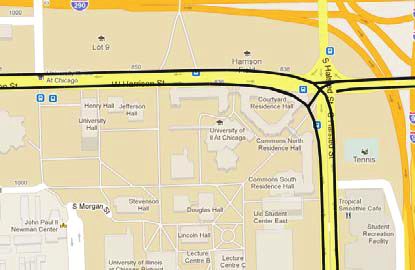
62                                                                                                             Transportation Research Record 2291

and any abrupt direction changes. Any point along a GPS trace that              Map Inference Based on k-Means Algorithm
fails to satisfy these criteria is removed, and an interpolated point is
inserted in its place.                                                          The k-means based approach, originally described in Edelkamp
   After filtering, the approaches described in the literature can be           and Schrödl (3), and illustrated in Figure 1, begins by distributing a
categorized by their algorithmic foundations: the k-means algorithm             series of cluster seeds at locations drawn from the set of trace data,
(8), trace merging, or kernel density estimation (KDE) (9). Mem-                with the constraint that every trace point must be within a fixed
bers of the first category perform variations on a three-dimensional            distance d and bearing difference δ of a cluster seed.
(latitude, longitude, direction) k-means algorithm to reduce the set               The cluster seeds are used as initial guesses; minor variations on
of GPS points to a smaller set of cluster centroids. The centroids              the k-means algorithm are then used to find the seed locations and
are then linked together to form the road geometry. Trace-merging               headings that best describe the raw traces. Once the seed locations
methods merge edges directly, without first reducing the set of raw             are identified, seeds are linked to form road segments, based on the
GPS data. Finally, KDE-based methods first produce a KD esti-                   pattern of raw traces passing through the seed locations. Qualita-
mate of the raw GPS points or edges, then co-opt image processing               tive and quantitative evaluations of the basic k-means algorithm are
techniques to extract the road geometry from this density estimate.             provided later in the current paper.

Survey of Existing Literature                                                   Edelkamp and Schrödl, 2003 (3)

Table 1 is a summary of the literature on automatic map generation.             In addition to being the original k-means based method, the 2003 paper
Out of the 11 papers, six report k-means based methods, two report              by Edelkamp and Schrödl further refines the road network model by
trace-merging methods, and three report KDE methods. As noted                   fine-tuning the location of intersections, representing the road center-
in the evaluation method column, the literature thus far has almost             line by a fitted spline rather than a series of straight lines, and perform-
exclusively relied on a qualitative evaluation method (eyeballing);             ing lane finding. Lane finding is done by clustering raw traces based on
only four papers quantitatively evaluated the accuracy of the gener-            their respective distance offset from the road centerline.
ated maps, and none made quantitative comparisons with existing                    This work was evaluated by comparing the number of lanes detected
work. Typically, a sample of the generated road geometry is overlaid            and the lane position error with a base map generated by the authors,
onto a map or satellite image (ground truth), from which conclusions            through the use of survey-grade differential GPS equipment.
are drawn manually. Despite the widespread availability of ground
truth maps, quantitative evaluation has been exceedingly rare in this
line of work. In cases in which any type of numerical accuracy result           Schroedl et al., 2004 (6)
has been reported, no comparison has been made with related work
(3, 6, 7, 11). Similarly, in cases in which a comparison has been made          Based on Edelkamp and Schrödl (3), the 2004 paper by Schroedl
with related work, only a qualitative comparison was offered, with              et al. describes a process for additionally refining the intersection
no numbers reported (1).                                                        geometry and modeling individual lanes and the transitions and turn
   In the following section, the three categories of map inference              restrictions between them. This process is accomplished by first
algorithms are introduced in more detail and the variations on each             identifying intersections and their bounding boxes. Traces through
offered in the literature are briefly discussed.                                an intersection are then grouped by entry and exit points, and a

TABLE 1   Chronological Summary of Papers on Map Inference

Paper                        Class           Data                          Ground Truth       Evaluation Method                     Features

Edelkamp and Schrödl (3)     k-means         250 synthetically             Generated from     Lane error vs. amount of data         Lane finding
                                               perturbed traces              GPS traces
Schroedl et al. (6)          k-means         250 synthetically             Generated from     Lane error vs. amount of data         Intersection geometry
                                               perturbed traces              GPS traces
Davies et al. (4)            KDE             1 million GPS points          UK ordnance        Eyeball vs. ground truth              na
                                                                             survey
Worrall and Nebot (10)       k-means         Traces from mining            None               Compact vs. raw                       Compact representation
                                                vehicles
Guo et al. (11)              k-means         Synthetic GPS traces          None               Relative error vs. amount of data     na
Chen and Cheng (12)          KDE             Traces from automobiles       Google Earth       Eyeball vs. ground truth              na
Niehoefer et al. (7)         Trace merge     7 traces                      Google Maps        Eyeball vs. ground truth, relative    Edge classification
                                                                                                error vs. amount of data
Cao and Krumm (5)            Trace merge     20 million GPS points         Bing Maps          Eyeball vs. ground truth, route       GPS trace clarification
                                                from campus shuttles                            query vs. Bing Maps
Shi et al. (13)              KDE             Massive amounts of GPS        Google Earth       Eyeball vs. ground truth              na
                                                traces
Jang et al. (14)             k-means         GPS traces                    Naver maps (15)    Eyeball vs. ground truth              na
Agamennoni et al. (1)        k-means         5 days or 15 open mine        None               Eyeball vs. Davies et al. (4) and     Principal road path
                                                vehicle GPS traces                              Schroedl et al. (6)

Note: na = not applicable.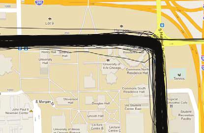
Biagioni and Eriksson                                                                                                                         63

                                     (a)                                                                   (b)

                                     (c)                                                                   (d)

   FIGURE 1   Map inference with k-means algorithm: (a) raw traces, (b) initial seeds, (c) updated means with bearing,
   and (d) final graph after means are linked.

spline-fitting technique (16) is used for each group to produce the         Map Inference Based on Trace Merging
final turn-lane geometry of the intersection.
   This work was evaluated by visually comparing generated inter-           The trace-merging methods proposed thus far use a greedy approach,
section geometries against Navteq maps (17). A heuristic perfor-            illustrated in Figure 2. Through iterations of each recorded GPS
mance optimization for this method was described by Jang et al. and         trace, edges from the raw trace are added to the map unless an edge
evaluated by visually comparing the generated map with the map              sufficiently similar in location and bearing already exists. Should
provided by the South Korean web portal Naver (14, 15).                     such an edge already exist, its weight is instead incremented. In
                                                                            postprocessing, any edges with weights below a certain threshold
                                                                            are removed.
Worrall and Nebot, 2007 (10)

In Worrall and Nebot, a method based on Edelkamp and Schrödl                Cao and Krumm, 2009 (5)
(3) is presented to infer a road network represented as a compact set
of lines and arcs. To create a compact representation of the gener-         The method proposed by Cao and Krumm (5) precedes the standard
ated road map, the set of clusters is first segmented into regions of       trace-merging method with a clarification step. The “clarification
constant curvature. The best line or arc is then fitted to each seg-        step” is a type of particle simulation, in which a strong but short-
ment. Standard regression analysis is used for regions that represent       range attractive force is applied to pull together nearby traces, and
straight lines; regions that represent arcs are fitted using nonlinear      a weaker but long-range retractive force is used to keep traces from
least-squares fitting (18).                                                 straying too far from their original location (21). This reduces the
   This work was evaluated by measuring the differences between             effects of GPS noise by pulling together traces that originate from the
the compressed map and the originally generated map. A similar              same road, thereby forming tight bands along the road centerlines.
approach is presented in Guo et al. (11).                                      This work was evaluated by visually comparing the generated
                                                                            map with satellite imagery from Bing Maps, and also by visually
                                                                            comparing shortest path routes from the generated map with those
Agamennoni et al., 2011 (1)                                                 from Bing Maps. Qualitative and quantitative evaluations of this
                                                                            trace-merging algorithm are provided later in the current paper.
The approach taken by Agamennoni et al. (1) is similar to Schroedl
et al. (6), but the focus is to extract “principal road paths,” which are
curves as defined in Hastie and Stuetzle (19).                              Niehoefer et al., 2009 (7)
   In Agamennoni et al. (20), a visual comparison is made against
the original k-means approach (6), as well as one based on KDE (4).         The method described by Niehoefer et al. modifies the standard
A limited quantitative evaluation of this method is also presented in       merging approach by adjusting the position of existing road seg-
Agamennoni et al., in which a GPS trace data set collected by the           ments when merging a new trace segment into the existing map (7).
authors is used (20).                                                       This technique allows the location of road segments in the base map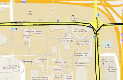
64                                                                                                     Transportation Research Record 2291

                                    (a)                                                                   (b)

                                    (c)                                                                   (d)

   FIGURE 2   Trace-merging approach: (a) raw GPS traces, (b) new edges added, (c) weights of matching edges incremented,
   and (d) edges with insufficient weight removed.

to be steadily refined as more traces are added, in a similar spirit to   Davies et al., 2006 (4)
the clarification preprocessing step used in Cao and Krumm (5),
except here it is used during the merge procedure. The paper also         In the scheme proposed by Davies et al., edges are accounted for in
describes means of automatically classifying road types, such as          each grid cell that they pass through by an amount proportional to the
highways, streets, or walkways, as well as entry and exit ramps,          length of the line between the two points that passes through the cell
bridges, and tunnels.                                                     in the antialiasing process (in computer graphics, “antialiasing” is
   A qualitative evaluation of this work was conducted by visually        the process of removing or reducing the jagged distortions in curves
comparing the generated map with the same region depicted in              and diagonal lines so that the lines become more smooth) (4, 23).
Google Maps. A quantitative evaluation was also performed against            After thresholding the density estimate (in computer graphics,
a reference map that was generated using all available traces,            “thresholding” is the process of converting an image into a binary
whereby the relative position error of a road segment was shown to        representation whereby pixels are marked as “object” pixels if their
rapidly decrease with increasing amounts of data.                         value is greater than a certain threshold and as “background” pixels
                                                                          if their value is lower than the threshold), the outlines of the pro-
                                                                          duced road bitmap image are extracted using a contour follower
Map Inference Based on KDE                                                (24). To find the centerlines of these outlines, which are likely to
                                                                          coincide with the centerlines of the underlying roads, the Voronoi
Map inference methods based on KDE (a) compute an approximate             graph of points, evenly spaced along the contours, is produced (25),
KD estimate of trace points or edges over the area of interest (9),       followed by the removal of edges that fall outside the contour or
(b) apply a threshold to produce a binary image of the roads, and         that are of insufficient length. Finally, separately produced KDEs of
(c) apply a variety of methods to produce road centerlines from this      traces in each of the eight cardinal and ordinal directions are used to
binary image, as illustrated in Figure 3.                                 annotate each road segment with its permitted directions of travel.
   To produce the KD estimate, the geographical area of interest             This work was evaluated by visually comparing the generated map
is divided into a two-dimensional grid of cells whose width is a          against that of a UK Ordnance Survey. Qualitative and quantitative
fraction of the road width. Through iterations over each of the raw       evaluations of this KDE-based algorithm are provided later in the paper.
GPS points or edges, a two-dimensional histogram is produced that
contains the number of points or edges that fall into each grid cell.     Chen and Cheng, 2008 (12)
The histogram is then convolved with a Gaussian smoothing func-
tion (22), producing an approximation of the desired KD estimate.         The KDE-based method described by Chen and Cheng produces a
This is an approximation because of the discretization created by the     point-based density estimate and takes an image-processing approach
use of grid cells, and the accuracy of the approximation is inversely     to extract the road map from the bitmap image produced after the
proportional to the grid size.                                            thresholding step (12). Morphological dilation and closing operations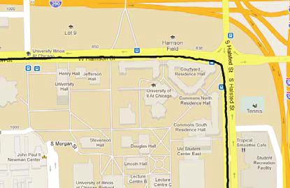
Biagioni and Eriksson 65
(a) (b)
(c) (d)
FIGURE 3 Map inference based on KDE (4): (a) raw traces, (b) KDE computed, (c) threshold applied and road or nonroad cells identified,
and (d) road outlines and centerlines computed.
are used to produce a smooth and contiguous image of the road bound- morphism (27), and inexact methods for measuring graphs’ editing
aries. Then, a thinning operation deletes all pixels on the boundaries distance (28). However, the problem of measuring the similarity of
of the pattern until only a skeleton remains along the road centerlines, graphs is fundamentally different from that of measuring the similarity
which is then converted into road segments. A very similar method was of maps: crucially, graphs and their nodes and edges lack any notion
proposed by Shi et al. (13). Both methods were evaluated by visually of geographical location. Thus, although graph similarity algorithms
comparing the generated maps with images from Google Earth. are able to measure the degree of topological similarity, the graphs’
nodes and edges can be freely transposed to find the closest match. In
a map, however, the geographical location of the nodes and edges must
Robust Quantitative Evaluation be taken into account, in addition to their topological relationships.
of Generated Maps To simultaneously measure the geometric and topological simi-
larity of maps, a method is proposed based on the following idea:
In this section, a method of evaluating the accuracy of a map, with starting from a random street location, explore each map outward
respect to a ground truth map, is described. This is a necessary within a maximum radius. This produces two sets of locations,
requirement for a quantitative, comparative evaluation of competing which are essentially spatial samples of a local map neighborhood.
map inference algorithms. Through a comparison of the two sets of samples and repeated sam-
The accuracy of a generated map depends on two primary aspects of pling of the maps, in this fashion, a robust measure of the difference
the map: geometry and topology. The geometry of the map describes between the two maps is obtained. If one of the maps is the ground
the geographical location of the roads, and the topology describes the truth, this difference represents the accuracy of the other map.
interconnections between the roads. The operation of the map comparison algorithm presented in this
A large body of work looks at the problem of comparing graphs paper is depicted in Figure 4. First, a start location is selected at
(26). This work includes exact methods for testing for graph iso- random from the ground truth map. This point is marked with an X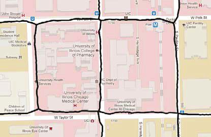
66 Transportation Research Record 2291
(a) (b) (c)
FIGURE 4 Overview of map comparison algorithm: (a) holes dropped at fixed intervals (ground truth map), (b) marbles dropped at fixed
intervals (generated map), and (c) marbles fill holes where maps overlap.
in Figure 4a. From the start location, all road segments within a small ity to capture the connectivity of the maps at a very detailed level
matching distance d are followed and virtual holes are dropped at fixed (i.e., as they would be traveled), allowing the topological similarity
intervals until a maximum radius r from the start location is reached or to be measured. Conversely, if a global approach to this problem were
a previously followed segment is encountered. When an intersection taken, in which every edge in the ground truth map was simply cov-
is encountered, all connecting road segments that lead away from the ered with holes, and every edge in the generated map with marbles,
start location are followed, as turn restrictions and one-way streets yielding just two sets to be matched, the process would capture the
allow. Restricting the process to segments leading away from the start geometric similarity between maps; however, it would fail to capture
location elegantly de-emphasizes unlikely driving patterns, such as local topological similarity, a crucial aspect of overall map similar-
U-turns, and improves the robustness of the map comparison opera- ity. Repeated local sampling at randomly chosen locations yields an
tion. This process is then repeated, starting from the road segments accurate view of local geometry and topology throughout the map.
in the generated map within matching distance d of the start location.
Through implementation of the same procedure in Figure 4b, virtual
Construction of Ground Truth
marbles are dropped at fixed intervals out to a radius r.
Intuitively, if a marble lands close to a hole, it falls in. This repre- To measure the accuracy of the generated map, an accurate ground
sents the matching process. As illustrated in Figure 4c, marbles that truth map is needed for comparison. The ground truth map was based
are too far from a hole remain where they land, and holes with no on the OpenStreetMap database (30). However, these map data con-
marbles nearby remain empty. In the figure, holes that are filled cor- tained many road segments that were not visited by the vehicles in the
respond to matched locations, at which the geometry and topology study data set. Therefore, the ground truth map was restricted to those
of the two maps overlap. Unmatched marbles correspond to spurious street segments that were actually traversed by a vehicle in the study
parts of the generated map, and holes that remain empty correspond data set. This reduced ground truth map reflected the most accurate
to parts of the ground truth map that are missing in the generated road topology that could be inferred from the available traces.
map. Counting the number of unmatched marbles and empty holes
quantifies the accuracy of the generated map with respect to the
ground truth according to two metrics: (a) the proportion of spurious Qualitative Evaluation
marbles and (b) the proportion of missing locations (empty holes):
In this section, the road maps generated by three representative algo-
spurious_marbles rithms, one from each of the three classes described in the literature
spurious = review, are qualitatively evaluated. To make this comparison, the
spurious_marbles + matched_marbles
algorithms were first implemented as described in their respective
papers. For k-means, the algorithm by Edelkamp and Schrödl (“the
empty_holes
missing = Edelkamp algorithm”) is used (3). For trace merging, the algorithm
empty_holes + matched_holes by Cao and Krumm (“the Cao algorithm”) is used (5), and for KDE-
based map inference, the algorithm by Davies et al. (“the Davies
To produce a combined performance measure from these two
algorithm”) is used (4).
values, the well-known F-score is used (29), which is computed
as follows:
Evaluation Data
F =2i
precision i recall
=2i
(1 − spuurious) (1 − missing)
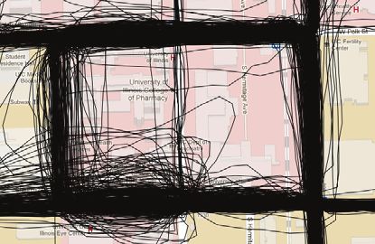
precision + recall (1 − spurious) + (1 − missing) For trace data, 118 h of GPS traces from the University of Illinois at
Chicago campus shuttles were used. In addition to traveling around
The higher the F-score, the closer the match. Sampling the maps campus, these shuttles pass through two different areas that contain
locally is an important aspect of this approach as it provides the abil- relatively tall buildings and significant GPS error. Figure 5a provides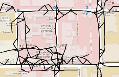
(a)                                                               (b)

                            (c)                                                               (d)

                            (e)                                                               (f)

                            (g)                                                               (h)

FIGURE 5   Raw data and results from three implemented algorithms in areas with high and low GPS error: (a) raw data,
high-error sample; (b) raw data, low-error sample; (c) Davies algorithm, high-error sample; (d) Davies algorithm, low-error
sample; (e) Cao algorithm, high-error sample; (f) Cao algorithm, low-error sample; (g) Edelkamp algorithm, high-error sample;
and (h) Edelkamp algorithm, low-error sample.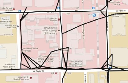
68 Transportation Research Record 2291
an example of the distribution of the traces and GPS errors found in the Main Quantitative Results
study data set for one of these areas of high GPS error. In this evalua-
tion, the entire data set was studied, as was a subset of the data drawn Figure 6 shows the main results and shows the performance of the
from an area of low-rise buildings where there is very little GPS error three algorithms for a varying matching threshold. The matching
(see the sample in Figure 5b). Because GPS error can be a problem threshold is the allowable distance between a hole and a marble. A
for map inference algorithms, the partitioning of the data in this way detailed discussion of these results follows.
allows the performance of the algorithms to be tested and compared Figure 6a shows the performance of the three algorithms as tested
on both a realistic and a somewhat idealized data set. The road maps on the full data set. For small matching thresholds, the fine-grained
generated by each algorithm are depicted in Figure 5, c to h. spatial accuracy of the algorithm is significant. The Davies and Cao
algorithms both underperform the Edelkamp algorithm at a 5-m
matching threshold. For the Davies algorithm, this performance
Davies et al. (4) is explained by the fact that the algorithm generates a single, bi-
directional centerline, whereas the others produce one edge in each
Visually, the algorithm from Davies et al. produces superior maps direction. On a wide road, the distance between the centerline and
in areas with large GPS error. Because this method avoids treating the center of the road in one direction may well exceed 5 m. A simi-
GPS traces individually and, instead, uses them in aggregate to find lar problem is exhibited by the Cao algorithm, in which lanes in
the road boundaries, the method is able to create one road from a opposite directions are artificially spread apart to improve legibility.
large collection of relatively diverse traces. This aspect of the algo- This introduces a slight error, which shows up as a poor matching
rithm is illustrated in the difficult high-error case in Figure 5c, in performance for a 5-m threshold.
which the algorithm accurately extracted the road topology without In the low-error data set, all of the algorithms unsurprisingly
adding any extraneous edges. In the low-error case in Figure 5d, achieved a higher F-score (see Figure 6b). However, although the
the result is largely the same. However, note the absence of the
Davies algorithm continued to outperform the Edelkamp algorithm at
less-traveled road segment on the right. This absence illustrates the
15- and 25-m matching thresholds, the prevalence of wide, median-
fundamental trade-off of this algorithm: any given threshold value
separated two-way roads in this data set allowed the Edelkamp algo-
must compromise between introducing noise in high-density areas
rithm to outperform the Davies algorithm at both the 5- and 10-m
and losing infrequently traveled edges in low-density areas.
matching thresholds.
Cao and Krumm (5)
Addressing Directionality Finding
The clarification preprocessing step performed in the algorithm devel- in Davies et al. (4)
oped by Cao and Krumm helps to reduce GPS noise before the map
generation and, in noise-free areas, results in cleanly generated maps, In contrast with the other two approaches, the Davies algorithm
as demonstrated in Figure 5f. However, the clarification has its limits generates a single centerline for each street, with a directionality
in areas with high GPS error, in which spatially dispersed traces are annotation. As mentioned earlier, the authors in Davies et al. use
unable to become tightly banded. As a result, when the trace-merging a technique that measures the direction of travel through each grid
method is applied to the clarified data, residual noise results in the cell to extract the permitted directions of travel. However, in the
spurious roads seen in Figure 5e. Although this algorithm attempts to testing described in this paper, this method did not fare well. Many
prune spurious roads after map generation, its efforts are largely futile streets that were bidirectional in the ground truth were not repre-
in areas of high GPS noise in which edge volume is widely distributed. sented as such in the inferred map. To correct for this problem, two
different modifications to the Davies algorithm were made.
First, the direction-finding component of the Davies algorithm
Edelkamp and Schrödl (3) was discarded, making every road bidirectional. Although this mod-
ification allowed bidirectional roads whose directionality had been
The algorithm in Edelkamp and Schrödl creates road segments by
incorrectly inferred to be correctly represented, the modification
joining clusters based on the underlying trace data and works well
also introduced the problem of incorrectly representing one-way
in areas with low GPS noise, as can be seen in Figure 5h. However,
this cluster-joining method is easily led astray by GPS noise and streets as bidirectional. On the full data set, which included a large
results in spurious roads being produced, as illustrated in Figure 5g. number of one-way streets, this trade-off resulted in a performance
Because this algorithm does not attempt to prune spurious roads decrease, as can be seen in Figure 6c. In the low-error data set,
after generation, all of these roads remain in the final road map. however, which consisted predominantly of bidirectional roads, the
However, the implementation described here does not include inter- bidirectional Davies implementation achieved a notable performance
section refinement and lane finding. These features would likely gain (see Figure 6d).
have improved the results on the low-error data set but would have As an alternative to the directionality-finding technique in
had little or no effect on the high-error data set. Davies et al. (4), the GPS traces were matched onto the inferred
bidirectional map through the use of Viterbi map matching (31).
The resulting sequences of road segments were then used to infer
Quantitative Evaluation road directionality. The relative performance of the three techniques
is shown in Figure 6, c and d. The line marked “Davies” is identical
In this section, the robust map comparison method described ear- to the one in Figure 6, a and b. On top of an already strong perfor-
lier is used to quantitatively evaluate the three representative algo- mance, this map-matching technique gives the KDE-based algo-
rithms described in the previous section. Parameter selection and rithm by Davies et al. a significant advantage over the a lternative
implementation are also discussed. approaches.Biagioni and Eriksson 69
(a) (b)
(c) (d)
(e) (f)
FIGURE 6 Results of algorithm analysis: (a) F-score, three algorithms, full data set; (b) F-score, three
algorithms, low-error data set; (c) F-score, three Davies algorithms, full data set; (d) F-score, three
Davies algorithms, low-error data set; (e) precision and recall, Davies map-matched algorithm, varying
density threshold, full data set; and (f) precision and recall, Davies map-matched algorithm, varying density
threshold, low-error data set.
Remaining Challenges Parameter Sensitivity and
Implementation Details
Some challenges remain, even with the map-matching improvements
made to the Davies algorithm. Primarily, the choice of a density Each of the algorithms described earlier includes several tuning
threshold for the Davies algorithm is made globally across the entire parameters. A sensitivity analysis was conducted to determine which
map. If the chosen threshold value is too low, excess noise is added of those parameters most significantly affect the performance by fixing
to the map in the form of spurious roads. If the value is too high, the values of one parameter and allowing all the others to vary. Some
portions of the map with relatively low density are treated as spuri- of the results of this analysis are discussed in the following sections.
ous and removed, resulting in missing roads. This behavior is illus-
trated in Figure 6, e and f. It can be seen that as the density threshold
increases, the proportion of spurious edges decreases (i.e., precision Implementation of Davies et al. (4)
increases), and the proportion of missing edges first decreases (i.e.,
recall increases) as excess noise is removed and then increases (i.e., The implementation of the Davies algorithm closely follows the
recall decreases) as low-density roads are pruned from the map. It description given in the paper by Davies et al. (4), with the addi-
is believed that this insight is the key to further improvements to the tional modifications discussed in the section on addressing direc-
KDE-based method: only marginal improvements will be made as tionality finding in the algorithm. The parameters for this algorithm
long as the constant threshold used in the current algorithm remains. are the cell size, the density threshold, the kernel bandwidth, and70 Transportation Research Record 2291
(a) (b)
(c) (d)
(e) (f)
FIGURE 7 Parameter sensitivity testing over several matching distance thresholds: (a) cell size parameter
(Davies map-matched algorithm), (b) density parameter (Davies map-matched algorithm, density threshold
5 number of traces per cell), (c) volume parameter (Cao algorithm, volume threshold 5 number of traces),
(d) number of traces used (Cao algorithm), (e) number of traces used (Edelkamp algorithm), and (f) distance
parameter (Edelkamp algorithm).
the number of traces used to generate the map. Figure 7, a and b, old and the number of traces used to generate the map. As shows in
show this algorithm’s sensitivity to cell size and density threshold. Figure 7c (threshold range 0–5), an increase in the edge volume thresh-
Figure 7a shows that a smaller cell size will always produce a better old, which is used to prune spurious edges from the generated map,
result with a fixed kernel bandwidth, as this simply improves gran- increases map accuracy, as spurious edges are removed. However,
ularity. Figure 7b shows that an increase in the density threshold if the pruning is too aggressive (i.e., the volume threshold is set too
increases accuracy as noise is removed from the map. However, this high), legitimate roads may end up being incorrectly removed, which
process will eventually lead to low-density roads being removed decreases the accuracy (as seen in Figure 7c, threshold range 5–50). In
from the map and result in a decrease in accuracy. Figure 7d, the performance decreases with the number of traces used to
generate the map; this is a result of the increased noise that comes with
a larger data set and this algorithm’s inability to overcome that error.
Implementation of Cao and Krumm (5)
The implementation of the Cao algorithm follows the description in Implementation of Edelkamp and Schrödl (3)
Cao and Krumm closely (5), with map generation being preceded by
clarification. The parameters for this algorithm are the edge volume The implementation of the Edelkamp algorithm follows the description
threshold, the location distance limit, the location bearing difference in Edelkamp and Schrödl (3), with the exception that no intersection
threshold, and the number of traces used to generate the map. Figure 7, refinement is performed. The parameters for this algorithm are the
c and d, show this algorithm’s sensitivity to the edge volume thresh- cluster seed interval, the intracluster bearing difference threshold,Biagioni and Eriksson 71
the intracluster distance threshold, and the number of traces used to 7. Niehoefer, B., R. Burda, C. Wietfeld, F. Bauer, and O. Lueert. GPS
generate the map. Figure 7, e and f, show this algorithm’s sensitiv- Community Map Generation for Enhanced Routing Methods Based on
Trace-Collection by Mobile Phones. Proc., 1st International Conference
ity to the number of traces and the intracluster distance threshold on Advances in Satellite and Space Communications, Colmar, France,
parameters. Figure 7e shows that performance decreases with the IEEE, New York, 2009, pp. 156–161.
number of traces used to generate the map, because, similarly to 8. Mitchell, T. Machine Learning, 1st ed. McGraw-Hill Education, New
the Cao algorithm, the larger data set includes more noise, which York, 1997.
this algorithm is unable to overcome. Also, Figure 7f data show that 9. Scott, D. W. Kernel Density Estimators. In Multivariate Density Esti-
mation: Theory, Practice, and Visualization, John Wiley & Sons, Inc.,
performance improves with increasing intracluster distance, as this Hoboken, N.J., 2008, pp. 125–193.
increases the clusters’ resistance to noise in the GPS traces. 10. Worrall, S., and E. Nebot. Automated Process for Generating Digitised
Maps Through GPS Data Compression. Proc., Australasian Conference
on Robotics and Automation, Brisbane, Australia, Australian Robotics
Algorithm Run Time and Automation Association, Sydney, Australia, 2007.
11. Guo, T., K. Iwamura, and M. Koga. Towards High Accuracy Road
The run time of these algorithms varies dramatically as a result of Maps Generation from Massive GPS Trace Data. Proc., International
differences in algorithmic complexity. Particularly, the Cao algorithm Geoscience and Remote Sensing Symposium, Barcelona, Spain, IEEE,
New York, 2007, pp. 667–670.
suffers in dense neighborhoods, in which it exhibits quadratic com- 12. Chen, C., and Y. Cheng. Roads Digital Map Generation with Multi-Track
plexity. On a subset of 100 traces, the Cao algorithm finished in 2.5 h, GPS Data. Proc., International Workshop on Education Technology and
the Edelkamp algorithm in 73 s, and the Davies algorithm in 8 s. Training and International Workshop on Geoscience and Remote Sensing,
The map-matched version of the Davies algorithm finished in 106 s. Shanghai, China, Vol. 1, IEEE, New York, 2008, pp. 508–511.
13. Shi, W., S. Shen, and Y. Liu. Automatic Generation of Road Network
On the full set of 899 traces, the Cao algorithm required 2.5 days, the Map from Massive GPS, Vehicle Trajectories. Proc., Conference on
Edelkamp algorithm 15 min, and the Davies algorithm 25 s. The 12th International Intelligent Transportation Systems, St. Louis, Mo.,
map-matched version of the Davies algorithm finished in 14 min. IEEE, New York, 2009, pp. 1–6.
14. Jang, S., T. Kim, and E. Lee. Map Generation System with Lightweight
GPS Trace Data. Proc., 12th International Conference on Advanced
Conclusion Communication Technology, Gangwon-Do, South Korea, Vol. 2, IEEE,
New York, 2010, pp. 1489–1493.
Robust quantitative evaluation methods and a rigorous comparison 15. Naver. http://dev.naver.com/openapi/apis/map/. Accessed Nov. 14, 2011.
16. Piegl, L., and W. Tiller. The NURBS Book, 2nd ed. Springer-Verlag,
with prior work are important tools for furthering any field of scien- New York, 1997.
tific inquiry. With the new tools presented here, three algorithms from 17. NAVTEQ Maps and Traffic. http://www.navteq.com/. Accessed July 22,
the literature were compared. Overall, the algorithm by Davies et al. 2011.
(4) was found to significantly outperform the others under a variety 18. Wong, S. S. M. Computational Methods in Physics and Engineering.
World Scientific, Singapore, 1997.
of conditions. Through the quantitative evaluation method presented
19. Hastie, T., and W. Stuetzle. Principal Curves. Technical report 151.
in this paper, opportunities for further improvement to this algorithm University of Washington, Seattle, 1988.
were identified. Some of these improvements were implemented and 20. Agamennoni, G., J. I. Nieto, and E. M. Nebot. Technical report: Inference
evaluated here and yielded a further, significant performance improve- of Principal Road Paths Using GPS Data. Technical report. Australian
ment. The new tools offered in this paper are expected to help bring Centre for Field Robotics, University of Sydney, Australia, 2010.
http://www-personal.acfr.usyd.edu.au/jnieto/Research-files/
significant advances to the study of map inference from GPS traces. PRPInferenceReport2010.
21. Khanna, M. Introduction to Particle Physics. Prentice-Hall, New Delhi,
India, 2004.
Acknowledgments 22. Hastie, T., R. Tibshirani, and J. Friedman. The Elements of Statistical
Learning: Data Mining, Inference, and Prediction. Springer, New York,
This material is based on work supported by the National Science 2009.
Foundation, as well as by the Transportation Research Board of 23. Leler, W. J. Human Vision, Anti-Aliasing, and the Cheap 4000 Line
the National Academies through Transit Innovations Deserv- Display. Proc., 7th Annual Conference on Computer Graphics and
Interactive Techniques, Seattle, Wash., Association for Computing
ing Exploratory Analysis Project-65: A Context-Aware Transit Machinery, New York, 1980, pp. 308–313.
Navigator. 24. Yokoi, S., J. Toriwaki, and T. Fukumura. An Analysis of Topological
Properties of Digitized Binary Pictures Using Local Features. Computer
Graphics and Image Processing, Vol. 4, No. 1, 1975, pp. 63–73.
References 25. Aurenhammer, F. Voronoi Diagrams—A Survey of a Fundamental Geo-
metric Data Structure. ACM Computing Surveys, Vol. 23, No. 3, 1991,
1. Agamennoni, G., J. Nieto, and E. Nebot. Robust Inference of Principal pp. 345–405.
Road Paths for Intelligent Transportation Systems. IEEE Transactions 26. Conte, D., P. Foggia, C. Sansone, and M. Vento. Thirty Years of Graph
on Intelligent Transportation Systems, Vol. 12, No. 1, 2011, pp. 298–308. Matching in Pattern Recognition. International Journal of Pattern
2. BITS Networked Systems Laboratory. http://bits.cs.uic.edu/. Accessed Recognition & Artificial Intelligence, Vol. 18, No. 3, 2004, pp. 265–298.
July 22, 2011. 27. Cormen, T. Introduction to Algorithms. MIT Press, Cambridge, Mass.,
3. Edelkamp, S., and S. Schrödl. Route Planning and Map Inference 2001.
with Global Positioning Traces. In Computer Science in Perspective 28. Bunke, H. On a Relation Between Graph Edit Distance and Maximum
(R. Klein, H.-W. Six, and L. Wegner, eds.), Vol. 2598 of Lecture Notes Common Subgraph. Pattern Recognition Letters, Vol. 18, No. 8, 1997,
in Computer Science, Springer, Berlin, 2003, pp. 128–151. pp. 689–694.
4. Davies, J. J., A. R. Beresford, and A. Hopper. Scalable, Distributed, 29. Liu, B. Web Data Mining: Exploring Hyperlinks, Contents, and Usage
Real-Time Map Generation. IEEE Pervasive Computing, Vol. 5, No. 4, Data. Springer, New York, 2007.
2006, pp. 47–54. 30. OpenStreetMap. http://www.openstreetmap.org/. Accessed July 22, 2011.
5. Cao, L., and J. Krumm. From GPS Traces to a Routable Road Map. 31. Thiagarajan, A., L. Sivalingam, K. LaCurts, S. Toledo, J. Eriksson, S.
Proc., 17th ACM SIGSPATIAL International Conference on Advances Madden, and H. Balakrishnan. Proc., 7th ACM Conference on Embedded
in Geographic Information Systems, Seattle, Wash., Association for Networked Sensor Systems, Berkeley, Calif., Association for Computing
Computing Machinery, New York, 2009, pp. 3–12. Machinery, New York, 2009, pp. 85–98.
6. Schroedl, S., K. Wagstaff, S. Rogers, P. Langley, and C. Wilson. Mining
GPS Traces for Map Refinement. Data Mining and Knowledge Discovery, The Geographic Information Science and Applications Committee peer-reviewed
Vol. 9, No. 1, 2004, pp. 59–87. this paper.You can also read