A Novel Automatic Modulation Classification Method Using Attention Mechanism and Hybrid Parallel Neural Network - MDPI
←
→
Page content transcription
If your browser does not render page correctly, please read the page content below
applied
              sciences
Article
A Novel Automatic Modulation Classification Method Using
Attention Mechanism and Hybrid Parallel Neural Network
Rui Zhang *, Zhendong Yin *, Zhilu Wu and Siyang Zhou

                                          Electronics and Information Engineering, Harbin Institute of Technology, Harbin 150001, China;
                                          wuzhilu@hit.edu.cn (Z.W.); zhousiyang@stu.hit.edu.cn (S.Z.)
                                          * Correspondence: 17B905026@stu.hit.edu.cn (R.Z.); yinzhendong@hit.edu.cn (Z.Y.)

                                          Abstract: Automatic Modulation Classification (AMC) is of paramount importance in wireless
                                          communication systems. Existing methods usually adopt a single category of neural network
                                          or stack different categories of networks in series, and rarely extract different types of features
                                          simultaneously in a proper way. When it comes to the output layer, softmax function is applied
                                          for classification to expand the inter-class distance. In this paper, we propose a hybrid parallel
                                          network for the AMC problem. Our proposed method designs a hybrid parallel structure which
                                          utilizes Convolution Neural Network (CNN) and Gate Rate Unit (GRU) to extract spatial features
                                          and temporal features respectively. Instead of superposing these two categories of features directly,
                                          three different attention mechanisms are applied to assign weights for different types of features.
                                          Finally, a cosine similarity metric named Additive Margin softmax function, which can expand the
                                          inter-class distance and compress the intra-class distance simultaneously, is adopted for output.
                                          Simulation results demonstrate that the proposed method can achieve remarkable performance on
                                an open access dataset.


Citation: Zhang, R.; Yin, Z.; Wu, Z.;     Keywords: Automatic Modulation Classification; attention mechanism; Convolution Neural Net-
Zhou, S. A Novel Automatic                work; gate recurrent unit; AM-Softmax; deep learning
Modulation Classification Method
Using Attention Mechanism and
Hybrid Parallel Neural Network.
Appl. Sci. 2021, 11, 1327. https://       1. Introduction
doi.org/10.3390/app11031327
                                                Automatic Modulation Classification (AMC) is an intermediate step between signal
                                          detection and demodulation. The aim of AMC is to identify the modulation type of re-
Academic Editor: Bo Wei and
                                          ceived signal correctly and automatically, which reveals a broad application foreground
Wai Lok Woo
                                          both in civil and military technologies [1]. In civilian aspects, AMC can be applied to
Received: 29 December 2020
Accepted: 29 January 2021
                                          ensure the normal communication of legitimate users by monitoring legitimate spectrum
Published: 2 February 2021
                                          and identifying illegitimate interference. AMC can also be used to reinforce and foster
                                          situational awareness in soft-defined radio system for better spectrum utilization [2]. In a
Publisher’s Note: MDPI stays neutral
                                          non-orthogonal multiple access system, AMC can identify the modulation type of non-
with regard to jurisdictional claims in
                                          orthogonal multiple access system and decide whether successive interference cancellation
published maps and institutional affil-   is required or not [3]. In military aspects, AMC is the core technology of electronic counter-
iations.                                  measures, communication surveillance and jamming. AMC can help intercept receivers
                                          to get the correct modulation type, which provides a reference basis for demodulation
                                          algorithm selection of demodulator and is helpful to the selection of optimal jamming
                                          pattern or jamming cancellation algorithm for electronic warfare, so as to ensure friendly
Copyright: © 2021 by the authors.
                                          communication and suppress and destroy enemy communication, so as to achieve the
Licensee MDPI, Basel, Switzerland.
                                          purpose of electronic warfare communication countermeasure [4]. Consequently, it is
This article is an open access article
                                          absolutely imperative to develop AMC technology.
distributed under the terms and                 Extant literature can be divided into two categories: maximum likelihood-based and
conditions of the Creative Commons        feature-based approaches. Maximum likelihood-based approaches can be divided into 3 cat-
Attribution (CC BY) license (https://     egories: average likelihood ratio test (ALRT) [5], generalised likelihood ratio test (GLRT) [6]
creativecommons.org/licenses/by/          and hybrid likelihood ratio test (HLRT) [7]. For maximum likelihood-based approaches,
4.0/).                                    AMC problems can be reviewed as a hypothesis testing problem. Specifically, according to

Appl. Sci. 2021, 11, 1327. https://doi.org/10.3390/app11031327                                               https://www.mdpi.com/journal/applsci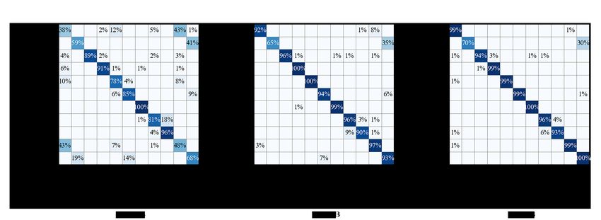
Appl. Sci. 2021, 11, 1327                                                                                                  2 of 19

                            the statistical characteristics of the signal, different statistics for classification are calculated,
                            and then compared with an appropriate threshold to form a decision rule. The most popular
                            statistics are average likelihood radio, generalised likelihood ratio and hybrid likelihood
                            ratio. Maximum likelihood-based approaches can get the optimal solutions theoretically,
                            but they suffer from high computational complexity and require much prior information.
                            These shortcomings greatly restrict their application. In contrast, feature-based approaches
                            can achieve suboptimal solutions with much lower computational complexity and less prior
                            information, which make feature-based approaches more practical.
                                  Feature-based approaches can be divided into traditional AMC methods and deep
                            learning methods. The features traditional AMC methods ultilized are handcraft features
                            and the classifiers usually choose traditional machine learning methods such as support
                            vector machine [8], decision tree [9] and K-neighbourhood algorithms [10]. The most popu-
                            lar handcraft features are High-Order Cumulant features [11], cyclic spectrum features [12]
                            and Wigner Ville distribution features [13]. Whereafter, different machine learning methods
                            are used for classification. There are also some non-machine learning methods for AMC.
                            Alharbi [14] pre-computed thresholds for AMC in the presence of high frequency noise.
                            Jagannath [15] calculated thresholds for inter-class recognition and applied expectation-
                            maximization method for intra-class recognition. However, handcraft features only show
                            characteristics of one specific domain and simple threshold methods cannot handle com-
                            plex situations. If we need more accurate description of signal, we have to select different
                            types of handcraft features and concatenate them for classification [16]. However, when
                            facing lower Signal to Noise Ratio (SNR) and more modulation types, handcraft features
                            are not enough for classification. Thus, we need more powerful AMC algorithms.
                                  The proliferation of deep learning has recently leaped into the modulation classi-
                            fication. Deep learning has been proposed in [17], which proposed deep Convolution
                            Neural Network (CNN). Deep learning has developed rapidly and widely been applied
                            in computer vision [18], speech recognition [19], natural language processing [20], etc.
                            While widely applied in various domains, deep learning has also grown tremendously.
                            In addition to CNN, Long Short-Term Memory (LSTM) network [21], Residual Neural
                            Network (ResNet) [22] and many other deep learning structures are developed for different
                            problems. Deep neural networks put feature extraction and classifier construction together,
                            they are trained simultaneously. Deep neural networks are trained automatically to find the
                            most suitable features and the corresponding classifier for the input dataset; hence, deep
                            learning algorithms can obtain more expressive features than handcraft features. Therefore,
                            deep neural networks have been more and more popular in AMC domain.
                                   Deep learning methods consist of two categories depending on the input of neural
                            networks is raw data or not. The input of Feed-forwards neural network (FNN) and CNN
                            can be features extracted from traditional machine learning methods. Ref. [23] calculated
                            amplitude variance, maximum value of the power spectral density of the normalized centered-
                            instantaneous amplitude, in-band spectral variation, high order statistics and deviation from
                            unit circle as input features, the classifier is a designed artificial neural network. Ref. [24]
                            extracted High-Order Cumulant features, the standard deviation of the absolute value of the
                            non-linear component of the instantaneous phase and the peak to average radio as features,
                            the classifier is a designed 4-layer artificial neural network. Ref. [24] can recognize modulation
                            types under fading channels. Some literatures mapped the input IQ signal to some types of
                            images, and then trained them by CNN designed from computer vision domain. Ref. [25]
                            mapped the IQ signal to constellation images and applied AlexNet and GoogleNet from
                            computer vision domain for classification. Ref. [26] mapped the input signal to ambiguity
                            function images and utilized stacked sparse auto-encoder to extract features, the classifier is a
                            two-layer neural network. Ref. [27] transformed very high frequency radio signals to cyclic
                            spectrum images and classified by CNN and the accuarcy reached 95% for an SNR or 2 dB.
                            However, transformations of the raw signal will Inevitably result in a part of information loss
                            and the deep learning methods have ability to handle raw signals. Thus, the second category
                            is to process the raw data directly.
Appl. Sci. 2021, 11, 1327                                                                                          3 of 19

                                   O’shea [28] first provided the standard dataset and the baseline network of AMC.
                            Deep Belief Network [29] has been applied in AMC early but shown lower accuracy than
                            conventional discriminant model. Rajendran [30] projected the amplitude and phase of each
                            samples and put the transformed signal into a 2-layer LSTM network for classification and
                            exceeded more than 80% accuracy for an SNR of 10 dB under O’shea’s dataset. Ref. [31]
                            applied GRU for AMC with resource-constrained end-devices. Utrilla [32] designed a LSTM-
                            based denoising autoencoder classifier and exceeded 90% for an SNR of 4 dB. West [33]
                            utilized Inception structure [34] and Residual module to extract features and can reach
                            80% accuracy for an SNR of 0 dB. Liu [35] proposed a Convolutional Long Short-term
                            Deep Neural Network (CLDNN) which cascaded CNN and LSTM. Hermawan [36] pro-
                            posed an CNN-based method adding Gaussian noise layer and performed better than
                            baseline. Dropout-replaced Convolutional Neural Network (DrCNN) [37] was proposed
                            which replaced max pooling layer with dropout layer [38] and obtain a competitive result.
                            Huang [39] combined ResNet and GRU and reached 95% for an SNR of 5 dB. Tao [40]
                            proposed sequential convolutional recurrent neural network which connected CNN and
                            bi-LSTM in series and got a competitive result. However, serial structure of CNN and
                            RNN aliases different types of features, which will result in the loss of information in-
                            evitably. Thus, parallel structure with a proper feature combination method can reach a
                            better performance.
                                  Attention mechanism was proposed in 2017 [41], which has brought widespread at-
                            tention. Attention mechanism reweights the input features in order to highlight important
                            parts and suppress unimportant parts, which has widely used in natural language process-
                            ing [42], computer vision [43], and also aroused AMC’s interest, Yang [44] combined atten-
                            tion mechanism and one-dimension convolution module to propose an One-Dimensional
                            Deep Attention Convolution Network (OADCN) network for different modulation types
                            with different channel coding mode. Nevertheless, attention mechansim is only applied to
                            assign weights for spatial features from CNN model, it still has broad application prospects.
                                  Softmax function [45] is the most popular classification function in AMC. Softmax
                            function can amplify the difference between outputs. However, there are also many output
                            functions for neural network. Cosine-similarity-based function has become popular re-
                            cently [46]. Existing literature rarely considers cosine-similarity distance for AMC problem.
                            As a consequence, this paper proposed the idea of applying cosine similarity softmax called
                            Additive margin softmax (AM-softmax) [47] which is widely utilized in metric learning to
                            AMC problem.
                                  In this paper, we propose a hybrid parallel module which concatenates spatial fea-
                            tures and temporal features simultaneously, utilizing attention mechanism to reweight all
                            features. At first, a hybrid parallel feature extraction module is designed for extracting
                            features in parallel. CNN and GRU are applied to extract spatial features and temporal
                            features, respectively. Then the two types of features are concatenated in the channel
                            dimension. Different attention mechanisms are applied to assign weights for features.
                            Squeeze-and-Excitation (SE) block and multi-head attention mechanism are put into use
                            for assigning weights for features in channel dimension and feature dimension respectively.
                            The iterative Attentional Feature Fusion (iAFF) module is utilized for weights assignment
                            in the residual shortcut structure. We use SE block and multi-head attention mechanism
                            to construct hybrid parallel feature extraction module and build a residual structure with
                            hybrid parallel feature extraction module and iAFF module. Finally, we flatten the output
                            features, apply multi-head attention mechanism to each point in features, and send the
                            features to AM-softmax to calculate the cosine-similarity distance. To our knowledge, this
                            is the first paper utilizing cosine similarity softmax in the AMC domain.
                                  The remainder of the paper is organized as follows: In Section 2, we will show the
                            details of our proposed method. In Section 3, we evaluate the performance of the proposed
                            model with simulation results. Finally, we summarize the content of this paper in Section 4.
Appl. Sci. 2021, 11, 1327 4 of 19
2. Methods
2.1. System Model
The system model of our method is shown as Figure 1, the first module is prepro-
cessing module. x IQ is the input data of our model. The input data is IQ representation.
The real part and the imaginary part of the input signal consist of 2 channels. We first
calculate the amplitude and phase features of the IQ signal. We next concatenated the raw
complex data with these two features and got dataset with 4 channels. The purpose of
this concatenation is to achieve data augmentation. The detail of this operation will be
shown in Section 3.2. After preprocessing module, the concatenated data is sent to the
classification module, which is achieved by our proposed hybrid parallel network. The
output of our network is the classification result.
Figure 1. The system model of our proposed method.
2.2. Hybrid Parallel Network
The hybrid parallel network is stacked by the hybrid parallel module we proposed.
The hybrid parallel module combines Inception, Gate Recurrent Unit (GRU), Squeeze-and-
Excitation (SE) block, iterative Attentional Feature Fusion (iAFF) module and a multi-head
attention mechanism. The output function is an Addictive Margin (AM)-Softmax function.
We will first show the whole structure and then introduce each module in sequence.
Figure 2 is the structure of the proposed hybrid parallel network. The hybrid parallel
network is composed of several hybrid parallel modules. The core structure of the hybrid
parallel module is the hybrid parallel feature extraction module. Figure 2a illustrates the
hybrid parallel feature extraction module. The parallel structure is constructed by Inception
and GRU. The inception module and GRU module aim to extract spatial features and
temporal features, respectively. The SE block adjusts the weight of each channel. Before the
Inception module we normalize the features by Batch Normalization (BN ). The Maxpool
layer is applied when the stride of Inception is greater than 1, the length of Maxpool is
equal to the stride of Inception. After obtaining spatial features and GRU features, we
normalize and reweight the splicing features by multi-head attention mechanism. Our
proposed hybrid parallel module combines the parallel feature extraction module and
iAFF module. The short skip to the iAFF module is a convolution module with the 1 × 1
kernel in order to adjust the channel size of the initial input. The hybrid parallel network
is presented on Figure 2b. We stack several hybrid parallel modules by residual structure
to extract temporal and spatial features. After the last hybrid parallel module, we flatten
all the features and readjust the weight of each sample point by multi-head attention
mechanism. Finally, we output the result through AM-softmax function. The details of all
the constructed modules are shown in the following sections.Appl. Sci. 2021, 11, 1327 5 of 19
Figure 2. The structure of the hybrid parallel network (a) The parallel feature extraction module
which is the basic component of the hybrid parallel module. (b) The structure of the hybrid parallel
network which is composed of several the hybrid parallel modules.
2.3. CNN and GRU Module
2.3.1. Convolution Neural Network (CNN)
Convolution neural network was first proposed in [17] for imageNet competition
and reached the first immediately. CNN has more powerful data processing abilities than
traditional full-connected neural network. CNN can preserve the neighborhood relations
and spatial locality of input data at feature representation [48]. As long as the input data
is enough, the CNN model can train itself automatically. The CNN structure is entirely
derived from the training data, thus the network is fully adapted to the data and can obtain
more representative features. The core idea of CNN is the convolution step, which can
be viewed as a correlated process. Assuming that ω1 , ω2 , . . . , ωm represent the weight of
1-D convolution kernel of length m, the computational process of 1-D convolution can be
represented as:
m
y t = f ( ∑ ω k · x t − k +1 ), (1)
k =1
where xt is the input sample at time t, yt is the superposition of the information generated
at the current moment t and the information delayed at the previous moment, f (·) is the
activation function. The activation function we choose in this paper is Rectified Linear Unit
(ReLU) [49], which can be defined as:
(
x, x > 0,
ReLU ( x ) = (2)
0, x ≤ 0
In this paper, we choose ReLU as our activation function after 1-D convolution pro-
cessing. The typical way to increase capacity for CNN is to go deeper and wider on
structure. Going deeper means stacking more layers, going wider needs more channels,
both methods will increase the computational overhead. Inception [34] was proposed to
solve this problem. The structure of Inception module applied in this paper is shown as
Figure 3:Appl. Sci. 2021, 11, 1327 6 of 19
Figure 3. The structure of Inception block used in this paper.
The module 1 × 1 Kernel means that the kernel size of 1-D convolution process is 1 × 1.
Similarly, 1 × 3, 1 × 5, 1 × 7 represent the convolution kernel size as 1 × 3, 1 × 5 and 1 × 7
respectively. After performing convolution operations, Inception module concatenates all
output at channel dimension. Different scale of kernel size can help Inception to extract
different features in different spatial scale. The next step of inception is Batch Normalization
(BN ) [50]. The BN layer accelerates training by normalizing features at one batch:
Nbatch
1
µ=
Nbatch ∑ xn ,
n =1
Nbatch
1
σ2 =
Nbatch ∑ ( x n − µ )2 , (3)
n =1
xn − µ
x̂ = √ ,
σ2 + ε
yn = γ xˆn + β,
where Nbatch denotes batch size, xn denotes the input data, µ and σ2 denote the mean and
variance of the batch, x̂ denotes the normalized data and ε is a constant to prevent zero gradient,
γ and β are learnable parameter vectors for fixing data, yn is the fixed output feature.
2.3.2. Gate Recurrent Unit (GRU)
Gate Recurrent Unit (GRU), a type of RNN, is proposed to solve the vanishing gradient
problem in back propagation of RNN. Compared to LSTM, GRU can reach the same
accuracy with cheaper computational cost. The forward propagation of GRU can be
denoted as:
rt = σLir ( xt ) + Lhr (ht−1 ),
zt = σLiz ( xt ) + Lhz (ht−1 ),
(4)
nt = tanh( Lin xt + rt ∗ Lhn (ht−1 )),
h t = (1 − z t ) ∗ n t + z t ∗ h t −1 ,
where xt is the input data at the time t, ht−1 is the hidden state at the last time, rt and zt
denote the reset gate state and the update gate state respectively, σ (·) denotes the sigmoid
function which is defined as
1
σ( x) = , (5)
1 + e− xAppl. Sci. 2021, 11, 1327 7 of 19
tanh(·) function is defined as
e x − e− x
tanh( x ) = , (6)
e x + e− x
L(·) denotes a full-connect layer which can be defined as:
Li ( x ) = Wi x + bi , (7)
Wi and bi are denoted as weight and bias respectively.
2.4. Attention Mechanism
Attention mechanism has a huge improvement effect on deep learning tasks. When
human beings are observing something seriously, they will definitely focus on what needs to
be observed and ignore the surrounding environment. This can be interpreted as human
beings assigning more weight to immediate things and less weight to the surrounding
environment. Attention mechanism is based on this principle by training itself to learn the
reweighting mechanism. Attention mechanism is able to pay more attention to the part
of the input which better express the characteristics of the signal. We choose three types
of attention mechanism called Squeeze-and-Excitation (SE) block [51], iterative Attention
Feature Fusion (iAFF) module [52] and Multi-head attention [41] for our model. SE block
focuses on channel-dimension weight distribution and is applied together with Inception for
spatial feature extraction. The iAFF module is applied for feature fusion from the same-layer
scenario to cross-layer scenarios which is called residual structure. iAFF module is placed
between two hybrid parallel modules to distribute features consist of inception module,
GRU module and the initial input. The multi-head attention module reweights all flattened
features before classification. The following sections will introduce these three attention
modules.
2.4.1. Squeeze-and-Excitation (SE) Block
The core idea of SE block is to assign weights to each channel. SE block has two
steps: squeeze step and excitation step. Squeeze step splits features in channel dimension.
SE block applies global average pooling in channel dimension and gets the channel-wise
statistics, the i-th element of the output z can be shown as:
D
1
zi =
D ∑ xi (8)
i =1
where xi is the i-th element of the input and z is a C-dimension vector. Then the output
vector is sent into a gating mechanism:
s = F ex (z, W ) = σ ( g(z, W )) = σ (W 2 δ(W 1 z)), (9)
C C
δ is defined as ReLU function, W 1 ∈ RC× r and W 2 ∈ R r ×C , they are both trainable
parameters and r is a hyper parameter called reduction ratio, controlling the bottleneck
of two full-connect layers with a non-linearity function ReLU. Finally, the weight of each
channel is rescaled by
x̄c = F scale ( xc , sc ) = sc xc , (10)
where x̄c is the c-th element of the output feature with dimension C × H, C is the number
of channel, H is the dimension of input feature. sc is the weight of c-th channel, xc refers to
the c-th input feature and F scale means channel-wise multiplication.
2.4.2. Iterative Attentional Feature Fusion (iAFF) module
Existing attention-based methods only focus on the features in the same layer, iAFF
module [52] can integrate cross layer features, making the fusion scheme more heuristicAppl. Sci. 2021, 11, 1327 8 of 19
and fuse the receive features in a contextual scale-aware way. The structure of iAFF is
shown as Figure 4:
Figure 4. The structure of the iterative Attentional Feature Fusion (iAFF) module. (a) The core
component of iAFF module called Multi-scale Attention Mechanism (MS-CAM). (b) The structure of
iAFF module.
Figure 4a is the core component of iAFF called Multi-scale Attention Mechanism(MS-
CAM), which aggregates local feature and global features via channel-dimension attention
and point-wise convolution. The input of MS-CAM is an intermediate feature X ∈ RC× H
with C channels and H-dimension features in one channel, the local channel context L( X )
is designed as
L( X ) = BN ( PWConv2 (δ(BN ( PWConv1 ( X ))))) (11)
where PWConv denotes point-wise convolution, BN denotes batch normalization. δ
denotes ReLU function. We define g ( X ) as global average pooling(Global Avg Pooling)
that can computed as
1 H
H∑
g (X ) = Xi (12)
i
PWConv1 has Cr channels and PWConv2 has C channels, PWConv1 and PWConv2 construct
a convolution bottleneck. The left part of MS-CAM can be seen as global channel feature
0
extraction and the right part is local channel feature extraction. The output feature X is
defined as
0
X = X ⊗ M ( X ) = X ⊗ δ( L( X ) ⊕ g ( X )) (13)
where ⊗ is the element-wise multiplication and ⊕ means broadcasting addition. M ( X ) is
the sum of global channel extracted features and local channel extracted features. iAFF
module in Figure 4b can be expressed as
X ] Y = M ( X + Y ) ⊗ X + (1 − M ( X + Y )) ⊗ Y,
(14)
Z = M (X ] Y ) Y + (1 − M ( X + Y )) Y,
Z denotes the output feature, Y can be output features of the interlayer. In this paper, Y is
the input of residual input. The dotted arrow from MS-CAM means 1 − M (·). The iAFF
module can be separated into two parts. The first part is X ] Y, the second part takes X ] Y
as the input of the next MS-CAM, and assigns its output as weight to X and Y.Appl. Sci. 2021, 11, 1327 9 of 19
2.4.3. Multi-Head Attention Mechanism
Attention mechanism divides features into multiple heads to form multiple subspaces,
allowing the model to pay attention to different aspects of feature information. We call
this practice the multi-head attention mechanism. The core idea of attention mechanism
is the scale dot-product attention mechanism. Q, K, V represent query, key and value,
respectively. In multi-head attention mechanism, they are all established by sending the
input to full-connect layer. Q and K have the same dimension dk ; thus, the output of scaled
dot-product Attention can be written as
QK T
Attention( Q, K, V ) = so f tmax ( √ )V (15)
dk
In this equation, K T means the transpose of K, the output vector is the reweighted
value V, the weight assigned to each value is calculated by K and Q. the dimension of Q, K
and V can be uniformly written as C × E, where C is the channel dimension and E denotes
embedding dimension. Q and K must have the same embedding dimension while the
embedding dimension of V can be different. The multi-head mechanism divides Q, K and
V into h parts, undertakes scaled dot-product attention h times and finally concatenates all
h outputs, which can be denoted by
MultiHead( Q, K, V ) = Concat(head1 , head2 , · · · , headh )W o ,
(16)
whereheadi = Attention( QWiQ , KWiK , VWiV ).
where W means the parameter matric. WiQ ∈ Rdmodel ×dk , WiK ∈ Rdmodel ×dk , WiV ∈ Rdmodel ×dv
and WiO ∈ Rhdv ×dmodel
2.5. Addictive Margin (AM)-Softmax Function
Softmax function is the most popular output function in classification task. Softmax
function is suitable in optimizing inter-class difference. However, If we can reduce intra-
class distance, we will also expand inter-class distance, and this will help to increase
classification accuracy. Cosine-similarity-based softmax aims to compute the angle between
the input vector and the center vector of modulation category. The process of narrowing
the angles within a class is also the process of widening the distance between classes.
Therefore, we choose cosine-similarity-based function for our modulation classification.
The softmax function can be written as
n WyT f i
1 e i
LS = −
n ∑ log WjT f i
,
i =1 ∑cj=1 e
(17)
1 n
ekWyi kk f i k cos(θyi )
=−
n ∑ log kWj kk f i k cos(θ j )
,
i =1 ∑cj=1 e
where f i is the i-th element of the output feature, Wj is the j-th column of the output.
The WyTi f i denotes the target score of the i-th sample. As is the equation shown, the softmax
function can be written as the product of the magnitudes of two vectors and the cosine
of their angular distance. As a result, the cos-similarity softmax can be implemented by
normalizing the weight vectors and the features. In this way, kWj k and k f i k are both
normalized to 1, and the data at the exponential position only leave the cosine of theAppl. Sci. 2021, 11, 1327 10 of 19
angular distance. Addictive Margin Softmax (AM-Softmax) is proposed to increase a cosine
margin in cos-similarity softmax, which is denoted as
1 n
es·(cos θyi −m)
L AMS = − ∑ log
n i =1 es·(cos θyi −m) + ∑cj=1,j6=yi es·cos θ j
n s·(WyT f i −m)
1 e i (18)
=−
n ∑ log s·(WyTi f i −m) sWjT f i
,
i =1 e + ∑cj=1,j6=yi e
wherekWj k = k f i k = 1,
s and m are both preset hyper parameters. m denotes the designed cos similarity margin
between classes. The difference between conventional softmax decision boundary and
AM-softmax decision boundary is shown in Figure 5.
Figure 5. Conventional Softmax’s decision boundary and Addictive Margin (AM)-softmax decision
boundary.
Where the red arrows W1 and W2 denote the center vectors of two modulation cate-
gories respectively. The decision boundary of conventional softmax function is the green
line P0 , where
cos(θW1 ,P0 ) = W1T P0 = W2T P0 = cos(θW2 ,P0 ). (19)
We must declare that the conventional softmax function in Figure 5 is not similar to
the softmax function applied in the existing literature. This is because W1 , W2 and P0 are all
normalized to 1 while the softmax function applied in existing literature do not normalize
parameters and features. Thus the conventional softmax function in Figure 5 is a type of
cosine similarity metrics. The decision boundary of softmax function bisects the angular of
two center vectors. For AM-softmax function, the decision boundary of the category W1
is at P1 . Similarly, the decision boundary of the category W2 is at P2 , the margin m can be
written as:
m = cos(θW1 ,P1 ) − cos(θW1 ,P2 ) = W1T P1 − W1T P2 (20)
The greater the value of m is, the larger the cosine similarity distance is. If m is set
to 0, that means the AM-softmax function degrades into a cosine-similarity metrics. s is
the scale parameter to accelerate convergence. If s is set too small, the convergence will
be too slow. However, if s is set too large, the convergence will be too fast to find better
local optimal value. Therefore, no matter the setting of m or the choice of s, the trainer
must be careful. In the training step, we widen the gap between the target logit and other
logits by at least m cosine margin. If the network is trained well, the output logit of the true
modulation category will be larger than others by a cosine value m in the test step. After
passing through the AM-Softmax function, the output will also be sent to a loss function
like cross entropy to optimize the performance of the network.Appl. Sci. 2021, 11, 1327 11 of 19
3. Results and Discussion
3.1. Dataset and Parameters
RML2016.10a [28] is the most popular dataset applied in AMC. RML2016.10a consists
of 11 modulation categories: BPSK, QPSK, 8PSK, 16QAM, 64QAM, BFSK, CPFSK, PAM4,
WB-FM, AM-SSB, and AM-DSB. Signal dimension is 2 × 128, the length of per sample is
128, each sample has real and imaginary parts, so the dataset has 2 channels. The duration
per sample is 128 µs. The sampling frequency is 1 MHz, the sampless per symbol is 8. The
number of samples under per SNR of each category is 1100, we choose 80% as our training
set, 10% as our validation set, 10% as our test set. The SNR range is from −20 dB to 18 dB,
but in practical applications, the communication conditions under −5 dB is useless for
communication, therefore we choose −4 dB to 18 dB for our experiments with interval of
2 dB. Therefore, the training samples in out experiments are 105,600, the validation samples
and test samples are both 13,200. The shape of our training set is 105, 600 × 2 × 128, the
shapes of validation set and the test set are both 13, 200 × 2 × 128.
The input of the whole network is the raw complex data concatenated with the cor-
responding amplitude and phase. The channel of the complex dataset is 2 including the
real data and its corresponding imaginary part. If we directly consider the two parts as two
channels, we will lose the relation between the real part and the imaginary part. Therefore,
we project the signal to polar coordinates and choose the amplitude and phase as two
channels to concatenate with the initial complex data, which can be written as
q
ai = reali 2 + imagi 2 ,
imagi (21)
pi = arctan
reali
where reali denotes the real part of the sample point and imagi denotes the imaginary of
the sample point ai and pi respectively denote the amplitude and phase the sample point.
Finally, we concatenate the amplitude channel and the phase channel with the complex
data, and the input data has 4 channels. The output of hybrid parallel network also needs
to be optimized by loss function. The loss function we choose is cross entropy, which is
defined as
K
L(l, y) = − ∑ tk log lk , (22)
k =1
where l is the output vector of AM-softmax, t denotes the label vector with one-hot formula-
tion, tk denotes the label of k-th element. Cross entropy loss can learn the difference between
two distribution and coverage fast; this is the reason why we choose cross entropy loss as
our loss function. The optimizer we choose is Adam optimizer [53], the initial learning rate
is set to 0.001 decayed by 10 every 16 epochs. The parameters of AM-Softmax we choose
are 0.1 for m and 10 for s. The batch size is set to 512 and we run 40 epochs for training.
Our proposed model cascades 4 hybrid parallel modules with different structure
parameters which is illustrated by the following table:
Table 1 illustrates the channels of the Inception modules applied in our structure. The
hidden size of corresponding GRU modules is all set to half of the channels of the second
Inception channels because of the bidirectional property. The size of the corresponding
channels of convolution modules and iAFF module is 2 times of the output channels
of Inception due to the concatenation of Inception and GRU. The number of multi-head
attention mechanisms in hybrid parallel modules is 4. The stride of the convolution module
in residual skip is 7 and the kernel size is 1 × 1. Following the last hybrid parallel module
we flat all the features and send it to a multi-head attention module with 10 heads. Before
the last AM-softmax function, we reduce the dimension of features by a linear layer with
the output size 128. The total parameters of our model are 27,415,424. After training, the
average inference time is 3 s.Appl. Sci. 2021, 11, 1327 12 of 19
Table 1. The structure of our proposed hybrid parallel network.
First Inception Channels Second Inception Channels Stride
64 40 1
40 80 2
40 40 2
20 20 1
3.2. Experiments and Discussion
We first explore the impact of the number of hybrid parallel modules. Figure 6
illustrates the performance of different hybrid parallel modules. We choose m = 0.1 and
s = 10. The average accuracy from one hybrid parallel module to 6 hybrid parallel modules
is 71.77%, 87.76%, 88.84%, 90.51%, 87.36% and 86.69%, respectively. We can find that only
one hybrid parallel module is not enough to learn the distribution of dataset. However,
when the number of modules is larger than 4, the performance of network is also not ideal.
This can be explained by too few modules not being enough to learn the distribution of
dataset. Nevertheless, too many modules will make back propogation difficult, which will
result in the problem of network degradation. As a result, our proposed method needs a
proper number of modules. In Figure 6, we find that the best number is 4.
Figure 6. The performance of different number of hybrid parallel modules.
The recognition rate of each modulation category for different SNRs is shown on
Figure 7. The network we applied stacks with 4 hybrid parallel module and sets m = 0.1
and s = 10, the average accuracy is 90.42%. We find that AM-DSB has always been
misclassifed a lot with WBFM. 8PSK is misclassified at first but the accuracy add up fast,
while at 0 dB, the accuracy surpasses 90%. Although the performance of some modulation
categories is not good at −4 dB, with the increase of SNR, the performance of all modulation
categories can exceed 95% except AM-DSB, which means that our proposed method has a
great performance on the digital-modulated signal and can also recognize some types of
analog modulation categories.Appl. Sci. 2021, 11, 1327 13 of 19
Figure 7. Classification accuracy of different modulation categories.
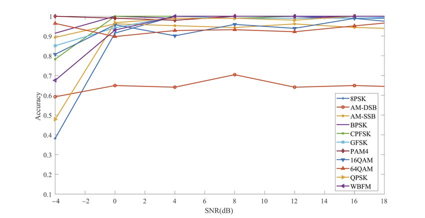
Next we analyze different confusion matrixs for an SNR of −4 dB, 0 dB and 6 dB. The
value −4 dB in Figure 8 is the lowest SNR so we can observe the confusion at low SNR.
When it comes to 0 dB, the SNR has increased and we can see the change in the confusion
matrix. The performance of our method becomes stable for an SNR of 6 dB. AM-DSB has
always been misclassified with WBFM, but WBFM can be successfully recognized. 16QAM
and 64QAM are misclassified for each other at −4 dB and the accuracy improves gradually
with the increase of SNR. This is owing to the fact that 16QAM and 64QAM both belong to
QAM modulation category. The same thing happens between 8PSK and QPSK. they are
misclassified with each other at −4 dB, and the accuracy reaches 99% at 6 dB. In summary,
the performance of digital-modulated signal is much better than analog-modulated signal.
We hold the opinion that this is because of two reasons: at the first, the number of analog-
modulated signal included in this dataset is less than digital-modulated signal. Secondly,
the distance between analog-modulated signal is shorter than the digital-modulated signal.
Figure 8. Confusion matrix of the hybrid parallel network for different Signal to Noise Ratios (SNRs). (a) The confusion
matrix of the hybrid parallel network for an SNR of −4 dB. (b) The confusion matrix of the hybrid parallel network for an
SNR of 0 dB. (c) The confusion matrix of the hybrid parallel network for an SNR of 6 dB.
Figure 9 displayed the distribution of extracted features at −4 dB, 0 dB and 6 dB. The
features are extracted at the penultimate layer of our proposed method, where the last
layer is the AM-softmax layer. The features from the penultimate layer are 128 dimensions.Appl. Sci. 2021, 11, 1327 14 of 19
We utilized t-SNE [54] to reduce dimension. We show in Figure 9 that, for an SNR of −4 dB,
the cosine distance between 16QAM and 64QAM is very close, 8PSK and QPSK severely
overlap. GFSK and QPSK are also very close. These results are identical to the facts we
observed on the confusion matrix. From −4 dB to 6 dB, the distance between 16QAM and
64QAM has expanded and the accuracy has increased, AM-DSB and WBFM have also
partly separated from each other. We can also find that the separated features of different
modulation categories are far away from each other even for an SNR of −4 dB.
Then we analyze the influence of the hyper parameters of AM-softmax. AM-softmax
has two parameters: m means margin and s means scale. m controls the cosine margin
which can be written as the difference between the cosine values of both sides of the
dividing interval. Table 2 is the performance of hybrid parallel network with different
margin m. We stacked 4 hybrid parallel modules with s = 10, and other parameters were
all fixed.
Table 2. The performance of AM-softmax with different margin.
m 0.0 0.1 0.2 0.3 0.4 0.5 0.6 0.7 0.8
accuracy (%) 89.76 90.51 90.36 89.87 90.62 90.66 90.06 90.13 88.71
Figure 9. The distribution of features extracted at the penultimate layer for different SNRs. (a) The distribution of features
extracted at the penultimate layer for an SNR of −4 dB. (b) The distribution of features extracted at the penultimate layer
for an SNR of 0 dB. (c) The distribution of features extracted at the penultimate layer for an SNR of 6 dB.
We can find that the difference between the maximum accuracy and the minimum
of the accuracy is less than 2%, which means the parameter m has little influence on our
proposed method. This can be explained according to the results above. In Figure 7, the
accuracy of AM-DSB is always non-ideal while the others have already got high values.
In Figure 8 we can also find that, except AM-DSB, almost all the modulation categories
are well classified at 6 dB; even at −4 dB, the classification accuracy of most modulation
types has been over 80%. In Figure 9, almost all features at hidden layers are discriminate
between each other since 0 dB and the distance between each category of feature is very
large except confused types. These results all point to the facts that most modulation types
have been classified very well and the cosine angular distance within each category of
features is very small except BWFM and AM-DSB. As a result, no matter whether the
cosine angular margin m is small or large, it has limited influence on accuracy.
The performance of AM-softmax with different scales s is illustrated from Table 3. We
fix the structure of network with 4 hybrid parallel modules and m is set to 0.1. With the
increase of the scale s, the performance of the hybrid parallel network also gets better until
s = 10. The parameter s controls the rate of convergence. If s is too small, the gradient will
grow slow and is easy to fall into local optima. Therefore, s cannot be too small. As we
can see in Table 3, when s is larger than 10, the accuracy result will become stable. As aAppl. Sci. 2021, 11, 1327 15 of 19
consequence, we can conclude that as long as s reaches a threshold, the growth of s will
have little effect on the outcome. From Table 3, we know the threshold of s in this study
is 10.
Table 3. The performance of AM-softmax with different scales.
s 1 2 3 4 7 10 13 16 19
accuracy(%) 81.10 82.46 83.96 90.76 90.78 89.95 90.77 90.35 90.31
In Figure 10, we compare the softmax function with AM-softmax function. We cascade
3 hybrid parallel modules with different output function. We choose m = 0.1 and s = 10.
We applied AM-softmax and softmax respectively for the output of the same model, and
each ran 100 times and calculated the average for each SNR. The average accuracy of
AM-softmax and softmax are respectively 87.33% and 86.36%. The accuracy of AM-softmax
is 1% greater than Softmax. However, the improvement of 1% is within the margin of error;
thus, we believe that AM-softmax can achieve similar performance to softmax. This result
provides a new idea for the research of AMC that other types of distance measurement
functions can also achieve good results in addition to softmax.
Figure 10. The comparison between AM-softmax and softmax.
Finally, we compare our proposed model with some existing models, namely VTCNN [28],
LSTM model which takes amplitude and phase information as input [30], ResNet [35],
Dropout-replaced Convolutional Neural Network (DrCNN) [37], CLDNN [35], Improved
convolutional neural network based automatic modulation classification (IC-AMCNet) [36],
and ODAC Network [44]. The result is shown in Figure 11. According to our experimental
results, our proposed hybrid parallel network is significantly superior to others. The highest
recognition accuracy exceeds 93% at 8 dB, and the highest accuracy of other methods cannot
exceed 85%. The lowest accuracy of our method exceeds 75% at −4 dB; however, VTCNN
and LSTM go a little bit beyond 75% at 18 dB. The average accuracy of our model is at least
5% superior to others. The best performance of other methods is CLDNN which combines
CNN with LSTM; thus, our proposed method and CLDNN show that combining CNN with
RNN can improve the classification performance. ResNet also achieves good results among
these other methods, which indicates that residual structure can also improve classification
performance. Our proposed method combines the advantages of these methods and achieves
the best among all methods.Appl. Sci. 2021, 11, 1327 16 of 19
Figure 11. The comparison between different AMC methods.
4. Conclusions
In this paper we propose a hybrid parallel network for AMC problem. Our hybrid
parallel network extracts features through a parallel structure. This parallel structure
extracts spatial features and temporal features simultaneously, and concatenates them with
attention mechanism. Three attention mechanisms are applied in the proposed method for
reweighting the output to highlight the more discriminate parts in the features. After the
last layer, instead of the conventional softmax function, we apply a cos-similarity metric
method named AM-softmax to help us compress with-in class cosine angular distance.
We first explore the influence factors of our proposed method including the number of
hybrid parallel modules and the hyper parameters of AM-softmax function. Then we
analyze the accuracy of each modulation category in our experiments and find that most
of modulation categories can be discriminated well for an SNR of 0 dB. We also compare
the result of AM-softmax function with softmax function while our model is fixed. The
average accuracy of AM-softmax and softmax are 87.33% and 86.36%, respectively, which
confirms that AM-softmax can achieve similar performance to softmax within the margin
of error. Finally, we compare our proposed method with other existing methods. The
experiments prove the effectiveness of our proposed method. The worst accuracy is 75% at
−4 dB while the best accuracy of the baseline model just reaches 74%. The average accuracy
of our method is at least 5%, which is better than the comparison methods. As a result,
our proposed method achieved competitive performance. Although our hybrid parallel
structure can achieve a competitive performance, the computational complexity is not a
concern. However, computational complexity plays an important role in the practicability
of AMC methods. Our future work is to maintain the classification accuracy while reducing
the computational complexity at the same time. Although AM-softmax has achieved good
results on the AMC problem, it has not shown its superiority to softmax. We will continue
to work on cosine-similarity distance to explore more possibilities. Another future work is
to apply our hybrid parallel network to a more complicated and larger dataset. If our work
can handle more complicated environment, this will prove the superiority of our method.
Author Contributions: Conceptualization, R.Z.; methodology, R.Z. and Z.Y.; software, Z.Y.; formal
analysis, R.Z., Z.Y., Z.W. and S.Z.; investigation, R.Z.; writing—original draft preparation, R.Z.;
writing—review and editing, R.Z., Z.Y., Z.W. and S.Z.; visualization, R.Z.; supervision, Z.Y.; funding
acquisition, Z.W. All authors have read and agreed to the published version of the manuscript.
Funding: This research was funded by “the National Natural Science Foundation of China” (Grant
No. 61871157 and 62071143).
Institutional Review Board Statement: Not applicable.Appl. Sci. 2021, 11, 1327 17 of 19
Informed Consent Statement: Not applicable.
Data Availability Statement: The data presented in this study are openly available in O’shea’s
website at [28], https://www.deepsig.io/datasets.
Conflicts of Interest: The authors declare no conflict of interest.
Abbreviations
The following abbreviations are used in this manuscript:
AMC Automatic Modulaitoni Classification
CNN Convolution Neural Network
FNN Feed-forwards neural network
RNN Recurrent Neural Network
AM-softmax Additive Margin Softmax
GRU Gate Recurrent Unit
SNR Signal to Noise Ratio
MS-CAM Multi-scale Attention Mechanism
GlobalAvgPool Global average pooling
ReLU Rectified Linear Unit
BN Batch Normalization
SE Squeeze-and-Excitation
iAFF iterative Attention Feature Fusion
IC-AMCNet Improved convolutional neural network based automatic modulation classification
DrCNN Dropout-replaced Convolutinonal Neural Network
LSTM Long Short-Term Memory
ResNet Residual Neural Network
CLDNN Convonlutional Long Short-term Deep Neural Network
ODAC One-Dimensional Deep Attention Convolution Network
References
1. Dobre, O.A.; Abdi, A.; Bar-Ness, Y.; Su, W. Survey of automatic modulation classification techniques: Classical approaches and
new trends. IET Commun. 2007, 1, 137–156. [CrossRef]
2. Jagannath, J.; Polosky, N.; Jagannath, A.; Restuccia, F.; Melodia, T. Neural Networks for Signal Intelligence: Theory and Practice.
Mach. Learn. Future Wirel. Commun. 2020, 243–264. [CrossRef]
3. Choi, M.; Kim, J. Blind Signal Classification Analysis and Impact on User Pairing and Power Allocation in Nonorthogonal
Multiple Access. IEEE Access 2020, 8, 100916–100929. [CrossRef]
4. Zhu, Z.; Nandi, A.K. Automatic Modulation Classification: Principles, Algorithms and Applications; Wiley Publishing: Abingdon, UK
2015.
5. Sills, J. Maximum-likelihood modulation classification for PSK/QAM. In Proceedings of the MILCOM 1999. IEEE Military
Communications. Conference Proceedings (Cat. No. 99CH36341), Atlantic City, NJ, USA, 31 October–3 November 1999; Volume 1,
pp. 217–220.
6. Panagiotou, P.; Anastasopoulos, A.; Polydoros, A. Likelihood ratio tests for modulation classification. In Proceedings of the
MILCOM 2000 Proceedings, 21st Century Military Communications, Architectures and Technologies for Information Superiority
(Cat. No. 00CH37155), Los Angeles, CA, USA, 22–25 October 2000; Volume 2, pp. 670–674.
7. Abdi, A.; Dobre, O.A.; Choudhry, R.; Bar-Ness, Y.; Su, W. Modulation classification in fading channels using antenna arrays.
In Proceedings of the IEEE MILCOM 2004. Military Communications Conference, 2004, Monterey, CA, USA, 31 October–
3 November 2004; Volume 1, pp. 211–217.
8. Wang, H.; Wu, Z.; Ma, S.; Lu, S.; Zhang, H.; Ding, G.; Li, S. Deep Learning for Signal Demodulation in Physical Layer Wireless
Communications: Prototype Platform, Open Dataset, and Analytics. IEEE Access 2019, 7, 30792–30801. [CrossRef]
9. Chirov, D.S.; Vynogradov, A.N.; Vorobyova, E.O. Application of the decision trees to recognize the types of digital modulation
of radio signals in cognitive systems of HF communication. In Proceedings of the 2018 Systems of Signal Synchronization,
Generating and Processing in Telecommunications (SYNCHROINFO), Minsk, Belarus, 4–5 July 2018; pp. 1–6.
10. Aslam, M.W.; Zhu, Z.; Nandi, A.K. Automatic Modulation Classification Using Combination of Genetic Programming and KNN.
IEEE Trans. Wirel. Commun. 2012, 11, 2742–2750.
11. Swami, A.; Sadler, B.M. Hierarchical digital modulation classification using cumulants. IEEE Trans. Commun. 2000, 48, 416–429.
[CrossRef]
12. Marchand, P.; Le Martret, C.; Lacoume, J.L. Classification of linear modulations by a combination of different orders cyclic
cumulants. In Proceedings of the IEEE Signal Processing Workshop on Higher-Order Statistics, Banff, AB, Canada, 21–23 July 1997;
pp. 47–51.Appl. Sci. 2021, 11, 1327 18 of 19
13. Gulum, T.O.; Pace, P.E.; Cristi, R. Extraction of polyphase radar modulation parameters using a Wigner-Ville distribution-Radon
transform. In Proceedings of the 2008 IEEE International Conference on Acoustics, Speech and Signal Processing, Las Vegas, NV,
USA, 31 March–4 April 2008; pp. 1505–1508.
14. Alharbi, H.; Mobien, S.; Alshebeili, S.; Alturki, F. Automatic modulation classification of digital modulations in presence of HF
noise. EURASIP J. Adv. Signal Process. 2012, 2012, 1–14. [CrossRef]
15. Jagannath, J.; O’Connor, D.; Polosky, N.; Sheaffer, B.; Foulke, S.; Theagarajan, L.N.; Varshney, P.K. Design and evaluation of
hierarchical hybrid automatic modulation classifier using software defined radios. In Proceedings of the 2017 IEEE 7th Annual
Computing and Communication Workshop and Conference (CCWC), Las Vegas, NV, USA, 9–11 January 2017; pp. 1–7.
16. Zhou, S.; Wu, Z.; Yin, Z.; Yang, Z. Noise-Robust Feature Combination Method for Modulation Classification Under Fading Channels.
In Proceedings of the 2018 IEEE 88th Vehicular Technology Conference (VTC-Fall), Chicago, IL, USA, 27–30 August 2018.
17. Krizhevsky, A.; Sutskever, I.; Hinton, G.E. Imagenet classification with deep convolutional neural networks. Commun. ACM 2017,
60, 84–90. [CrossRef]
18. Simonyan, K.; Zisserman, A. Very deep convolutional networks for large-scale image recognition. arXiv 2014, arXiv:1409.1556.
19. Weng, C.; Yu, D.; Seltzer, M.L.; Droppo, J. Deep neural networks for single-channel multi-talker speech recognition. IEEE/ACM
Trans. Audio Speech Lang. Process. 2015, 23, 1670–1679. [CrossRef]
20. Devlin, J.; Chang, M.W.; Lee, K.; Toutanova, K. Bert: Pre-training of deep bidirectional transformers for language understanding.
arXiv 2018, arXiv:1810.04805.
21. Graves, A.; Jaitly, N.; Mohamed, A.R. Hybrid speech recognition with deep bidirectional LSTM. In Proceedings of the 2013 IEEE
Workshop on Automatic Speech Recognition and Understanding, Olomouc, Czech Republic, 8–12 December 2013; pp. 273–278.
22. He, K.; Zhang, X.; Ren, S.; Sun, J. Deep residual learning for image recognition. In Proceedings of the IEEE Conference on
Computer Vision and Pattern Recognition, Las Vegas, NV, USA, 27–30 June 2016; pp. 770–778.
23. Jagannath, J.; Polosky, N.; O’Connor, D.; Theagarajan, L.N.; Sheaffer, B.; Foulke, S.; Varshney, P.K. Artificial neural network
based automatic modulation classification over a software defined radio testbed. In Proceedings of the 2018 IEEE International
Conference on Communications (ICC), Kansas City, MO, USA, 20–24 May 2018; pp. 1–6.
24. Lee, J.; Kim, B.; Kim, J.; Yoon, D.; Choi, J.W. Deep neural network-based blind modulation classification for fading channels.
In Proceedings of the 2017 International Conference on Information and Communication Technology Convergence (ICTC), Jeju,
Korea, 18–20 October 2017; pp. 551–554.
25. Peng, S.; Jiang, H.; Wang, H.; Alwageed, H.; Yao, Y.D. Modulation Classification Based on Signal Constellation Diagrams and
Deep Learning. IEEE Trans. Neural Network. Learn. Syst. 2018, PP, 1–10. [CrossRef] [PubMed]
26. Dai, A.; Zhang, H.; Sun, H. Automatic modulation classification using stacked sparse auto-encoders. In Proceedings of the 2016
IEEE 13th International Conference on Signal Processing (ICSP), Chengdu, China, 6–10 November 2016.
27. Li, R.; Li, L.; Yang, S.; Li, S. Robust Automated VHF Modulation Recognition Based on Deep Convolutional Neural Networks.
IEEE Commun. Lett. 2018, 22, 946–949. [CrossRef]
28. O’ Shea, T.J.; Corgan, J.; Clancy, T.C. Convolutional radio modulation recognition networks. In Proceedings of the International
Conference on Engineering Applications of Neural Networks, Aberdeen, UK, 2–5 September 2016; pp. 213–226.
29. Mendis, G.J.; Wei, J.; Madanayake, A. Deep learning-based automated modulation classification for cognitive radio. In
Proceedings of the 2016 IEEE International Conference on Communication Systems (ICCS), Shenzhen, China, 14–16 December
2016.
30. Rajendran, S.; Meert, W.; Giustiniano, D.; Lenders, V.; Pollin, S. Deep learning models for wireless signal classification with
distributed low-cost spectrum sensors. IEEE Trans. Cogn. Commun. Netw. 2018, 4, 433–445. [CrossRef]
31. Utrilla, R.; Fonseca, E.; Araujo, A.; Dasilva, L.A. Gated Recurrent Unit Neural Networks for Automatic Modulation Classification
With Resource-Constrained End-Devices. IEEE Access 2020, 8, 112783–112794. [CrossRef]
32. Ke, Z.; Vikalo, H. Real-Time Radio Technology and Modulation Classification via an LSTM Auto-Encoder. arXiv 2020,
arXiv:2011.08295.
33. West, N.E.; O’Shea, T. Deep architectures for modulation recognition. In Proceedings of the 2017 IEEE International Symposium
on Dynamic Spectrum Access Networks (DySPAN), Piscataway, NJ, USA, 6–9 March 2017; pp. 1–6.
34. Szegedy, C.; Liu, W.; Jia, Y.; Sermanet, P.; Reed, S.; Anguelov, D.; Erhan, D.; Vanhoucke, V.; Rabinovich, A. Going deeper with
convolutions. In Proceedings of the IEEE Conference on Computer Vision and Pattern Recognition, Boston, MA, USA, 7–12 June
2015; pp. 1–9.
35. Liu, X.; Yang, D.; Gamal, A.E. Deep Neural Network Architectures for Modulation Classification. In Proceedings of the 2017 51st
Asilomar Conference on Signals, Systems, and Computers, Pacific Grove, CA, USA, 29 October–1 November 2017.
36. Hermawan, A.P.; Ginanjar, R.R.; Kim, D.S.; Lee, J.M. CNN-Based Automatic Modulation Classification for Beyond 5G Communi-
cations. IEEE Commun. Lett. 2020, 24, 1038–1041. [CrossRef]
37. Wang, Y.; Liu, M.; Yang, J.; Gui, G. Data-Driven Deep Learning for Automatic Modulation Recognition in Cognitive Radios.
IEEE Trans. Veh. Technol. 2019, 35, 4047–4077. [CrossRef]
38. Srivastava, N.; Hinton, G.; Krizhevsky, A.; Sutskever, I.; Salakhutdinov, R. Dropout: A Simple Way to Prevent Neural Networks
from Overfitting. J. Mach. Learn. Res. 2014, 15, 1929–1958.
39. Huang, S.; Dai, R.; Huang, J.; Yao, Y.; Feng, Z. Automatic Modulation Classification Using Gated Recurrent Residual Network.
IEEE Internet Things J. 2020, 7, 7795–7807. [CrossRef]Appl. Sci. 2021, 11, 1327 19 of 19
40. Tao, G.; Zhong, Y.; Zhang, Y.; Zhang, Z. Sequential Convolutional Recurrent Neural Networks for Fast Automatic Modulation
Classification. arXiv 2019, arXiv:1909.03050.
41. Vaswani, A.; Shazeer, N.; Parmar, N.; Uszkoreit, J.; Jones, L.; Gomez, A.N.; Kaiser, Ł.; Polosukhin, I. Attention is all you need.
Adv. Neural Inf. Process. Syst. 2017, 30, 5998–6008.
42. Galassi, A.; Lippi, M.; Torroni, P. Attention, please! a critical review of neural attention models in natural language processing.
arXiv 2019, arXiv:1902.02181.
43. Parmar, N.; Vaswani, A.; Uszkoreit, J.; Kaiser, Ł.; Shazeer, N.; Ku, A.; Tran, D. Image transformer. arXiv 2018, arXiv:1802.05751.
44. Yang, S.; Yang, C.; Feng, D.; Hao, X.; Wang, M. One-Dimensional Deep Attention Convolution Network (ODACN) for Signals
Classification. IEEE Access 2020, 8, 2804–2812. [CrossRef]
45. Bishop, C. Pattern Recognition and Machine Learning; Springer: New York, NY, USA 2006.
46. Liu, W.; Wen, Y.; Yu, Z.; Li, M.; Raj, B.; Song, L. SphereFace: Deep Hypersphere Embedding for Face Recognition. In Proceedings
of the 2017 IEEE Conference on Computer Vision and Pattern Recognition (CVPR), Honolulu, HI, USA, 21–26 July 2017.
47. Wang, F.; Cheng, J.; Liu, W.; Liu, H. Additive Margin Softmax for Face Verification. IEEE Signal Process. Lett. 2018, 25, 926–930.
[CrossRef]
48. Masci, J.; Meier, U.; Dan, C.; Schmidhuber, J. Stacked Convolutional Auto-Encoders for Hierarchical Feature Extraction. In
Proceedings of the International Conference on Artificial Neural Networks, Espoo, Finland, 14–17 June 2011.
49. Glorot, X.; Bordes, A.; Bengio, Y. Deep Sparse Rectifier Neural Networks. In Proceedings of the 14th International Conference on
Artificial Intelligence and Statistics (AISTATS), Ft. Lauderdale, FL, USA, 11–13 April 2011; pp. 315–323.
50. Ioffe, S.; Szegedy, C. Batch Normalization: Accelerating Deep Network Training by Reducing Internal Covariate Shift. Int. Conf.
Mach. Learn. 2015, 37, 448–456.
51. Hu, J.; Shen, L.; Albanie, S.; Sun, G.; Wu, E. Squeeze-and-Excitation Networks. IEEE Trans. Pattern Anal. Mach. Intell. 2017, 42,
2011–2023. [CrossRef]
52. Dai, Y.; Gieseke, F.; Oehmcke, S.; Wu, Y.; Barnard, K. Attentional Feature Fusion. arXiv 2020, arXiv:2009.14082.
53. Kingma, D.; Ba, J. Adam: A Method for Stochastic Optimization. arXiv 2014, arXiv:1412.6980.
54. Maaten, L.J.P.V.D.; Hinton, G.E. Visualizing High-Dimensional Data using t-SNE. J. Mach. Learn. Res. 2008, 9, 2579–2605.You can also read