Statistical characterization and classification of astronomical transients with Machine Learning in the era of the Vera C. Rubin Observatory
←
→
Page content transcription
If your browser does not render page correctly, please read the page content below

Statistical characterization and classification of
                                               astronomical transients with Machine Learning
                                               in the era of the Vera C. Rubin Observatory

                                               Marco Vicedomini, Massimo Brescia, Stefano Cavuoti, Giuseppe Riccio, Giuseppe
                                               Longo
arXiv:2007.01240v3 [astro-ph.IM] 30 Sep 2020

                                               Preprint version of the manuscript to appear in the Volume “Intelligent Astrophysics”of the series
                                               “Emergence, Complexity and Computation”, Book eds. I. Zelinka, D.Baron, M. Brescia, Springer
                                               Nature Switzerland, ISSN: 2194-7287

                                               Abstract Astronomy has entered the multi-messenger data era and Machine Learning
                                               has found widespread use in a large variety of applications. The exploitation of
                                               synoptic (multi-band and multi-epoch) surveys, like LSST (Legacy Survey of Space
                                               and Time), requires an extensive use of automatic methods for data processing and
                                               interpretation. With data volumes in the petabyte domain, the discrimination of time-
                                               critical information has already exceeded the capabilities of human operators and
                                               crowds of scientists have extreme difficulty to manage such amounts of data in multi-
                                               dimensional domains. This work is focused on an analysis of critical aspects related
                                               to the approach, based on Machine Learning, to variable sky sources classification,
                                               with special care to the various types of Supernovae, one of the most important
                                               subjects of Time Domain Astronomy, due to their crucial role in Cosmology. The
                                               work is based on a test campaign performed on simulated data. The classification
                                               was carried out by comparing the performances among several Machine Learning
                                               algorithms on statistical parameters extracted from the light curves. The results make
                                               in evidence some critical aspects related to the data quality and their parameter space
                                               characterization, propaedeutic to the preparation of processing machinery for the real
                                               data exploitation in the incoming decade.

                                               M. Vicedomini, S. Cavuoti and G. Longo
                                               Department of Physics, University of Naples Federico II, Strada Vicinale Cupa Cintia, 21, I-80126
                                               Napoli, Italy. e-mail: stefano.cavuoti@inaf.it
                                               M. Brescia and G. Riccio
                                               INAF - Astronomical Observatory of Capodimonte, Salita Moiariello 16, I-80131 Napoli, Italy.
                                               e-mail: massimo.brescia@inaf.it

                                                                                                                                               1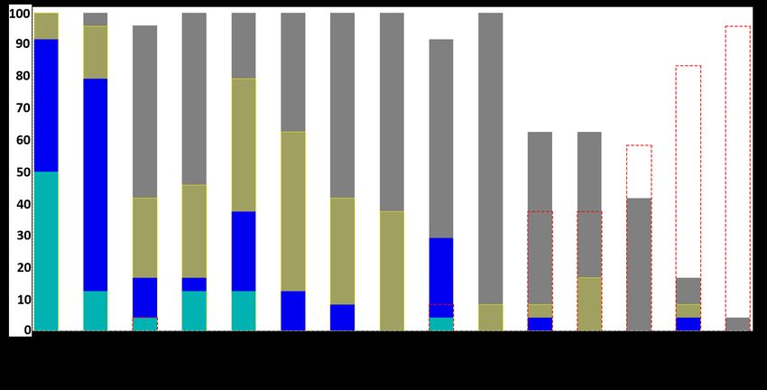
2                                                 Vicedomini, Brescia, Cavuoti et al. 2020

1 Introduction

The scientific topics covered in this work falls within what is called Time Domain
Astronomy. This is the study of variable sources, i.e. astronomical objects whose
light changes with time. Although the taxonomy of such sources is extremely rich,
there are two main kinds of objects, respectively, transients and variables. The first
changes its nature during the event, while the second presents just a brightness
variation. The study of these phenomena is fundamental to identify and analyze
either the mechanisms causing light variations and the progenitors of the various
classes of objects.
    Since ancient times the phenomenon of Supernovae (SNe) has fascinated human
beings, but only recently we understood, in most cases, why and how this explosion
happens [1]. Obviously there are still many open questions, but the knowledge about
the type of galaxy hosting various kinds of Supernova and at which rate they take
place, could help us to better understand this phenomenon and many other related
properties of the Universe [2].
    For example, the observed luminosity dispersion of SNe is evidenced through
inhomogeneities in the weak lensing event and this is an upper limit on the cosmic
matter power spectrum. Massive cosmological objects like galaxies and clusters of
galaxies can magnify many times the flux of events like SNe that would be too
faint to detect and bring them into our analysis scope. Studies on lensed SNe type
Ia by clusters of galaxies may be used to probe the distribution of dark matter on
them. Time delay between the multiple images of lensed SNe could provide a good
estimates of its high redshift. Furthermore there are two factors that makes SNe better
than other sources, like quasars, in measuring time delay [3]: (i) if the Supernovae is
taken before the peak, the measurements are easier and on short timescale compared
to the quasars; (ii) the SN light fade away with time, so we can measure the lens
stellar kinematics and the dynamics lens mass modeling. In the next decade, the Vera
C. Rubin Observatory will perform the Rubin Observatory Legacy Survey of Space
and Time (LSST), using the Rubin Observatory LSST Camera and the Simonyi
Survey Telescope. LSST will play a key role in the discovery of new lensed SNe Ia
[4]. LSST will help to find apparently host-less SNe of every type, and this may help
to study dwarf galaxies with a mass range of 104 ÷ 106 solar masses. These galaxies,
indeed, play a key role in large scale structure models, and despite their very big
predicted population, over 1 Mpc we cannot see them until now. Same story for the
theorized intracluster population of stars stripped from their galaxies, which could
be seen through the SNe host-less events.
    In order to understand and push ourselves further and further into the universe,
ever more powerful incoming observing instruments, like LSST, will be able to
deliver impressive amounts of data, for which astronomers are obliged to make an
intensive use of automatic analysis systems. Methods that fall under the heading Data
Mining and Machine Learning have now become commonplace and indispensable
to the work of scientists [5, 6, 7]. But then, where the human work is still needed?
For sure in terms of final analysis and validation of the results. This thesis work is
therefore based on this virtuous combination, by exploiting data science methodology
Machine learning based classification of transients in the era of LSST 3
and models, such as Random Forest [8], Nadam, RMSProp and Adadelta [9], to
perform a deep investigation on time domain astronomy, by focusing the attention
on Supernovae classification, performed on realistic sky simulations. Furthermore, a
special care has been devoted to the parameter space analysis, through the application
of the method ΦLAB [10, 11] to the various classification experiments, in order to
evaluate the commonalities among them in terms of features found as relevant to
solve the recognition of different types of transients.
In Sec. 2 we describe the two data simulations used for the experiments and the
extracted statistical features composing the data parameter space. In Sec. 3 we give a
brief introduction of the ML methods used, while in Sec. 4 the series of experiments
performed are deeply reported. Finally, in Sec. 5 we analyze the results and draw the
conclusions.
2 Data
In this work two simulation datasets were used; the Supernova Photometric Classifi-
cation Challenge (hereafter SNPhotCC, [12]) and the Photometric LSST Astronom-
ical Time-Series Classification Challenge (hereafter PLAsTiCC, [13, 14, 15]).
2.1 The SNPhotCC simulated catalogue
This catalogue was the subject of a challenge performed in 2010 and consists of a
mixed set of simulated SN types, respectively, Ia, Ibc and II, selected by respecting
the relative rate (Table 1). The volumetric rate was found by Dilday et al. [16] as
rv = α(1 + z)β , where for SNe Ia parameters we have αI a = 2.6 × 10⁻⁵ M pc−3 h70 3
yr , βI a = 1.5 and h70 = H0 /(70 kms M pc ). H0 is the present value of the
−1 −1 −1
Hubble parameter. For non Ia SNe, the parameters come from Bazin et al. [17]
3 yr −1 and β
and are α N onI a = 6.8 × 10⁻⁵ M pc−3 h70 N onI a = 3.6. The simulation is
based on four bands, griz, with cosmological parameters Ω M = 0.3, ΩΛ = 0.7 and
ω = −1, where Ω M is the density of barionic and dark matter, ΩΛ is the density
of dark energy and ω is the cosmological constant. Moreover, the point-spread
function, atmospheric transparency and sky-noise were measured in each filter and
epoch using the one-year chronology.
Types Bands Sampling % Amount
SNIa g,r,i,z uneven 23,86 5088
SNIbc g,r,i,z uneven 13,14 2801
SNII g,r,i,z uneven 63 13430
Table 1 SNPhotCC dataset composition.4 Vicedomini, Brescia, Cavuoti et al. 2020
SNPhotCC light curves example - g band
5
Type Ia
0
-5
-10
0
Type Ib
-5
-10
20
Type Ic
10
0
10
Type II
0
-10
56 2 40 5 62 60 56280 56300 56320 56340
MJD
Fig. 1 Examples of SNPhotCC light curves in g band. From the top to the bottom: SN004923(Ia),
SN000760(Ib), SN003475(Ic), SN001986(II).
The dataset sources are based on two variants, respectively, with or without the
host-galaxy photometric redshift. For this work only the samples without redshift
information were used.
Every simulated light curve has at least one observation, in two or more bands,
with signal-to-noise ratio > 5 and five observations after the explosion (Fig. 1). A
spectroscopically confirmed training subset was provided; it was based on observa-
tions from a 4m class telescope with a limiting r-band magnitude of 21.5 and on
observations from an 8m class telescope with a limiting i-band magnitude of 23.5.
2.2 The PLAsTiCC simulated catalogue
This catalogue arises from a challenge focused on the future use of the LSST1, by
simulating the possible objects on which science will be based. In particular, most
of these objects are transients.
LSST will be the largest telescope specialized for the Time Domain Astronomy,
whose first light is foreseen in late 2020. Its field of view will be ∼ 3.5 degrees (the
diameter will be about seven full moons side by side), with a 6.5m effective aperture,
a focal ratio of 1.23 and a camera of 3.2 Gigapixel.
1 https://www.kaggle.com/c/PLAsTiCC-2018Machine learning based classification of transients in the era of LSST 5
Every four nights it will observe the whole sky visible from the Chile (southern
emisphere). Therefore, it will find an unprecented amount of new transients: Su-
pernovae Ia, Ia-91bg, Iax, II, Ibc, SuperLuminous (SL), Tidal Disruption Events,
Kilonova, Active Galactic Nuclei, RR Lyrae, M-dwarf stellar flares, Eclipsing Bi-
nary and Pulsating variable stars, µ-lens from single lenses, µ-lens from binary
lenses, Intermediate Luminosity Optical Transients, Calcium Rich Transients and
Pair Instability Supernovae.
LSST data will be used for studying stars in our Galaxy, understanding how solar
systems and galaxies formed and the role played by massive stars in galaxy chemistry
as well as measuring the amount of matter in the Universe. PLAsTiCC includes light
curves with realistic time-sampling [15], noise properties and realistic astrophysical
sources.
Each object has observations in six bands: u (300 ÷ 400 nm), g (400 ÷ 600 nm),
r (500 ÷ 700 nm), i (650 ÷ 850 nm), z (800 ÷ 950 nm), and y (950 ÷ 1050 nm). The
training set is a mixture of what we can expect to have before LSST, so it is a quite
homogeneous ensemble of ∼ 8000 objects; the test set, instead, is based on what we
expect to have after 3 years of LSST operations and it is formed by ∼ 3, 5 million
of objects. The observations are limited in magnitude in single band to 24.5 in the r
band and to 27.8 r stacked band (see Figures 2 and 3 for examples of light curves).
By combining training and test, we collected the objects per class as listed in Table 2.
Types Training Test Bands Sampling % Amount
SNIa 2313 1659831 u,g,r,i,z,y uneven 47.57 1662144
SNIax 183 63664 u,g,r,i,z,y uneven 1.81 63847
SNIa 91bglike 208 40193 u,g,r,i,z,y uneven 1.15 40401
SNIbc 484 175094 u,g,r,i,z,y uneven 5.00 175578
SNII 1193 1000150 u,g,r,i,z,y uneven 28.65 1001343
SLSN I 175 35782 u,g,r,i,z,y uneven 1.02 35957
AGN 370 101424 u,g,r,i,z,y uneven 2.89 101794
M-Dwarf 981 93494 u,g,r,i,z,y uneven 2.68 94475
RR Lyrae 239 197155 u,g,r,i,z,y uneven 5.63 197394
Mirae 30 1453 u,g,r,i,z,y uneven 0.04 1483
Eclipse 924 96572 u,g,r,i,z,y uneven 2.77 97496
KN 100 131 u,g,r,i,z,y uneven 0.01 231
TDE 495 13555 u,g,r,i,z,y uneven 0.38 14050
µ Lens 151 1303 u,g,r,i,z,y uneven 0.04 1454
Other 0 13087 u,g,r,i,z,y uneven 0.36 13087
Table 2 PLAsTiCC dataset composition.6 Vicedomini, Brescia, Cavuoti et al. 2020
PLAsTiCC light curves example - g band
25
AGN
4
KiloNova Eclipse M-dwarf 2
500
5
Mira
50
Mu lens
500
5000
RR
TDE
5
59600 59700 59800 59900 600 00 6 01 0 0 6 0 20 0 60 300 6040 0 605 00 6060 0
MJD
Fig. 2 Examples of PLAsTiCC light curves in g band. From the top to the bottom: 2198(AGN),
2157270(M-Dwarf), 22574(Eclipsing Binary), 139362(Kilonova), 80421(Mirae), 45395(µ-lens),
184176(RR lyrae), 9197(TDE).
PLAsTiCC light curves example - g band
SN Iax SN Ia-91bg SN Ia
50
10
5
10
4
SN Ibc
2
SLSN I
200
100
SN II
50
5 98 00 5 9 90 0 60 0 0 0 60 1 0 0 602 0 0 6 030 0 6 04 00 6 05 00 60 600
MJD
Fig. 3 Examples of PLAsTiCC light curves in g band. From the top to the bottom: 15461391(SNIa),
1143209(SNIa-91bglike), 1019556(SNIax), 1076072(SNIbc), 73610(SLSN I), 1028853(SNII).Machine learning based classification of transients in the era of LSST 7
2.3 The statistical parameter space
In order to evaluate the classification performances, the light curves of the objects
have been subject of a statistical approach, by transforming them into a set of features
representing some peculiar characteristics of the astrophysical objects. Within this
work we used the following features (already used in a similar task in [18]), resulting
from a preliminary mapping of variable object light curves into a statistical parameter
space:
• Amplitude (ampl): the arithmetic average between the maximum and the mini-
mum magnitude,
magmax − magmin
ampl = (1)
2
• Beyond1std (b1std): the fraction of photometric points above or under one stan-
dard deviation from the weighted average,
b1std = P(|mag − mag| > σ) (2)
• Flux Percentage Ratio (fpr): the ratio between two flux percentiles Fn,m . The flux
percentile is defined as the difference between the flux value at percentiles n and
m, respectively. For this work, the following fpr values have been used:
f pr20 = F40,60 /F5,95
f pr35 = F32,5,67,5 /F5,95
f pr50 = F25,75 /F5,95
f pr65 = F17,5,82,5 /F5,95
f pr80 = F10,90 /F5,95
• Lomb-Scargle Periodogram (ls): the period obtained by the peak frequency of the
Lomb-Scargle periodogram.
• Linear Trend (lt): the slope a of the light curve in the linear fit,
mag = a ∗ t + b
lt = a (3)
• Median Absolute Deviation (mad): the median of the deviation of fluxes from the
median flux,
mad = mediani (|xi − median j (x j )|) (4)
• Median Buffer Range Percentage (mbrp): the fraction of data points which are
within 10% of the median flux,
mbr p = P(|xi − median j (x j )| < 0.1 ∗ median j (x j )) (5)8 Vicedomini, Brescia, Cavuoti et al. 2020
• Magnitude Ratio (mr): an index to see if the majority of data points are above or
below the median of the magnitudes,
mr = P(mag > median(mag)) (6)
• Maximum Slope (ms): the maximum difference obtained measuring magnitudes
at successive epochs,
(magi+1 − magi ) ∆mag
ms = max(| |) = (7)
(ti+1 − ti ) ∆t
• Percent Difference Flux Percentile (pdfp): the difference between the fifth and the
95th percentile flux, converted in magnitudes, divided by the median flux,
(mag95 − mag5 )
pdf p = (8)
median(mag)
• Pair Slope Trend (pst): the percentage of the last 30 couples of consecutive
measures of fluxes that show a positive slope,
pst = P(xi+1 − xi > 0, i = n − 30, ..., n) (9)
• R Cor Bor (rcb): the fraction of magnitudes that is above 1.5 magnitudes with
respect to the median,
rcb = P(mag > (median(mag) + 1.5)) (10)
• Small Kurtosis (kurt): the ratio between the 4th order momentum and the square
of the variance. For small kurtosis it is intended the kurtosis on a small number
of epochs,
µ4
kurt = 2 (11)
σ
• Skewness (skew): the ratio between the 3rd order momentum and the variance to
the third power,
µ3
skew = 3 (12)
σ
• Standard deviation (std): the standard deviation of the flux.
3 Machine Learning models
A classifier can be used as a descriptive model to distinguish among objects of
different classes, and as a predictive model to predict the class label of input patterns.
Classification techniques work better for predicting or describing data sets with
binary or nominal categories. Each technique uses a different learning algorithm
to find a model that fits the relationship between the feature set and class labelsMachine learning based classification of transients in the era of LSST 9
of the input data. The goal of the learning algorithm is to build models with good
generalization capability. The typical approach of machine learning models is to
randomly shuffle and split the given input dataset with known assigned class labels
into three subsets: training, validation and blind test sets. The validation set can be
used to validate the learning process, while the test set is used blindly to verify the
trained model performance and generalization capabilities. In the following sections
we briefly introduce the methods used to perform the classification experiments,
together with the statistical estimators adopted to evaluate their performances.
3.1 The Random Forest classifier
A Random Forest (RF, [8]) is a classifier consisting of a collection of tree-structured
classifiers {h(x, Θk ), k = 1, ...} where the {Θk } are independent identically dis-
tributed random vectors and each tree casts a unit vote for the most popular class
at input x [19]. The generalization error for this algorithm depends on the strength
of single trees and from their correlations through the raw margin functions. The
upper bound, instead, tell us that smaller the ratio of those quantities, better the RF
performance. To improve the model accuracy by keeping trees strength, the corre-
lation between trees is decreased and bagging with a random selection of features
is adopted. Bagging or Bootstrap Aggregating, is a method designed to improve the
stability and accuracy of machine learning algorithms. It also reduce variance and
minimizes the risk of overfitting. Given a training set of size n, bagging generates
m new training sets, each of size p, by sampling from the original one uniformly
and with replacement. This kind of sampling is known as a bootstrap sample. The
m models are fitted using the m bootstrap samples and combined by averaging the
output (for regression) or voting (for classification). Bagging is useful because, in
addition to improving accuracy when using random features, it provides an estimate
of the generalized error of the set of trees and the strength and correlation of trees.
The estimation is done out-of-bag. Out-of-bag means that the error estimate of each
pair (x,y) is made on all those bagging datasets that do not contain that given pair.
3.2 The Nadam, RMSProp and Adadelta classifiers
The simplest optimization algorithm is the Gradient Descent, in which the gradient
of the function to be minimized is calculated. This depends on the parameter θ t−1 .
Only a portion of the gradient is used to update the parameters; this portion is given
by the parameter η:
g ←− ∇θt −1 f (θ t−1 − ηµmt−1 )
t
mt ←− µmt−1 + gt
θ t ←− θ t−1 − ηmt
10                                                   Vicedomini, Brescia, Cavuoti et al. 2020

    where m is the so-called momentum vector, used to accelerate the update of the
learning function, while µ is the decay constant. These two terms increase the speed
of gradient decreasing in the direction where the gradient tends to remain constant,
while reducing it where the gradient tends to oscillate.
    Nadam is a modified version of the Adam algorithm, based on the combination
between the momentum implementation and the L2 normalization. This type of
normalization changes the η member, dividing it by the L2 norm of all previous
gradients.
    Adadelta is a variant that tries to reduce the aggressive, monotonically decreasing
learning rate. In fact, instead of accumulating all past squared gradients, it restricts the
window of accumulated past gradients to some fixed size w. This has the advantage
of compensating for the speeds along the different dimensions by stabilizing the
model on common features and allowing the rare ones to emerge. A problem of
this algorithm comes from the norm vector that could become so large to stop the
training, preventing the model from reaching the local minimum. This problem is
solved by RMSProp, a L2 normalization based algorithm, which replaces the sum of
nt with a decaying mean, characterized by a costant value ν. This allows the model
to avoid any stop of the learning process. For a detailed description of these models,
see [9].

3.3 Parameter Space exploration

The choice of an optimal set of features is connected to the concept of feature impor-
tance, based on the measure of a feature’s relevance [11]. Formally, the importance
or relevance of a feature is its percentage of informative contribution to a learning
system. We approached the feature selection task in terms of the all-relevant feature
selection, able to extract the most complete parameter space, i.e. all features consid-
ered relevant for the solution to the problem. This is appropriate for problems with
highly correlated features, as these features will contain nearly the same informa-
tion. With a minimal-optimal feature selection, choosing any one of them (which
could happen at random if they are perfectly correlated), means that the rest will
never be selected. The method ΦLAB, deeply discussed in [11], includes properties
of both embedded and wrappers categories of feature selection to optimize the pa-
rameter space, by solving the all-relevant feature selection problem, thus indirectly
improving the physical knowledge about the problem domain.

3.4 Classification statistics

In this work, the performance of the classification models is based on some statistical
estimators, extracted from a matrix known as confusion matrix [20].
Machine learning based classification of transients in the era of LSST 11
Predicted
P=0 N=1
p=0 a00 a10
Target
n=1 a01 a11
Table 3 Example of a binary confusion matrix.
The example shown in Table 3 is a confusion matrix for a binary classification.
Each entry ai j in this table is the number of records from class i predicted to
be of class j. The numbers a00 and a11 show correct classified records. The a01
records named False Positive indicate wrong records classified in class 0, when their
correct classification was class 1; instead, a10 named False Negative show the records
classified in class 1 but belonging to class 0. The total number of correct predictions
is a11 + a00 , and the total number of wrong ones is a10 + a01 . For a better comparison
between different models, summarizing the results through a confusion matrix is the
common way. We can do this using a performance metric, such as accuracy, defined
as follows:
a00 + a11
Accuracy =
a00 + a11 + a01 + a10
A highest accuracy is the target of every classifier. Other important statistical
estimators, for a better understanding of the results for each class, are:
TruePositive
Purit y =
TruePositive + FalsePositive
TruePositive
Completeness =
TruePositive + FalseNegative
FalsePositive
Contamination = 1 − Purit y =
TruePositive + FalsePositive
2
F1Scor e =
(Purit y)−1 + (Completeness)−1
Purity of a class is the percentage of correctly classified objects in that class,
divided by the total classified objects in that class. Also named as precision of a
class.
Completeness of a class is the percentage of the correctly classified objects in that
class divided by the total amount of objects belonging to that class. Also named as
recall of a class.
Contamination of a class is the dual measure of purity.
F1-Score of a class is the harmonic mean between purity and completeness of that
class and it is a measure of the average trade-off between purity and completeness.12 Vicedomini, Brescia, Cavuoti et al. 2020
4 Experiments
In order to pursue the main goal of the present work, related to a deep analysis of SNe
in terms of their classification and characterization of the parameter space required
to recognize their different types, we relied on the two simulation datasets, one in
particular developed and specialized within the LSST project (see Sections 2.1 and
2.2). We preferred a statistical approach, by mapping the light curves into a set of sta-
tistical features. The classification with statistical data have been performed through
the comparison of different types of classifiers, respectively, Nadam, RMSProp,
Adadelta and Random Forest.
A data pre-processing phase was carried out on the PLAsTiCC dataset, based on
a pruning on the flux and related error, in order to reduce the amount of negative
fluxes present within data, which could affect the learning capability of the machine
learning models. On the SNPhotCC dataset, both the errors in the flux and the
quantity of negative fluxes were such that it was not deemed necessary to perform
the pruning. The curves in the PLAsTiCC dataset were selected in successive steps
so as to minimize the presence of negative fluxes, reaching, where possible, a subset
of about 35,000 light curves per type. In the SNPhotCC dataset, on the other hand,
all the given 5088 SN-Ia curves were selected and the type II curves were reduced
so as to balance the classes; the other types of SNe have been discarded, due to their
negligible amount available.
The sequence of classification experiments followed an incremental complexity,
starting from the most simple exercise on the PLAsTiCC dataset, i.e. the separation
between periodic and non-periodic objects (P Vs NP), expected to be well classified
due to their very different features within any parameter space. In terms of initial
minimization of negative fluxes, it was decided to apply the following replacement:
for each class of objects, the observations related to the same day were grouped, by
taking the least positive flux value. This value has been replaced to all the negative
fluxes of that day.
As expected, the classifiers revealed a high capability to disentangle periodic
from non-periodic objects. Therefore, in all further experiments we excluded peri-
odic sources, by focusing the exclusive attention to variable objects, increasing the
complexity of classification, by considering different sub-classes of transients and
evaluating the performances of the selected machine learning classifiers.
The next step was, in fact, to recognize the SNe from all the other non-periodic
objects available in the dataset (SNe Vs All). But, preliminarly, we tested different
methods for replacing the negative fluxes. For instance, in addition to the first men-
tioned method (e.g. minimum positive flux extracted from observations within the
same day), a second method was chosen, in which negative fluxes were replaced
by the constant number 0.001, considered as the absolute minimum flux emitted by
the sources. We tried also a third method, in which the negative fluxes were sim-
ply excluded from the input dataset, without any replacement. In theory, such third
method was considered the worst case, since it would cause a drastic reduction of
the light curve sample available. As we will show, the second method (the constantMachine learning based classification of transients in the era of LSST 13 minimum flux value), obtained the best classification performances for all classifiers. Therefore, it was used as the reference for all further classification experiments. The subsequent experiments concerned some fine classifications of most interest- ing SNe types, starting from the classic case of SNIa Vs SNII types, followed by a mix of SNIa Vs Superluminous SNe I (SNIa Vs SL-I), concluding with the most com- plex case, based on the multi-class experiment, in which we tried to simultaneously classify all six different types of SNe (six-class SNe). Fig. 4 Summary of the procedure designed and followed along the experiments. Besides the negative flux replacement, we investigated also the feature selection problem, in order to identify the most significant parameter space able to recognize different types of SNe. After the selection process we verified that such reduced
14                                                 Vicedomini, Brescia, Cavuoti et al. 2020

amount of data dimensions could maintain sufficiently high the classification per-
formances. We tried also to maintain uniform the number of features among the
different use cases, although respecting their statistical importance, exploring the
possibility to find a common parameter space, suitable for all classification cases.
   The SNIa Vs SNII use case was also performed on the SNPhotCC dataset, since
this dataset was composed almost exclusively by such two types of SNe. The results
were then compared with those performed on the PLAsTiCC dataset, deprived of the
u and y bands for uniformity with the SNPhotCC dataset bands, in order to maximize
the fair comparison.
   In summary, in this work five series of experiments were performed on the
PLAsTiCC dataset and one on the SNPhotCC dataset. Such experiments were chosen
hierarchically and considering the most important goal of this work, i.e. the fine
classification of SNe types. An overview of the followed procedure is shown in
Fig. 4.

4.1 Data pre-processing

From the whole PLAsTiCC dataset a maximum of 200, 000 objects per class was
randomly extracted (whenever possible). For each class, a pruning in flux and its
error was performed. While, no any pruning was done on the SNPhotCC dataset.
The Table 4 shows the limits derived from pruning.
    After this first skimming, the amount of objects for the various classes was reduced
to a maximum of about 35, 000 curves. The reduction for classes with more than 35K
objects was driven by the choice of the curves with the least number of observations
with negative fluxes and with at least 6 observations per band.
    Due to the residual presence of negative fluxes, we started their handling by
trying the following replacement method. By considering all the curves of a class,
we checked all the observations of a given day. If in that day there was a negative
or zero flux, then it was replaced with the lowest positive flux present. Else if only
negative fluxes were present, they were replaced with the lowest positive flux of the
previous day. This replacement has been applied to every day, for all curves and for
all classes. An example of the replacing method is shown in Table 5.
    Since 19 features have been chosen for our statistical approach, by considering 6
bands in PLAsTiCC, a total of 114 features composed the original parameter space.
    After the composition of statistical datasets, some light curves included some
missing entries, or NaN (Not-a-Number), causing the exclusion of those objects
from the datasets, due to their unpredictable impact on the training of classifiers.
The total amount of light curves per class is reported in Table 6.
Machine learning based classification of transients in the era of LSST 15
Object Band Flux Flux Error Object Band Flux Flux Error
u > -50 -60 -50 -60 -50 -60 -50 -60 -200 -10 -800 -10 -900 -10 -800 -10 -1100 -20 -800 -30 -30 -40 -20 -20 -50 -30 -1200 -40 -8000 -60 -11000 -90 -1300 -50 -6000 -20 -6000 -20 -4500 -40 -4500 -60 -5500 -100 -30 -30 -10 -20 -20 -20 -30 -30 -50 -40 -90 -90 -50 -40 -20 -20 -20 -20 -30 -30 -60 -60 -110 -110 -30 -20 -10 -10 -15 -10 -20 -20 -40 -30 -70 -6016 Vicedomini, Brescia, Cavuoti et al. 2020
ID MJD Flux
Before After
1 59820.0015 −25.154862 0.284215
2 59820.0238 15.458932 15.458932
3 59820.1234 −5.848961 0.284215
4 59820.4451 −20.548951 0.284215
5 59820.8251 0.284215 0.284215
6 59820.0234 −9.542318 0.284215
7 59820.6234 10.854215 10.854215
Table 5 Example of the negative fluxes replacement within the PLAsTiCC catalogue.
Dataset Object Curves Object Curves
AGN 34666 E. Binary 34484
Kilonova 232 M-Dwarf 34849
Mirae 1154 µ Lens 1187
PLAsTiCC RR Lyrae 32698 SN Ia 34953
SN Iax 34977 SN Ia 91bg 34923
SN Ibc 34932 SN II 34828
SL SN I 34959 TDE 14023
Total objects 361711
SNPhotCC SNIa 5088 SNII 12027
Total objects 17115
Table 6 Summary of the light curves composing the simulated datasets.
class, as shown in Table 7. The random partitioning percentage between training and
test sets was fixed, respectively, to 80% and 20%.
Number of curves Number of curves
Object Object
Training Test Training Test
RR Lyrae 26158 6540 Kilonova 187 46
E. Binary 27587 6897 M-Dwarf 6001 1501
Mirae 923 231 µ Lens 950 238
AGN 6001 1501 SN Ia 6001 1501
SN Iax 6001 1501 SN Ia 91bg 6001 1501
SN Ibc 6001 1501 SN II 6001 1501
SL SN I 6001 1501 TDE 6001 1501
Total P Training 54668 Total NP Training 55146
Total P Test 13668 Total NP Test 13793
Table 7 Summary of the sources belonging to the PLAsTiCC dataset in the P (periodic class) Vs
N P (non periodic class) use case divided in training (80%) and test (20%) sets.
This series of experiments, as expected, being the simplest given the intrinsic
difference of the objects involved, did not reveal any surprise. All estimators showed
a great efficiency to recognize periodic objects from the variables (non periodic)
ones.Machine learning based classification of transients in the era of LSST 17
% type RF Nadam RMSProp Adadelta
Accuracy - 99 97 98 96
NP 99 97 99 95
Purity
P 99 98 98 97
NP 99 98 98 97
Completeness
P 99 97 99 95
NP 99 98 98 96
F1 Score
P 99 97 98 96
Table 8 Summary of the best results (in percentages) for the 4 classifiers in the classification
experiment P Vs NP. For Nadam, RMSProp and Adadelta models, a decay value of 10−5 and a
learning rate of 0.0005 were assigned.
4.3 Handling of negative fluxes
In both simulated catalogues, as introduced in Sec. 4, the presence of negative fluxes
required an investigation on how to replace them in order to minimize their negative
impact on the learning efficiency of machine learning models. Therefore, it was
decided to approach this problem in three ways.
The first (named as M1) was to replace their value as introduced in Sec. 4
(and preliminarly used for the Periodic Vs Non Periodic classification experiment,
described in Sec. 4.2): for each class of objects, the observations related to the
same day were grouped, by taking the least positive flux value. This value has been
replaced to all the negative fluxes of that day.
The second approach (named as M2) was to replace the negative fluxes with a
constant value of 0.001, considered as the minimum flux emitted by the sources.
The third solution (M3) consisted into the total rejection of negative fluxes from
the dataset, without any replacement.
The impact on classification accuracy has been analyzed by comparing the three
solutions in the SNe Vs All (the class All includes the rest of transient types) classi-
fication experiment on the Plasticc dataset and the SNIa Vs SNII experiment on the
SNPhotCC dataset. In both cases, the data have been treated with the three replace-
ment types, producing different amount of objects per class. The entire composition
of the datasets for the three methods is shown in Table 9, while the composition of
the classes of SN, All, SNIa and SNII are shown in Table 10.
The results of the two experiments are shown, respectively, in Tables 11 and 12.
The results indicated that, on average, in the case of the PLAsTiCC dataset, the
second method (M2) obtained a better accuracy, with some exception in favor of
M3. In the case of SNPhotCC dataset, on the other hand, M2 and M3 resulted more
close in terms of classification efficiency. Therefore, since we were mostly interested
to directly compare the classification performances between the two datasets, by
considering also the drastic reduction of available sources using the M3 method, we
definitely selected and applied the M2 to both datasets.18 Vicedomini, Brescia, Cavuoti et al. 2020
Object Number of curves Object Number of curves
M1 M2 M3 M1 M2 M3
AGN 34666 34666 34082 Kilonova 232 232 229
µ Lens 1187 1187 1144 M-Dwarf 34849 34849 34191
SN Ia 34953 34891 34423 SL SN I 34959 34959 34750
PLAsTiCC
SN Iax 34977 34977 34680 SN Ia 91bg 34923 34923 34559
SN Ibc 34932 34932 34437 SN II 34828 34771 34393
TDE 14023 14023 13985
Total objects M1: 294529 Total objects M2: 294410 Total objects M3: 290873
SNPhotCC SNIa 5088 5088 5086 SNII 5088 5088 5077
Total objects M1: 10176 Total objects M2: 10176 Total objects M3: 10163
Table 9 Summary of sources of datasets for each replacing method adopted for negative fluxes.
M1 M2 M3
Object Training Test Training Test Training Test
AGN 27732 6934 27732 6934 27266 6816
Kilonova 186 46 186 46 183 46
µ Lens 949 238 949 238 915 229
M-Dwarf 27879 6970 27879 6970 27353 6838
SN Ia 12001 3001 11975 2994 11802 2954
PLAsTiCC SL SN I 12001 3001 12001 3001 11935 2979
SN Iax 12001 3001 12001 3001 11900 2976
SN Ia 91bg 12001 3001 12001 3001 11866 2975
SN Ibc 12001 3001 12001 3001 11828 2951
SN II 12001 3001 11983 2992 11835 2970
TDE 11218 2805 11218 2805 11188 2797
Total SN 72006 18006 71962 17990 71166 17805
Total All 67964 16993 67964 16993 66905 16726
SNIa 4071 1017 4071 1017 4062 1016
SNPhotCC
SNII 4071 1017 4071 1017 4070 1015
Table 10 Summary of sources of training and test sets for each negative flux replacing method.
4.4 Optimization of the Parameter Space for transients
After choosing how to handle the negative fluxes, we investigated the statistical
parameter space (PS) of the two simulated datasets, in order to explore the possibility
to reduce the dimensionality of the classification problem (feature selection) and to
analyze the impact of the resulting optimized PS on the classification efficiency for
each particular type of classes involved in all cases, as well as the possibility to find
a common set of relevant features, suitable to separate different types of transients.
We applied the ΦLAB algorithm, introduced in Sec. 3.3, to both datasets in various
classification use cases (except the preliminary experiment P Vs NP), obtaining an
optimized parameter space for each of them. The analysis of feature commonalities
among all classification experiments is shown in Fig. 5. In particular, the feature
selection of the SNIa Vs SNII use case has been done on the PLAsTiCC datasetMachine learning based classification of transients in the era of LSST 19
Dataset Use case Algorithm Class Estimator M1 M2 M3
Purity 86 91 85
SN Completeness 94 93 91
F1-score 90 92 88
RF
Purity 93 92 90
All Completeness 83 90 83
F1-score 88 91 86
Purity 77 84 83
SN Completeness 82 78 85
F1-score 79 81 84
Nadam
Purity 80 78 84
All Completeness 73 85 82
F1-score 76 81 83
PLAsTiCC SNe Vs All
Purity 85 89 87
SN Completeness 83 89 91
F1-score 84 89 89
RMSProp
Purity 83 88 90
All Completeness 85 89 86
F1-score 84 88 88
Purity 80 85 85
SN Completeness 84 86 87
F1-score 82 86 86
Adadelta
Purity 82 85 86
All Completeness 78 84 84
F1-score 80 85 85
Table 11 Comparison among the three replacing methods for negative fluxes on the PLAsTiCC
dataset in the classification case SNe Vs All. For Nadam, RMSProp and Adadelta a learning rate of
0.001 and a decay value of 10−5 were chosen. The statistics are expressed in percentages.
deprived of the u and y bands, for uniformity with the SNPhotCC dataset in terms
of direct comparison.
From the analysis of the histogram of Fig. 5 it was possible to extract a common
optimized parameter space, composed by relevant features with higher percentage
of common occurrences among various classification use cases (the cumulative
measurement process is explained in the caption of the Fig. 5). The extraction was
done trying also to balance the different amount of relevant features provided by
ΦLAB in every classification case with their percentage of commonality among
different cases, with the aim at extracting the same number of relevant features in
all cases. The best compromise found is reported in Table 13 and corresponds to
78 extracted features (on a total of 114) suitable for the six-band cases (ugrizy in
PLAsTiCC) and 52 (on a total of 76) for the four-band cases (griz in SNPhotCC).
These two resulting optimized (reduced) parameter spaces have been used in the
classification cases described in the next sections, each time by comparing the
classification efficiency between the complete and the reduced parameter spaces.
By looking at the optimized parameter spaces obtained (Fig. 5), extremely inter-
esting is the presence of some common features among the various classification
cases. In particular, the Amplitude (ampl) shows a crucial role for the classification
of various SNe types. Also important is the Standard Deviation (std), which reaches20 Vicedomini, Brescia, Cavuoti et al. 2020
Dataset Use case Algorithm Class Estimator M1 M2 M3
Purity 91 95 91
SNIa Completeness 94 97 93
F1-score 93 96 92
RF
Purity 94 97 93
SNII Completeness 91 95 91
F1-score 92 96 92
Purity 86 91 92
SNIa Completeness 92 92 94
F1-score 89 92 93
Nadam
Purity 91 92 94
SNII Completeness 86 91 92
F1-score 88 91 93
SNPhotCC SNIa Vs SNII
Purity 91 92 93
SNIa Completeness 93 96 94
F1-score 92 94 94
RMSProp
Purity 93 96 94
SNII Completeness 91 92 93
F1-score 92 94 94
Purity 89 86 92
SNIa Completeness 92 88 92
F1-score 91 87 92
Adadelta
Purity 92 88 92
SNII Completeness 89 85 92
F1-score 90 87 92
Table 12 Comparison among the three replacing methods for negative fluxes on the SNPhotCC
dataset in the classification case SNIa Vs SNII. For Nadam, RMSProp and Adadelta a learning rate
of 0.001 and a decay value of 10−5 were chosen. The statistics are expressed in percentages.
Feature [SNe Vs All] [SNIa Vs SNII] [SNIa Vs SL-I] [six-class SNe] | [SNIa Vs SNII]
PLAsTiCC | SNPhotCC
ampl b a nd x x x x x
pdfp b a nd x x x x
ms b a nd x
mad b a nd x x x x x
std b a nd x x x x x
skew b a nd x x x x x
fprXX b a nd x x x x x
kurt b a nd x x x x x
ls b a nd x x x x x
lt b a nd x x x x x
Totals PLAsTiCC: 78 SNPhotCC: 52
Table 13 Summary of the resulting common optimized parameter spaces from the analysis of
the feature selections. Each feature listed is intended to include all its available bands. First four
use cases (columns 2 to 5) refer to the classification cases approached on PLAsTiCC with such
optimized PS in six bands (ugrizy), while last column is referred to the classification experiment
done with SNPhotCC in four bands (griz). For PLAsTiCC the optimized PS include 78 features,
while SNPhotCC is composed by 52. Take into account that the feature fprXX b a nd includes 5
different types per band group (See Sec. 2.3 for details).Machine learning based classification of transients in the era of LSST 21
Fig. 5 Cumulative statistical analysis of the feature selection performed with the method ΦLAB
on different use cases. The results include the four classification cases on PLAsTiCC (SN Vs All,
SNIa Vs SNII, SNIa Vs SL-I, six-class SNe) and the single case SNIa Vs SNII on SNPhotCC.
The indicated features are grouped per statistical type, including all their available bands. After
having calculated the various feature rankings for each classification case with ΦLAB, ordered by
decreasing importance, the vertical bars shown in the histogram represent the percentage of common
occurrences of each feature type, among various classification use cases, within, respectively, the
first 25% (cyan), 50% (blue), 75% (yellow) and 100% (gray) of feature rankings. While dotted red
bars indicate the percentage of common occurrences of rejection among various feature rankings.
79.2% of common occurrences. Equally interesting appears the high percentage of
common rejections of Median Buffer Range Percentage (mbrp), Magnitude Ratio
(mr) and R Cor Bor (rcb). Within most of the light curves of the datasets used, the
average value of the mbrp, which is the percentage of points in an interval of 10% of
the median flux, is very high. This shows that most of the light curves are relatively
contained within the flux extension. The mr feature, the percentage of points above
the median magnitude, has always values greater than 40%, with a standard devia-
tion of a lower order of magnitude, except in the case of the six-class SNe problem,
in which the standard deviation is comparable with the mr value. This shows that
most of the light curves are basically symmetrical in magnitude. Finally, the rcb has
an average value of about 30% with a comparable standard deviation. Therefore, it
ranges over the whole spectrum of possible values without any class distinction.
The ampl, which from a physical point of view represents the half-amplitude, in
magnitude, of the light curves, is the most important feature in all use cases and it
is related to the different distribution of objects in the classes. In the SNe Vs All use
case, the class of SNe shows a bi-modal distribution, while the class All shows an
alternation between bi-modal and uni-modal distributions, with different peaks from
the SNe distributions. In the SNIa Vs SL-I use case, the SNe Ia have a bi-modal
distribution, unlike the SL-I type, which instead is uni-modal. The six-class SNe use
case shows that the SNe Ia have a similar peak w.r.t. the sub-types Iax, Iabg91, SL
and the Ibc. The SNe II instead, show an unexpected shape similarity with the SNe22 Vicedomini, Brescia, Cavuoti et al. 2020
Ia in the PLAsTiCC simulation, and this should explain a classification efficiency
in the SNIa Vs SNII case smaller than what obtained on the SNPhotCC data (see
Sec. 4.6).
The std, the deviation from the mean flux, has the same trend of the ampl, with
bi-modal and uni-modal distributions and with peaks at different values.
The fpr, the flux percentage ratio, related to the sampling of the light curve
assuming a relevance with the higher flux values, shows that, in the SNe Vs All case
and with the griz bands, there are two distributions with distinguishable peaks. In the
six-class SNe case, the riz bands, with the wider flux ratios, contribute to solve the
envelope of the 6 classes. In the SNIa Vs SL-I case, the different distributions can be
particularly identified in the rizy bands, again in the broader flux ratios such as 50,
65 and 80. Finally, in the SNIa Vs SNII problem the distinction is more complex and
only in few riz band cases it is possible to see the two different distributions.
In the other relevant features shown in Fig. 5, we do not infer distinct distributions
in the various use cases, but only different fluctuations around the same distribution.
This means that all the curves of all the classes share, more or less, the same
distribution w.r.t. the flatness of the curve (kurt), the symmetry of the curve (skew),
the slope deriving from the linear fit (lt), the period obtained from the peak frequency
of the Lomb Scargle Periodogram (ls), the ratio of difference between percentiles and
the median (pdfp) and finally the median of deviations from the median (mad). Since
these features have proved to be highly relevant, this implies that those fluctuations
in the class distributions contribute substantially to the classification of different
types of SNe. Finally, in the six-class SNe problem, another feature appears relevant,
which is the maximum difference in magnitude between two successive epochs (ms),
providing, slightly in the u band and in a more consistent way in the y one, fluctuations
suitable in principle for the resolution of the more complex classification.
4.5 Supernovae versus All
In this use case we had SNe type Ia, Iax, Ia 91bg-like, Ibc, II and SL-I within the
SNe class and all the other object types, except the excluded periodic ones, in the All
class. We performed the experiments on the PLAsTiCC dataset with the 4 classifiers
using, respectively, the entire set of statistical features available (114) and with the
optimized parameter space (78). The amount of objects for each type included in the
two classes is shown in Table 14.
Among Nadam, RMSProp and Adadelta, the best performances were obtained
with the RMSProp in both cases (whole and optimized parameter spaces). While
Random Forest reached the best classification performances. The statistical results
are shown in Table 15.Machine learning based classification of transients in the era of LSST 23
Type Training Test
SN Ia 11975 2994
SN Iax 12001 3001
SN Ia91bg 12001 3001
SN Ibc 12001 3001
SN II 11983 2992
SL SN I 12001 3001
Kilonova 186 46
M-Dwarf 27879 6970
µ Lens 949 238
TDE 11218 2805
AGN 27732 6934
Total SN 71962 17990
Total All 67964 16993
Table 14 Summary of the objects belonging to the PLAsTiCC dataset, used for the SNe Vs All
experiment, randomly partitioned in training (80%) and test (20%) sets.
Random Forest Nadam RMSProp Adadelta
Features All 78 All 78 All 78 All 78
% Accuracy - 92 92 85 86 90 90 86 85
SN 91 91 85 86 91 91 86 84
% Purity
All 92 92 85 86 89 90 86 86
SN 93 93 86 87 90 90 87 87
% Completeness
All 90 90 84 85 90 90 85 83
SN 92 92 86 87 90 87 87 86
% F1 Score
All 91 91 84 86 90 86 86 84
Table 15 Summary of the statistical results for the 4 classifiers with, respectively, all the features
and the 78 selected. For Nadam, RMSProp and Adadelta, the values of 10−5 and 0.0005 were
assigned to the decay and learning rate hyper-parameters, respectively.
4.6 Supernovae Ia versus II
In this experiment we considered only SNe of type Ia and II. In this case it was possi-
ble to use both SNPhotCC and PLAsTiCC datasets, since in the case of SNPhotCC,
these two types of SN were available. The amount of objects used is shown in
Table 16.
Number of curves
Dataset Type
Training Test
SN Ia 27964 6990
PLAsTiCC
SN II 27983 6966
Total 55947 13956
SN Ia 4071 1017
SNPhotCC
SN II 4071 1017
Total 8142 2034
Table 16 Summary of the objects belonging to the datasets used for the SNIa Vs SNII experiment
on PLAsTiCC and SNPhotCC, randomly partitioned in training (80%) and test (20%) sets.24 Vicedomini, Brescia, Cavuoti et al. 2020
We performed the experiment with the 4 classifiers using, respectively, all the
features and the amounts related to the two optimized feature sets, respectively, 78 for
PLAsTiCC and 52 for SNPhotCC. For a direct comparison between the SNPhotCC
and PLAsTiCC datasets, we also considered a reduced version of the PLAsTiCC
dataset, by excluding the u and y bands for uniformity with the SNPhotCC catalogue
in terms of bands available. The statistical results are reported in Table 17.
Random Forest Nadam RMSProp Adadelta
PLA SNP PLA SNP PLA SNP PLA SNP
Bands used 6 6 4 4 4 6 6 4 4 4 6 6 4 4 4 6 6 4 4 4
Features All 78 52 All 52 All 78 52 All 52 All 78 52 All 52 All 78 52 All 52
% Accuracy - 78 79 78 96 96 71 72 71 93 94 76 76 78 94 96 74 74 73 90 95
Ia 76 76 76 95 95 70 70 69 90 92 74 74 75 93 94 72 73 72 89 93
% Purity
II 81 81 80 97 97 72 73 74 95 96 78 78 80 95 98 75 74 75 92 96
Ia 82 83 82 97 97 75 76 77 96 96 79 80 82 95 98 76 75 77 92 96
% Completeness
II 74 74 74 95 95 67 67 65 89 92 73 71 73 93 93 71 72 70 88 93
Ia 79 79 79 96 96 72 73 73 93 94 77 77 79 94 96 74 74 74 90 95
% F1 Score
II 77 78 77 96 96 70 70 69 92 94 75 74 76 94 95 73 73 72 90 95
Table 17 Summary of the statistical results for the 4 classifiers in the SNIa Vs SNII experiment. For
each classifier it is reported the statistics related to the PLAsTiCC (PLA columns) and SNPhotCC
(SNP columns) datasets. In the case of PLAsTiCC, the columns are related to the whole original
feature space (All) and the optimized one (78) using 6 bands (ugrizy), together with the reduced
feature space (52) using 4 bands (griz) for a direct comparison with the corresponding optimized
parameter space obtained on SNPhotCC. For Nadam, RMSProp and Adadelta, the values of 10−5
and 0.0005 were assigned to, respectively, the decay and learning rate hyper-parameters, in the
cases of 78 features. While 10−5 and 0.001 values have been assigned for the cases with 52 features.
In terms of classification performance, it appears evident the discrepancy between
the two datasets. The capability of classifiers to recognize the two classes is higher on
SNPhotCC and this implies a strong dependency of learning models from the overall
accuracy of the simulations. Furthermore, the very similar percentages among the
whole feature set and the optimized versions probes the capability of the feature
selection method ΦLAB to extract a set of relevant features, able to preserve the
level of classification efficiency.
4.7 Superluminous SNe versus SNe I
In the SNIa Vs SL-I experiment, the three sub-classes of SNe, Ia, Ia91bg and Iax
have been mixed in the same percentage and then classified against Superluminous
SNe I. We performed the experiments with the 4 classifiers using all the features and
the 78 selected with ΦLAB. The amount of objects per type is shown in Table 18.
The statistical results of the classification are shown in Table 19.
By analyzing the results, it is noticeable the lower performance of Adadelta w.r.t.
other classifiers, where Random Forest appeared the best one for all estimators. TheMachine learning based classification of transients in the era of LSST 25
Number of curves
Type
Training Test
SN Ia 9323 2331
SN Iax 9323 2331
SN Ia91bg 9323 2331
SLSN I 27967 6992
Total Ia 27969 6993
Total SL 27967 6992
Table 18 Summary of the objects belonging to the dataset used for the SNIa Vs SL-I experiment
on PLAsTiCC, randomly partitioned in training (80%) and test (20%) sets.
Random Forest Nadam RMSProp Adadelta
Features All 78 All 78 All 78 All 78
% Accuracy - 88 87 81 82 85 82 71 70
SL-I 83 80 77 74 81 77 71 70
% Purity
SN Ia 93 93 85 89 90 87 71 70
SL-I 94 95 87 92 91 89 71 70
% Completeness
SN Ia 80 76 74 69 79 74 72 71
SL-I 88 87 82 82 86 83 71 70
% F1 Score
SN Ia 86 84 79 78 84 80 71 70
Table 19 Summary of the statistical results for the 4 classifiers on the SNIa Vs SL-I experiment,
with, respectively, all the features and the 78 of the optimized parameter space of PLAsTiCC
dataset. For Nadam, RMSProp and Adadelta, the values of 10−5 and 0.0005 were assigned to the
decay and learning rate hyper-parameters, respectively.
similar results obtained for both parameter spaces confirm the validity of the feature
selection.
In terms of error percentages on the SN I class (all Ia sub-types), Table 20 reports
the level of contamination for each sub-type in the experiment with all features and
using Random Forest.
Correctly
Class Total Wrongly classified
classified
SN Ia 2331 2328 3 ≈ 0%
SN Iax 2331 1508 823 35%
SN Ia91bg 2331 1779 552 24%
Table 20 Summary of the contamination analysis among all SN Ia sub-types obtained by the
Random Forest, with the complete parameter space, on the SNIa Vs SL-I experiment.
As shown in Table 20, the most contaminated sub-class is SNIax, which indicates
its high difficulty of recognition among other SN types.26 Vicedomini, Brescia, Cavuoti et al. 2020
4.8 Simultaneous classification of six SNe sub-types
Last classification experiment performed was the most complex, because we tried to
classify simultaneously all the six classes of SNe available in the PLAsTiCC dataset.
The experiments with the 4 models were performed using all the features and the 78
selected by the optimization procedure. The amount of objects per class is shown in
Table 21.
Number of curves
SN Class
Training Test
Ia 27912 6979
Ia91bg 27938 6985
Iax 27981 6996
II 27816 6955
Ibc 27945 6987
SL I 27967 6992
Table 21 Summary of the objects belonging to the dataset used for the six-class SNe experiment
on PLAsTiCC, randomly partitioned in training (80%) and test (20%) sets.
The statistical results of the six-class classification is reported in Table 22.
Random Forest Nadam RMSProp Adadelta
Features All 78 All 78 All 78 All 78
% Accuracy - 66 62 53 55 60 61 48 48
SN Ia 79 79 68 71 73 76 62 59
SN Ia 91bg 82 78 64 70 79 81 52 58
SN Iax 58 57 46 48 52 51 39 34
% Purity
SN II 74 75 58 61 68 66 56 55
SN Ibc 40 42 32 34 34 35 32 32
SL SN I 62 59 48 47 56 56 47 50
SN Ia 77 77 56 57 68 67 55 48
SN Ia 91bg 25 30 27 20 20 17 21 16
SN Iax 33 37 16 20 26 27 21 15
% Completeness
SN II 79 79 79 77 77 78 67 67
SN Ibc 64 57 47 47 54 58 38 47
SL SN I 91 91 76 88 88 85 85 87
SN Ia 78 78 62 63 71 71 58 53
SN Ia 91bg 39 44 38 31 32 28 30 26
SN Iax 42 45 23 29 35 35 27 21
% F1 Score
SN II 76 77 67 68 72 72 61 60
SN Ibc 49 48 38 40 42 44 34 38
SL SN I 73 72 59 62 68 67 61 63
Table 22 Summary of the statistical results for the 4 classifiers on the six-class SNe experiment,
with, respectively, all the features and the 78 of the optimized parameter space of PLAsTiCC
dataset. For Nadam, RMSProp and Adadelta, the values of 10−4 and 0.001 were assigned to the
decay and learning rate hyper-parameters, respectively.Machine learning based classification of transients in the era of LSST 27
Also in this case, the Random Forest obtained best results and the similar statistics
between the whole and optimized parameter space confirm the good performances
of the feature selection method. By analyzing the classification estimators for the
single classes, the SNIa91bg showed a high difficulty to be recognized, while Ia91bg
and Iax types were often confused for SNIbc. SL type resulted the most complete,
although the purity was reduced by the contamination of SNIbc and SNIax (Tab. 23).
Random Forest Classification
Predicted %
Ia Iabg Iax II Ibc SL
Contamination %
Ia 77.3 - - 22.6 - 0.1 22.7
T Iabg - 25.3 17.5 - 47.6 9.6 74.7
r Iax - 2.5 32.6 0.01 45.1 19.7 67.4
u II 21.0 - - 78.7 0.01 0.3 21.3
e
Ibc 0.1 3.0 6.0 0.03 63.9 27.0 36.1
SL 0.1 0.1 0.3 4.6 4.1 90.8 9.2
Table 23 Percentages of contamination in the six-class SNe classification results.
Finally SNIa and SNII types, although reducing their efficiency w.r.t. the dedicated
two-class experiment, maintained a sufficient level of classification.
5 Discussion and conclusions
The present work is related to the important problem of classification of astrophys-
ical variable sources, with special emphasis to SNe. Their relevance in terms of
cosmological implications is well known, causing a special attention to the problem
of recognizing different types of such astronomical explosive events.
To face this challenge, the SNPhotCC dataset and the PLAsTiCC dataset have
been chosen to have a statistical sample, albeit of simulations, as wide as possible.
Based on the objects in the datasets, a test campaign with increasing complexity has
drawn up. To approach the problem we have chosen 4 machine learning methods that
require a transformation of light curves into a series of statistical features, potentially
suitable to recognize different source types.
In the construction of statistical datasets, the presence of negative fluxes within the
observations had to be solved, due to their negative impact on the learning capability
of ML models. Working directly with the light curves, their shape is relevant, thus
the presence of negative fluxes is not a big problem, because it is always possible
to translate the curve along the ordinate axis. In the statistical parameter space
instead, since there are features requiring the conversion to magnitudes and since
the translation would alter the features values in an unpredictable way, the negative
fluxes must be replaced in some way. To solve this problem we tried three approaches,
as described in Sec. 4.3. In the first one, the atmospheric and instrumental setup
conditions were respected, by grouping the observations taken in the same day;You can also read